Simplicity in RNA Secondary Structure Alignment - Semantic Scholar

Simplicity in RNA Secondary Structure Alignment: Towards biologically plausible alignments Rimon Mikhaiel, Guohui Lin, and Eleni Stroulia Computing Science Department University of Alberta Edmonton AB, T6G 2H1, Canada {rimon, ghlin, stroulia} @cs.ualberta.ca Abstract Ribonucleic acid (RNA) molecules contain the genetic information that regulates the functions of organisms. Given two different molecules, a preserved function corresponds to a preserved secondary RNA structure. Hence, R N A secondary-structure comparison is essential in predicting the functions of a newly discovered molecule. In this paper, we discuss our SPRC method for RNA structure comparison. In this work, we developed, a novel tree representation of RNA that reflects both its primary and secondary structure and a tree-alignment algorithm, which, given the tree representations of two RNA molecules, produces a sequence of mutations that could transform one RNA molecule to the other. Our SPRC algorithm extends the Zhang-Shasha tree-edit distance calculation algorithm in two ways: first, in addition to the distance, it reports all editing sequences with the same minimum edit cost, and second, it uses a biologically-inspired affine cost function. Furthermore, the SPRC method proposes set of heuristics designed to filter the produced solution set to recommend the simplest editing sequence, as corresponding to the most biologically correct alignment. Experiments on three 5S rRNA families: archaea, eubacteria, and eukaryota, show that SPRC is very effective in producing biologically meaningful RNA secondary structure alignments.

1. Introduction Ribonucleic acids (RNA) are among the most important molecules, involved in many biological processes. Some, such as mRNA, carry genetic information; others, such as tRNA, rRNA, and recently discovered microRNA, are directly responsible for the performance of distinct functions. The need to more thoroughly understand their roles in life cycles is becoming increasingly important. Specific organism functions are attributed to particular secondary structures of RNA molecules 11. Behaviors of newly discovered organisms are inferred based on the elementary functions that they share with known organisms, with which they share

corresponding RNA secondary structures. Therefore, effective structure comparison can provide hints on RNA molecule functions, as well as their phylogenetic relationships. The primary structure of an RNA molecule is a sequence of nucleotides (bases) over the alphabet {A, C, G, U}. Its secondary structure is a folding of its primary structure and is formally specified as a set of base pairs that form bonds between A-U, C-G, and GU 11 bases. Disregarding pseudoknots, in the RNA secondary structure, each nucleotide can be involved in one base pair at most. The base pairs are planar, i.e., the nucleotide can be sequentially laid out on a 2dimensional plane such that the bonds do not cross each other. Some RNA-comparison approaches are only based on the comparison of the primary RNA structure 1 2 ignoring the important folding information captured in the secondary structure. Other approaches use tree comparison to carry out a secondary structure comparison. However, the later approaches do not distinguish between base paired nucleotides and unpaired nucleotides: they just consider the high-level skeleton of the RNA secondary structure 15 6 as a tree of loops (e.g. Stack, Internal Hairpin, Bulge, or Multi loop) and compare the relative organization of these loops in the RNA structure ignoring their nucleotide content. Another approach, RNA Align 3, compares RNA molecules using their primary structures incorporating some secondary structure data. The weakness of this approach is that it does not treat a base pair as a whole entity. Because they ignore an aspect of the RNA molecules, all these approaches produce results that may be incorrect from a biological perspective. Additionally, there are only a few practical tools like RNA Align [19] and RNAForester [20] that can be used for real RNA comparison, while most studies remain theoretical. In this paper, we present, Secondary and Primary Structure Comparison (SPRC), a method (and a corresponding tool) for comparison of RNA molecules. The novelty the SPRC method lies in the following contributions. First, it proposes a novel labeled-tree representation for RNA molecules that incorporates

information regarding both the primary and secondary RNA structure. This representation enables the specification of a biologically inspired cost function, which can be used to compare two RNA molecules, in terms of both their primary and secondary structures. The Zhang-Shasha tree-editing algorithm 18, given an appropriate cost function, reports the minimum editing distance between two labeled ordered trees but it does not report the actual edit sequence – i.e. tree alignment - corresponding to that minimum cost. Our SPRC method proposes a straightforward extension of the algorithm, so that it actually produces the potentially multiple solutions associated with the calculated minimum edit distance, applying an affine biologically inspired cost function. Finally, since some of these solutions are more likely than others, from a biological perspective, SPRC proposes a set of heuristic-based “simplicity” filters for narrowing down this possible solution set to these solutions that are most likely from a biological perspective. The rest of the paper is structured as follows. Section 2 presents SPRC’s novel tree representation for the RNA molecular structure. Section 3 reviews the original Zhang-Shasha algorithm along with the SPRC’s extension that reports the set of alignments associated with the reported minimum distance. Section 4 discusses SPRC’s heuristic-based “simplicity” filters to enumerate the minimum-cost solution set and filtering it to select biologically plausible solutions. Section 5 reports the evaluation of SPRC with an experiment over the three families: "Archeaa", "Eubacteria", and "Eukaryota" from 5S Ribosomal RNA database 16. Finally, Section 6 draws some conclusions regarding the effectiveness of the proposed heuristics and discusses some avenues for future work.

Fine-grained approaches 10 represent an RNA structure in terms of single bases and base pairs. A loop is represented by a node corresponding to its opening base pair and the members of this loop are represented as children of that opening node. The advantage of this approach is that it can reflect more accurate information of a given RNA secondary structure. However, this approach can be implemented to either incorporate the underlying primary structure or not, i.e. either to label nodes with the corresponding nucleotide names, or to only label nodes as either "Base" or "Pair". It is clear that the information content of the underlying representation plays a deciding role in (a) how meaningful the cost function of the treecomparison algorithm can be and (b) how well the structure-comparison results may reflect the evolutionary co-dependencies of the two compared structures. Ignoring the primary structure of RNA is bound to negatively affect the correctness of any structure comparison algorithm. The tree representation used in this paper belongs to the class of fine-grained representations and adopts a novel convention for mapping dangling headings and tails to tree sub-structures. By dangling heads, we refer to those free single bases that may be immediately associated to the 3’ end of the RNA secondary structure. Similarly, the dangling tails are bases associated to the 5’ end.

2 . Representing RNA structure as a labeled ordered tree In general, there are two approaches for representing the RNA secondary structure as a tree: coarse-grained 15 or fine-grained representations 10. The coarse-grained representation, introduced by Shapiro 15, represents an RNA secondary structure as a tree of nodes, where each high-level node represents a whole sub-structure loop, i.e., a stem loop, a bulge loop, an internal loop, or a multi-loop. This representation does not reflect any information regarding the specific nucleotide content of these loops, i.e., the RNA primary structure. The major advantage of this approach – a typical example of which is the “RNAdistance” Vienna RNA package 6 – is that it produces relatively small trees. However, a drawback of this approach is that it is extremely difficult to develop a meaningful cost function for such an abstract structure 5.

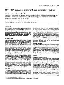
(a) An RNA Secondary Structure

(b) Its corresponding tree representation

Figure 1: Tree representation for RNA secondary structure Traditionally, when an RNA structure has either dangling heads or tails, the structure is represented as a forest instead of a tree. So, in order to overcome this limitation, a virtual root may be used to combine the

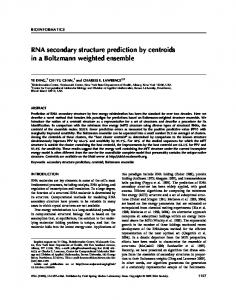
forest trees in one single tree. For example, Figure 1(b) illustrates this idea for mapping of the RNA structure shown in Figure 1(a) to a forest consisting of three trees shown under the virtual root called “RNA”. However, combining the forest trees in one big tree still suffers from an interesting problem. In an ordered tree, the relative order of the ancestor and sibling nodes is significant. Consequently, any tree-alignment solution should respect this property by matching siblings to siblings and ancestors to ancestors. Unfortunately, this constraint would make some alignments impossible for some trees represented like Figure 1(b). For example, consider the two RNA molecules shown Figure 2(a) and their traditional tree representations shown in Figure 2(b). From a biological perspective, the dangling tail “A” in RNA-1 should be mapped to the base “A” of pair “U-A” in RNA-2 while the two “G-C” base pairs should be mapped to each other. However, the above relativeorder preservation constraint makes this mapping impossible: i.e. for the two base-pair “G-C”, it is impossible to partially match the base “A” (which is a sibling) to the pair “U-A” which is a parent.

RNA-1 RNA-2

(a) Two RNA structures

3. The SRPC algorithm Representing the RNA structure as an ordered labeled tree as discussed in the last section, the problem of RNA structure comparison becomes a problem of "ordered labeled-tree comparison", to which the ZhangShasha tree-editing algorithm 18 can be applied. The Zhang-Shasha algorithm is concerned about calculating the minimum editing distance between the given trees regardless of the associated editing operations. In this work, we have implemented SPRC, an extension of the Zhang-Shasha algorithm, to actually record the operations’ sequence that lead to each calculated sub-tree distance in a configuration matrix, called candidacy matrix. The actual edit-operation sequence corresponding to a particular edit distance can be found by following the path segments stored in the candidacy matrix, from its lower right up to its upper left corner. In general, there is more than one solution (editoperation sequence) for any given minimum edit cost. In the context of the RNA structure-comparison problem, each of these edit-operation sequences corresponds to a different sequence of evolutionary operations that may have led to the production of one molecule from the other. Clearly, not all such evolutionary paths are equally likely. This is why, in SPRC, we have developed (a) an affine biologically inspired cost function to guide the tree-alignment process, and (b) a set of heuristic filters designed to select the most likely solution of the ones with the same minimum cost based on the overall “Occam’s Razor” intuition that “simpler” sequences are more likely.

3.1

RNA-1 RNA-2

RNA-1 RNA-2

(b) Traditional tree representation

(c) SPRC’s representation

Figure 2: Representation of Dangling heading/tails To overcome this problem, we have developed a variant fine-grained tree representation where a dangling base is represented as a node that is the parent of other dangling bases or base pairs. For example, Figure 2(c) illustrates that dangling base "U" is represented as "_U" which is the parent of the dangling node "_A" which (in order) is the parent of the very first base pair of the structure. It is clear that applying the same representation on the example of Figure 2 would make the target biological alignment possible.

Cost Function

Based on SPRC’s representation for RNA, we have adopted a cost function conforming to the following biologically motivated intuitions: • Deleting (or inserting) a base pair should be more expensive than deleting a single base. Thus, the cost of deleting (or inserting) a single base is 2 and the corresponding cost for a base pair is 10. • Deleting a dangling base should be relatively easier than deleting a single base in the loop region (cost = 1); • Deleting the opening base pair of a hairpin loop should be slightly easier than deleting the other base pairs, since it does not create a local secondary structure unit change (cost = 9). • Mutating a nucleotide of either a single base or a base pair to another nucleotide should be cheaper than deletion (cost = 1). Consequently, mutating both nucleotides in a base pair is assigned a cost of 2.

• Mapping a dangling base to a base pair is assigned a cost equivalent to the sum of costs involved in (a) matching the dangling base to the corresponding nucleotide in that pair, plus (b) the cost of breaking this pair. The cost of breaking a base pair varies according to the depth of the pair in the structure, counted from the beginning of the secondary structure. The cost of breaking a base pair is equal to the depth of the base pair in the tree. • All other mutations are assigned the cost of deleting the first member plus the cost of inserting the second one. The SPRC algorithm applies the above cost function using an affine-based scheme. tdist (T1[l (i )..i ], T2 [l ( j ).. j ])    fdist (T1[l (i )..i − 1], T2 [l ( j ).. j − 1]) + γ (i, j )  (i,−) eligibledelete (i, j , l (i )) γ = min  fdist (T1[l (i )..i − 1], T2 [l ( j ).. j ]) +  affine γ ( i , −) otherwise    γ affine (−, j ) eligibleinsert (i, j , l ( j ))  fdist (T1[l (i )..i ], T2 [l ( j ).. j − 1]) +  otherwise  γ (−, j ) 

discussed in the subsequent sections were conceived to minimize the cardinality of the original solution set to a small subset – ideally of cardinality 1 – that includes the more biologically likely solutions.

4. Defining Simplicity The objective of SPRC’s simplicity filter is to discard the biologically unlikely solutions from the solution set produced by the SPRC tree-alignment algorithm.

4.1

Path Minimality

The first simplicity heuristic advises the algorithm to “prefer minimal paths”: when there is more than one different path with the same minimum cost, the one with the least number of deletion and/or insertion operations is preferable.

fdist (T1[l (i1 )..i ], T2 [l ( j1 ).. j ])    fdist (T1[l (i1 )..l (i ) − 1], T2 [l ( j1 )..l ( j ) − 1]) + tdist (T1[l (i )..i ], T2 [l ( j ).. j ])  (i,−) eligibledelete (i, j , l (i )) γ = min  fdist (T1[l (i1 )..i − 1], T2 [l ( j1 ).. j ]) +  affine otherwise  γ (i,−)   γ affine (−, j ) eligibleinsert (i, j , l ( j ))  fdist (T1[l (i1 )..i ], T2 [l ( j1 ).. j − 1]) +  otherwise   γ (−, j )

where l (i ) is the leftmost child of i, and function

γ is the cost

eligibledelete (i, j , left ) true i = left & delete ∈ c(i, j )  = eligibledelete (i − 1, j , left ) i > left & delete ∈ c(i, j )

The idea of affine cost was originally introduced in the context of sequence alignment. The underlying intuition is that insertions and deletions often occur in multiples, when the same mutation operator has affected a sequence of neighboring nucleotides. In such cases, the cost of this set of mutations should be less than the sum of the same number of individual mutations. SPRC implements the affine-cost policy by assigning contiguous deletions/insertions the cost of opening a gap plus a constant factor times the number of deleted/inserted nodes. This policy is implemented using the candidacy matrix (discussed in the previous section), which records the possible edit operation(s) associated with each tree node (i.e., RNA base). The candidacy matrix is consulted about whether all the children of a given node are candidates for deletion/insertion; if so, then an affine-cost policy applies to this node instead of the regular cost policy. In general, our algorithm equipped with the cost function described in this section, results in a set of possible edit-operation sequences, all with the same minimum edit cost. The three filtering heuristics

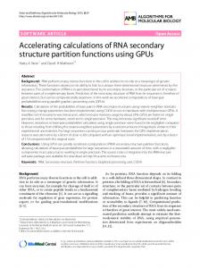
(a) P1

(a) P2

Figure 3: Minimizing the number of edit operations For example, consider the trees T1 and T2 shown in Figure 3(a). Using the scoring scheme explained in section 3.1, there are two possible editing paths with the same minimum cost: p1 shown in Figure 3(a) and p2 shown in Figure 3(b), where the cost of deleting a base pair T1[10]="AU" is equivalent to the cost of deleting all the single bases T2[1…5]={"U", “G”, "C", "G", "A"}. Similarly, the cost of inserting a base pair T2[10]="AU" equals the total cost of inserting the single bases T1[1…5]={"U", “G”, "C", "G", "A"}. While both p1 and p2 have the same global editing cost, each of them represents a different edit path. According to the path-minimality heuristic, p1 should be preferred because it contains the smaller set of edit operations. From a biological perspective, this heuristic captures the intuition that a smaller set of mutation operations is, in principle, more likely than a larger one.

4.2

Vertical Refraction Points

The second simplicity heuristic advises the algorithm to “prefer contiguous similar edit operations”. Intuitively, this rule says that the contiguous same edit operations could be one single operation that involves long segments of nucleotides, and thus is more biologically likely. When there are multiple different paths with the same minimum cost and the same

number of editing operations, the one with the least number of changes (refractions) of operation types along a tree branch is preferable. This heuristic also makes sense from a biology point of view: it is more likely that similar mutations will happen in contiguous bases (either pairs or singles) rather than in dispersed ones. In other words, for an RNA sub-structure's member, it is more likely to have the same kind of mutation as the opening pair, than to have a different kind of mutation.

operation applied to its parent differs from the operation applied to this node. For example, solution p1 shown in Figure 4(b) has 6 refraction points that are visualized as dashed connectors to their parents; contrast this with either p2 or p3 that each has 2 refraction points only. Hence, p2 and p3 simpler than p1 as they have less number of vertical refraction points. We have to note that vertical simplicity is similar to the affine-cost policy except that the affine policy is applied local to a certain node with its children, while the vertical simplicity is globally applied to a whole tree. In other words, the affine-cost policy is used while developing the solution set to promote subsolutions that may be impossible without an affinecost; however, vertical simplicity is used as a postprocessing filtration step to choose the biological best global solutions out of the developed ones.

4.3

(a) Two RNA structures

(b) Solution P1

Horizontal Refraction Points

In addition to maximizing the number of nodes along a tree branch to which the same edit operation is applied, SPRC also proposes that, to the extent possible, sibling nodes should also suffer the same edit operations. According to this third heuristic, solution p3 is preferable to p2 since it applies deletion operations to all members (T1[1] and T1[7]) of the bulge loop opened by T1[8], while in p2, T1[7] is to be relabeled and T1[1] is to be deleted. From a biological perspective, this filtering heuristic considers the interior of a loop's body (e.g. internal, bulge, and hairpin loops) and prefers solutions that have similar editing operations on contiguous sibling nodes.

(c) Solution P2

(d) Solution P3

Figure 4: Alternative Editing Paths with different numbers of Refraction Points Consider, for example, the three different edit paths shown in Figure 4: both p2 and p3 are simpler than p1 since in both of them all deletion operations are applied to a contiguous sequence of nodes along the tree branch. More specifically, in p1 shown in Figure 4(b) and especially in the stack loop T1[9..10], the mutation that happens at the opening base pair T1[10] (which is to be deleted) differs from the mutation that happens at the closing pair, T1[9] (which is to be relabeled). Similarly for the stack loop T1[8..9], the mutation happens for the opening pair differs from the one happens at the closing one. Neither p2, nor p3 contain such an implausible set of mutations, and that makes them preferable to p1 according to this heuristic. This heuristic is implemented by counting the number of vertical refraction points. A vertical refraction point is defined as a node where the editing

Sibling simplicity is measured by the number of horizontal refraction points. A horizontal refraction point is defined as a node where the applied operation to its sibling differs from the operation applied to this node. For example, p2 and p3 have 1 and 0 horizontal refraction points respectively; in p2, the operation applied to T1[1] (which is to be deleted) differs from the operation applied to its sibling T1[7] (which is to be changed/relabeled) while in p3 there are no sibling refraction points. Hence, solution p3 is selected as the simplest editing solution for the two compared trees.

5. Evaluation This section evaluates our implementation of the SPRC method in two ways: first, we evaluate SPRC’s phase 1, i.e., our extension of the Zhang-Shasha algorithm, based on both the proposed tree representation and cost function; second, we evaluate the effectiveness of SPRC’s phase 2, i.e., the application of the simplicity heuristics as a filtration step.

All the evaluations shown in this section has been measured based on experiments done on three 5S ribosomal families: archeaa (3,825 problems), eubacteria (156,919 problems), and eukaryota (51,410 problems). 5S ribosomal RNA is an integral component of the large subunit of all cytoplasmic and most organeller ribosomes. Its small size and association with ribosomal as well as non-ribosomal proteins made it an ideal model RNA molecule for studies of RNA structure and RNA-protein interactions. The multiple sequence alignments of 5S ribosomal RNAs are provided where base pairs in phylogenetically conserved secondary structures are specified 16. For each pair of RNA secondary molecules within a family, we first applied the SRPC structurecomparison algorithm, to calculate the minimum-cost edit distance and to record the minimum-cost edit sequences. For many cases – 79.74%, 73.99%, and 43.49% for each of the three families, respectively – multiple minimum-cost alignments were found; we call the generated set of alignments the solution set. For each pair, the target solution, i.e., the correct alignment is published at the 5S Ribosomal RNA database [5S]. Therefore, we can assess the quality of each solution set by comparing it against the published target solution. For that purpose, we designed a metric, called percent of disagreement (POD), to measure how far a given alignment is from the target one. The POD of an alignment is calculated as the number of bases in the two compared structures that are aligned differently in the target alignment, divided by the sum of both lengths; when POD equals zero, the two alignments are identical. In order to evaluate the quality of a solution set, we compute both the minimum and maximum PODs; the minimum POD refers to the closest (best) solution to the target one, while the maximum POD refers to the farthest (worst) solution within that set. Finally, for each pair we obtained the alignment proposed by the RNA-Align tool [19] as a baseline representative of the state-of theart tools in RNA alignment.

5 . 1 Tree representation function

and

Cost

Table 1 shows the quality evaluation of the results from SPRC’s phase 1 against the results from RNA Align 3[19]. Table 1 shows that for the three families: Archeaa, Eubacteria, and Eukaryota, the target solutions are included in the SPRC solution sets with percentages 27.35%, 40.80%, and 82.52%, respectively. In contrast, RNA Align produced the target solution for only 11.74%, 19.56%, and 70.97%, of the cases respectively.

Additionally, Table 1 shows a general comparison between the results of SPRC and RNA Align; it shows the percentages of the cases where: • RNA Align results are better than SPRC, i.e., the POD of RNA Align is less than the minimum (best) POD in SPRC’s solution set. • Both results are equal, i.e., the POD of RNA Align is within the max and min PODs of SPRC’s solution set. • SPRC is better, i.e., the POD of RNA Align is greater than the maximum (worst) POD in SPRC’s solution set. An interesting result is that for Archeaa family, SPRC is 2.3 times better than RNA Align in including the target solution in the produced solution sets. Another interesting result is that for the Archeaa family, the quality of SPRC’s results is twice as good as those of RNA Align. Generally, the SPRC is better than RNA Align in including the target solution in the produced solution sets: with 50.67% compared to 31.88% for RNA Align. Additionally, the quality of the results produced by SPRC’s phase 1 is better than those of RNA Align: with 21.64% for SPRC compared to 18.57% for RNA Align. Therefore, it is clear that in general, SPRC is better than RNA Align. Hence, the used tree representation and cost function are reliable. Table 1: Comparison to RNA Align POD = 0 (Target solution General Quality Family No. of is produced) Name Problems RNA SPRC’s RNA Both are SPRC Align Phase 1 Align is comparable is better better Archeaa 3,825 11.74% 27.35% 16.63% 48.50% 34.87% Eubacteria 156,919 19.56% 40.80% 23.56% 48.82% 27.62% Eukaryota 51,410 70.97% 82.52% 3.5% 94.1% 2.4% Total 212,154 31.88% 50.67% 18.57% 59.79% 21.64%

5.2

Simplification feasibility

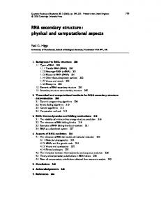
Figure 5 shows how the cardinalities (sizes) of solution sets were reduced by the filtration process for each of the Archeaa family. It shows that the number of problems with high cardinalities was reduced while the number of problems with low cardinality was increased. This figure shows histogram of problems for which the cardinalities of the solution sets produced by the SRPC algorithm and filtered through the three SRPC heuristics were 1, 2, …, 9 and more than 9. The last category is especially interesting: for example, there were 1489 problems for which SPRC’s phase 1 produced a set of more than 9 solutions – the corresponding number after the heuristics were applied was 242. Consider for example the largest solution set produced by the SRPC algorithm, which was the

comparison of “Desulfurococcus mobilis 1” versus “Methanothermobacter thermautotrophicus 5”: the original solution set included 13,230 possible alignments while the corresponding number after the heuristics were applied was 12. Based on this data, it is clear that the filtering heuristics are very effective in minimizing the cardinality of possible alignments and thus focusing the attention of RNA researchers on a smaller set of alignments.

solution with 99.55%, 83.97%, and 88.52%, respectively; while managed to reduce the average number of solutions from 59.28 to 58.62, 9.69, and 3.25 respectively. As a measure of the general quality of the whole process, we computed the percentage of problems for which the best solution was included in the final solution set resulting from the three filtering steps. This number, for each of the three families Archeaa, Eubactria, and Eukaryota, was 76.65%, 89.95%, and 95.98%, respectively. The results reported in the last row of the Table show that, in general, SPRC’s filtration process is capable of reducing (in average) the solution set size from 12.24 to 2.33 with general quality 90.55% of keeping the best given solution in the filtered set. Table 2: Simplification Quality

Figure 5: The impact of the Simplicity Heuristics in the Archeaa Family

Simplicity Heuristics Size of Shortest Vertically Horizontal Avg. Family Problem path Simplest Simplest Card. Set Avg. Quality Avg. Quality Avg. Quality Card. (%) Card. (%) Card. (%) Archeaa 3,825 59.28 58.62 99.55 9.69 83.97 3.25 88.52 Eubactria 156,919 14.5 14.34 99.9 5.1 95.8 2.58 92.57 Eukaryota 51,410 1.88 1.87 1 0 0 1.81 99.87 1.5 96.04 Total 212,154 12.24 12.11 99.91% 4.38 96.57 2.33 93.33

6. Conclusions The question then becomes “how effective are the heuristics in actually selecting the most biologically likely alignment”? In order to answer this question, for each solution set, we calculated the minimum PODs both before and after the heuristics are applied, and then if both PODs are the same, then the heuristics managed to keep the best given solution in the simplified set, otherwise, it failed. Table 2 shows the results of applying the above quality measure for each of the three simplicity heuristics. For each family, Table 2 shows: • Number of problems in the experiment • Average cardinality of the original solution set, i.e., the average number of solutions contained in the sets produced by SPRC’s phase 1. • For each of the three filtration steps, i.e., shortest path, vertical simplicity, and horizontal simplicity: o the average cardinality upon the completion of the step given the cardinality of the previous step. o The quality of the step, which is calculated by comparing the minimum POD of filtered the solution set to the minimum POD of the same set just before applying this filtration step; if both POD are same then the filtration is good because it kept the best solution in the filtered set. For example, it shows that for Archeaa, the three heuristics: “Shortest path”, “Vertically Simplest”, and “Horizontal Simplest” managed to keep the best given

The correctness of RNA-comparison methods depends on the precision of the biological information modeled in the data representation, and the method’s scheme for assessing the cost of different kinds of mutations, inversely related to their probability of occurrence. In this paper, we discuss our SPRC method, for RNA structure comparison. In our work, we developed, a novel tree representation of RNA that reflects both its primary and secondary structure and a tree-alignment algorithm, which, given the tree representations of two RNA molecules, produces a sequence of mutations that could transform one RNA molecule to the other. Our SPRC algorithm extends the Zhang-Shasha tree-edit distance calculation algorithm in two ways: first, in addition to the distance, it reports all editing sequences with the same minimum edit cost, and second, it uses a biologicallyinspired affine cost function. Furthermore, the SPRC method proposes set of heuristics designed to filter the produced solution set to recommend the simplest editing sequence, as corresponding to the most biologically correct alignment. Our experiments show that SPRC is capable with percentage 50.67% to produce the exact target solution compared to 31.88% of related work like RNA Align. Clearly, there is still plenty of room for improvement. However, it is important to note that the average POD

of the solution sets is 2.22%: this implies that even when the exact solution is not included in the SPRC solution set, the included solutions are very close to the correct one, i.e., there is a very small ratio of disagreement between them. Based on this evidence, we can argue that the SRPC tree representation and scoring scheme are biologically meaningful and therefore potentially useful for biologists inspecting its results. Furthermore, our experiments show that the simplicity heuristics are very effective in reducing the cardinality of solution sets while keeping the qualified solutions; on average, the cardinality was reduced 5.25 times while keeping the best solution in the solution set, in 90.55% of the cases. This evidence supports our hypothesis that the SRPC simplicity heuristics are indeed biologically meaningful. In the future, we plan to work on improving the cost function and on extending the tree representation to better reflect the secondary RNA structure.

References 1.

S. Altschul, W. Gish , W. Miller, E. Myers, and D. Lipman. "Basic local alignment search tool." Journal of Molecular Biology, 215 (1990): 403--410.

2.

S. Altschul, T. Madden, A. Schaffer, J. Zhang, Z. Zhang, W. Miller, D. Lipman. “Gapped BLAST and PSI-BLAST: a new generation of protein database search programs.” Nucleic Acids Research, 25 (1997): 3389--3402.

3.

G. Collins, S. Le, and K. Zhang. "A new algorithm for computing similarity between RNA structures." Information Sciences 139, issue 1-2(2001): 59--77.

4.

5.

S. Dulucq, and Laurent Tichit. “RNA Secondary structure comparison: exact analysis of the Zhang–Shasha tree edit algorithm.” Theoretical Computer Science, 306, issue 1-3(2003): 471--484. M. Hoechsmann, T. Toeller, R. Giegerich, S. Kurtz. “Local Similarity of RNA Secondary Structures.” Proceedings of Computational Systems Bioinformatics (2003): 159--168.

6.

I. Hofacker, W. Fontana, P. Stadler, L. S. Bonhoeffer, M. Tacker, and P. Schuster. “Fast Folding and Comparison of RNA Secondary Structures.” Chemical Monthly 125, issue 2(1994): 167--188.

7.

L. Wang and D. Gusfield. “Improved approximation algorithms for tree alignment.” Proceedings of the 7th Combinatorial Pattern Matching conference (1996) 220--233.

8.

C. Isert. “The Editing Distance Between Trees.” http://citeseer.ist.psu.edu/isert99editing.html (accessed Aug. 2006)

9.

T. Jiang, L. Wang, and K. Zhang. “Alignment for trees -an alternative to tree edit.” Proceedings of the 5th

Annual Symposium on Combinatorial Pattern Matching, Lecture Notes In Computer Science, 807 (1994): 75--86. 10. S. Le, R. Nussinov, and J. Mazel. “Tree graphs of RNA secondary structures and their comparison.” Computational Biomedical Research, 22 (1989): 461--473. 11. B. Ma, L. Wang, and K. Zhang. “Computing similarity between RNA structures.” Theoretical Computer Science, 276 (2002): 111--132. 12. T. Munzner, F. Guimbretiere, S. Tasiran, L. Zhang, and Y. Zhou. “TreeJuxtaposer: Scalable Tree Comparison using Focus+Context with Guaranteed Visibility.” SIGGRAPH, published as ACM Transactions o n Graphics 22, issue 3 (2003): 453--462. 1 3 . D. Sankoff and R. Cedergren. “Simultaneous comparison of tree or more sequences related by a tree.” In D. Sankoff and G. Kruskal, editors, Time Warps, String Edits, and Marcomolecules: the Theory and Practice of Sequence Comparison, 2 8 (1983): 253--263. 14. S. M. Selkow. “The tree-to-tree editing problem.” Information Processing Letters, 6 (1977): 184--86. 15. B. Shapiro. “An algorithm for comparing multiple RNA secondary stuctures.” Comp. Appl. Biosci. 4, issue 3(1988): 387--393. 16. M. Szymanski, M. Barciszewska, V. Erdmann, and J. Barciszewski. “5S ribosomal RNA database” Nucleic Acids Res. 30: 176--178. 1 7 . K. Tai. “The Tree-to-tree Correction Problem”. Journal of ACM 26 (1979), 422--433. 18. K. Zhang, R. Stgatman, and D. Shasha. “Simple fast algorithm for the editing distance between trees and related problems.” SIAM Journal on Computing, 18(6): 1245--1262. 1

9T h. e RNA match package: http://www.csd.uwo.ca/~kzhang/rna/rna_match.html (accessed Aug. 2006)

2 0 .RNAForester Online: http://bibiserv.techfak.unibielefeld.de/rnaforester/ (accessed Aug. 2006)