Dec 5, 2014 - subclasses of decoding rules: The first is a function of the output vector only, ... Erasure/list decoding, mismatch decoding, random coding, error ...
1
Simplified Erasure/List Decoding Nir Weinberger and Neri Merhav Dept. of Electrical Engineering Technion - Israel Institute of Technology Technion City, Haifa 3200004, Israel
arXiv:1412.1964v1 [cs.IT] 5 Dec 2014
{nirwein@tx, merhav@ee}.technion.ac.il
Abstract We consider the problem of erasure/list decoding using certain classes of simplified decoders. Specifically, we assume a class of erasure/list decoders, such that a codeword is in the list if its likelihood is larger than a threshold. This class of decoders both approximates the optimal decoder of Forney, and also includes the following simplified subclasses of decoding rules: The first is a function of the output vector only, but not the codebook (which is most suitable for high rates), and the second is a scaled version of the maximum likelihood decoder (which is most suitable for low rates). We provide single-letter expressions for the exact random coding exponents of any decoder in these classes, operating over a discrete memoryless channel. For each class of decoders, we find the optimal decoder within the class, in the sense that it maximizes the erasure/list exponent, under a given constraint on the error exponent. We establish the optimality of the simplified decoders of the first and second kind for low and high rates, respectively. Index Terms Erasure/list decoding, mismatch decoding, random coding, error exponents, decoding complexity.
I. I NTRODUCTION An ordinary decoder must always decide on a single codeword, and consequently, its decision regions form a partition of the space of output vectors. In his seminal paper [1], Forney defined a family of generalized decoders with decision regions which do not necessarily satisfy the above property. An erasure decoder has the freedom not to decode, and so, its decision regions are disjoint but not necessarily cover of the space of channel output vectors. A list decoder may decide on more than one codeword, thus its decision regions may overlap. An erasure/list decoder can practically be used in cases where an additional mechanism is used to resolve the ambiguity left after a nondecisive decoding instance. For example, if the transmitted codewords at different times are somewhat dependent, then an outer decoder may recover from an erasure by “interpolating” from neighboring codewords, or eliminate all codewords in the list, but one. Such a case is present in concatenated codes where the inner decoder may be an erasure/list decoder. As another example, consider the case where a feedback link may signal the transmitter on an erasure event. In this case, the transmitter may send repeatedly the codeword until there is no erasure. Indeed, this
2
is the case in rateless codes [2], [3], where at each time instant, the decoder needs to decide whether to continue acquiring additional output symbols, or decide on the transmitted codeword. When considering list decoders, a distinction should be made between list decoders with a fixed list size (see for example [4], and references therein), and decoders for which the list size is a function of the output vector and thus a random variable. In the latter case, a natural trade-off in designing the decoder is the error probability, i.e., the probability that the correct codeword is not on the list, and the average list size. In [1], Forney has generalized the Neyman-Pearson Lemma and derived the decoder which optimally trades off between error probability and average list-size. This optimal list decoder and the optimal erasure decoder (which optimally trades off between error probability and erasure probability), were found to have the same structure. In addition, Forney has extended the analysis of Gallager for ordinary decoding [5, Chapter 5], and derived lower bounds on the random coding error exponent and the list size exponent (the normalized logarithm of the expected list size). More recently, Somekh-Baruch and Merhav [6] have found exact expressions for the random coding exponents, inspired by the statistical-mechanics perspective on ensembles of random codes [7]. Over the years, research was aimed towards various extensions. For example, in [8, Chapter 10] [9], [10], [11] universal versions of erasure/list decoders, i.e., decoders that perform well even under channel uncertainty. In [12], the size of the list was gauged by its ρ-th moment, where ρ = 1 corresponds to the average list size, as in [1], and an achievable pair of error exponent and list size exponents was found. In essence, as we shall see, Forney’s optimal erasure/list decoder is conceptually simple - a codeword belongs to the output list if its a posteriori probability, conditioned on the output vector, is larger than a fixed threshold. However, as is well known, the prospective implementation of such a decoder is notoriously difficult, since it requires the calculation of the sum of likelihoods (c.f. Subsection II-B). These likelihoods typically decrease exponentially as the block length increases, and thus have a large dynamic range. Therefore, an exact computation of this sum is usually not feasible. Moreover, the number of summands is equal to the number of codewords and thus increases exponentially with the block length. In fact, it was proposed already by Forney himself to approximate this sum by its maximal element [1, eq. (11a)]. It is the purpose of this paper to study classes of simplified decoders which avoid the need to confront such numerical difficulties. To this end, we first formulate the optimal erasure/list decoder as a threshold decoder, and propose to replace the optimal threshold with a threshold from a fairly general class. Any threshold from this class may represent some complexity constraint of the decoder. We then consider two subclasses of this class of decoders. For the first subclass, which is well suited for high rates, the threshold function is extremely simple it depends on the output vector only. For the second subclass, which is well suited for low rates, the threshold is the log-likelihood (plus an additive fixed term), which is the approximation proposed by Forney. Then, for a given discrete memoryless channel (DMC), we derive the exact random coding exponents for the ensemble of fixed composition codebooks, associated with decoders from the above general class and its two subclasses. Next, for the general class of decoders, and for its two subclasses, we find the optimum decoder, within the given class,
3
which achieves the largest list size exponent for a prescribed error exponent. This enables the establishment of the optimality of the simplified decoders of the first and second kind, for low and high rates, respectively. The outline of the rest of the paper is as follows. In Section II, we establish notation conventions, provide some background of known results, and define the relevant classes of decoders. In Section III, we derive the exact random coding exponents for all defined decoders, and in Section IV, we find the optimal decoder within each class. In Section V, we discuss the optimality of the various simplified decoders defined, for low and high rates. Finally, in Section VI, we compare the random coding exponents of the optimal decoder, as obtained in [6], with the exponents of the suboptimal decoders, for simple numerical examples. All the proofs are deferred to Appendix A. II. P ROBLEM F ORMULATION A. Notation Conventions Throughout the paper, random variables will be denoted by capital letters, specific values they may take will be denoted by the corresponding lower case letters, and their alphabets, similarly as other sets, will be denoted by calligraphic letters. Random vectors and their realizations will be denoted, respectively, by capital letters and the corresponding lower case letters, both in the bold face font. Their alphabets will be superscripted by their dimensions. For example, the random vector X = (X1 , . . . , Xn ), (n - positive integer) may take a specific vector value x = (x1 , . . . , xn ) in X n , the n-th order Cartesian power of X , which is the alphabet of each component of this vector. A joint distribution of a pair of random variables (X, Y ) on X × Y , the Cartesian product alphabet of X and Y , ˜ XY . Usually, we will abbreviate this notation by omitting the will be denoted by QXY and similar forms, e.g. Q
subscript XY , and denote, e.g, QXY by Q. The X -marginal (Y -marginal), induced by Q will be denoted by QX (respectively, QY ), and the conditional distributions will be denoted by QY |X and QX|Y . In accordance with this notation, the joint distribution induced by QX and QY |X will be denoted by QX × QY |X , i.e. Q = QX × QY |X . ˆ x denote the empirical distribution, that is, the vector {Q ˆ x (x), x ∈ X }, where Q ˆ x (x) For a given vector x, let Q
is the relative frequency of the letter x in the vector x. Let TP denote the type class associated with P , that is, the ˆ x = P . Similarly, for a pair of vectors (x, y), the empirical joint distribution set of all sequences {x} for which Q ˆ xy . will be denoted by Q
The mutual information of a joint distribution Q will be denoted by I(Q), where Q may also be an empirical joint distribution. The information divergence between Q and P will be denoted by D(QkP ), and the conditional information divergence between the empirical conditional distribution QY |X and PY |X , averaged over QX , will be denoted by D(QY |X kPY |X |QX ). Here too, the distributions may be empirical. The probability of an event A will be denoted by P{A}, and the expectation operator will be denoted by E{·}. Whenever there is room for ambiguity, the underlying probability distribution Q will appear as a subscript, e.g., EQ {·}. The indicator function will be denoted by I{·}. Sets will normally be denoted by calligraphic letters. The probability simplex over an alphabet X will be denoted by S(X ). The complement of a set A will be denoted by
4
A. Logarithms and exponents will be understood to be taken to the natural base. The notation [t]+ will stand for . max{t, 0}. For two positive sequences, {an } and {bn }, the notation an = bn will mean asymptotic equivalence in
the exponential scale, that is, limn→∞
1 n
log( abnn ) = 0.
B. System Model and Background Consider a DMC, characterized by a finite input alphabet X , a finite output alphabet Y , and a given matrix of single-letter transition probabilities {W (y|x), x ∈ X , y ∈ Y}. Conditioning on the channel input X = x, the distribution of the output Y is given by P(Y =y|X = x) =
n Y
W (yi |xi ).
(1)
i=1
We will use the shorthand notations P (x, y) , P(X = x, Y = y), P (y|x) , P(Y = y|X = x), and P (x|y) , P(X = x|Y = y). Let R be the coding rate in nats per channel use, and let C = {x1 , x2 . . . , xM }, xm ∈ X n , m = 1, . . . , M , M = enR denote the codebook.
An erasure/list decoder φ is a mapping from the space of output vectors Y n to the set of subsets of {1, . . . , M } (i.e., φ : Y n → P({1, . . . , M }), where the latter is the power set of {1, . . . , M }). Alternatively, an erasure/list n decoder φ is uniquely defined by a set of M + 1 decoding regions {Rm }M m=0 such that Rm ⊆ Y and R0 = S Y n\ M m=1 Rm . Given an output vector y, the mth codeword belongs to the list if y ∈ Rm , and if y ∈ R0 an
erasure is declared.
The average error probability of a list decoder φ and a codebook C is the probability that the actual transmitted codeword does not belong to the list, Pe (C, φ) ,
M 1 X X P (y|xm ). M
(2)
m=1 y∈Rm
The average number of erroneous codewords on the list is defined as L(C, φ) ,
M X 1 X X P (y|xm ) I(y ∈ Rl ) M n
(3)
1 M
(4)
m=1
y∈Y
=
M X
X X
l6=m
P (y|xm ).
l=1 y∈Rl m6=l
If the decoder never outputs more than one codeword, then it is termed a pure erasure decoder. In this case, Pe (C, φ) designates the total error probability (which is the sum of the erasure probability and undetected error probability), and L(C, φ) designates the undetected error probability. In what follows, we shall describe our results with the more general erasure/list terms, but unless otherwise stated, the results are also valid for pure erasure decoders, with the above interpretation. In [1], Forney has generalized the Neyman-Pearson lemma, and obtained a class of decoders Φ∗ , {φT , T ∈ IR} which achieves the optimal trade-off between Pe (C, φ) and L(C, φ). The decoding regions for a decoder φT ∈ Φ∗
5
are given by R∗m
,
(
)
P (y|xm ) y: P ≥ enT P (y|x ) l l6=m
, 1 ≤ m ≤ M.
(5)
The parameter T is called the threshold, and it controls the trade-off between Pe (C, φ) and L(C, φ). As T increases, the list size typically becomes smaller, but in exchange, the error probability increases. To obtain a pure erasure decoder, the threshold T should be chosen non-negative. For T < 0, an erasure/list decoder is obtained. As a figure of merit for a decoder, we will consider its random coding exponents, over the ensemble of fixed composition codes with input distribution PX . For this ensemble, the M = enR codewords of C = {x1 , . . . , xM } are selected independently at random under the uniform distribution across the type class TPX . We denote the averaging over this ensemble of random codebooks by overlines. The random coding error exponent is defined as 1 Ee (R, φ) , lim inf − log Pe (C, φ) n→∞ n
(6)
and the random coding list size (negative) exponent is defined as 1 El (R, φ) , lim inf − log L(C, φ). n→∞ n
(7)
Notice that Ee (R, φ) ≥ 0 but El (R, φ) may also be negative, which means that the random coding list size may increase exponentially. In [6], the exact random coding exponents for a decoder φ∗T ∈ Φ∗ , which we denote by Ee∗ (R, T ) and El∗ (R, T ), were found1 . Defining Ea (R, T ) , min
min
˜ Q: QY =Q ˜ Y ,f (Q)+T ≥f (Q),I(Q)≥R ˜ Q
n
o ˜ Y |X ||W |PX ) + I(Q) − R, D(Q
(8)
and ˜ Y |X ||W |PX ), Eb (R, T ) , min D(Q
(9)
˜ Q∈L
where L,
(
˜ : f (Q) ˜ ≤R+T + Q
max
˜ Y ,I(Q)≤R Q: QY =Q
)
[f (Q) − I(Q)] ,
(10)
we have that Ee∗ (R, T ) = min{Ea (R, T ), Eb (R, T )}
(11)
El∗ (R, T ) = Ee∗ (R, T ) + T.
(12)
and [11, Lemma 1]
In the rest of the paper, we will consider simplified erasure/list decoding which determine if a codeword belongs to the list, by checking if the likelihood of the codeword is larger than some threshold function. To motivate 1
See Appendix B for a justification of the applicability of the results in [6] also for the case T < 0.
6
this approach, we first inspect the optimal decoder (5) in more detail. In its current form, the optimal decoder P is essentially infeasible to implement. The reason for this is that the computation of l6=m P (y|xl ) is usually
intractable, as it is a sum of exponentially many likelihood terms, where each likelihood term is also exponentially small. This is in sharp contrast to ordinary decoders, based on comparison of single likelihood terms which can be carried out in the logarithmic scale, rendering them numerically feasible. However, the optimal decoder can be simplified without asymptotic loss in exponents. To see this, we need first some notation: for a given joint type Q and output vector y, let Nm (Q|y) be the number of codewords other than xm in C , whose joint empirical
distribution with y is Q. Now, define the decision regions � � ˆ xm y ) nf (Q nT nf (Q) ˜ Rm , y : e ≥ e max Nm (Q|y) · e , 1 ≤ m ≤ M, Q
(13)
where f (Q) is the normalized log-likelihood ratio, namely f (Q) ,
X
Q(x, y) log W (y|x).
(14)
x∈X ,y∈Y
We have the following observation. ˜ m }M are the same Proposition 1. The random coding error- and list size exponents of the decoder defined by {R m=1
as the random coding error- and list size exponents of the optimal decoder (defined by {R∗m }M m=1 ). We will refer to the right-hand side of (13) as the threshold of the decoder. The focus of this paper, is the performance of erasure/list decoders for which the threshold function is not necessarily the optimal threshold dictated by (13). The motivation for such an erasure/list decoder is that the threshold function employed may be simpler to compute. Observe, that the threshold of (13) only depends on the joint type of each competing codeword (l 6= m) with the output vector. Therefore, we propose to consider the class of decoders Ψ , {φh , h : S(X × Y) → IR}, defined by a continuous function h(·) in some compact domain G ⊆ S(X × Y), and infinite elsewhere2. The decoding regions of φh ∈ Ψ are given by o n ˆ ˆ Rm = y : enf (Qxm y ) ≥ en·maxl6=m h(Qxl y ) , 1 ≤ m ≤ M. As discussed above, for this decoding rule, computations may be carried in the logarithmic domain as � � ˆ ˆ Rm = y : f (Qxm y ) ≥ max h(Qxl y ) . l6=m
(15)
(16)
With a slight abuse of notation, we shall denote the random coding exponents of φh ∈ Ψ by Ee (R, h) and El (R, h). Note that in (15), the threshold function is assumed to be the same for all codebooks in the ensemble (for specific rate R). In contrast, for the asymptotically optimal decoder (13), the threshold is tuned to the specific codebook employed. This modification reduces complexity (though only slightly) and may, in general, degrade the exponents. 2
The set G will be a strict subset of S(X × Y) for optimal threshold functions, see Section IV.
7
Nonetheless, for types which satisfy I(Q) ≤ R, it is known that when the mth codeword is sent, Nm (Q|y) concentrates double-exponentially fast around its asymptotic expected value of en(R−I(Q)) [7, Section 6.3]. This hints to the possibility that no loss in exponents is incurred by the restriction of a single threshold function used for all codebooks in the ensemble. Consequently, for a properly chosen h(·), it is possible that φh achieves the optimal exponents. Next, we propose two subclasses of Ψ. The first subclass is Λ1 , {φg , g : S(Y) → IR} where g(·) is a continuous function in some compact domain G ⊆ S(Y), and infinite elsewhere. A decoder φg ∈ Λ1 has the following decoding regions n o ˆ xm y ) ≥ g(Q ˆ y ) , 1 ≤ m ≤ M. Rm = y : f (Q
(17)
With a slight abuse of notation, we shall denote the random coding exponents of φg ∈ Λ1 by Ee (R, g) and El (R, g). Here, the threshold function g(QY ) does not depend on the codebook, but it may depend on R. In essence, a decoder in Λ1 approximates enT Nm (Q|y) · enf (Q) by a function that depends on y only, but not on C . The second subclass is Λ2 , {φT , T ∈ IR}, where T is a threshold parameter. A decoder φT ∈ Λ2 has the following decoding regions, � � ˆ ˆ Rm = y : f (Qxm y ) ≥ T + max f (Qxl y ) , 1 ≤ m ≤ M. (18) l6=m
With a slight abuse of notation, we shall denote the random coding exponents of φT ∈ Λ2 by Ee (R, T ) and El (R, T ). Observe that for T < 0, the list size of this decoder is at least 1, since the codeword with maximum
likelihood is always on the list. In essence, this decoder approximates Nm (Q|y) · enf (Q) ≈
max
Nm (Q|y)≥1
Nm (Q|y) · enf (Q) ≈ max P (y|xl ), l6=m
(19)
and so, the threshold, in this case, is the second largest likelihood. This approximation was proposed by Forney [1, eq. (11a)], but was not analyzed rigorously before. In this paper, we provide exact single-letter expressions for the error- and list size exponents for the class Ψ, and obtain, as corollaries, the exponents of the previously defined subclasses Λ1 and Λ2 . Then, for each of the classes of decoders, we will derive the optimal threshold function, in the sense that for a given requirement on the value of Ee (R, φ), they provide the largest El (R, φ) within the given class. Finally, we discuss the regimes for which the simplified decoders are close to be asymptotically optimal. For the defined ensemble of random codes, the subclasses Λ1 and Λ2 represent two extremes of approximation to the threshold. For low rates, and a typical codebook in the ensemble, the threshold will be dominated by a single codeword,3 which has the maximum likelihood, besides the candidate codeword4, and the random coding exponents of φT ∈ Λ2 will be optimal. On the ˆ y ). Using the other hand, for high rates, the threshold will tend to concentrate around a deterministic function g(Q
function g(·) as a threshold function will be accurate for a typical codebook, and so, in this case too, the random 3 4
At least, a sub-exponential number of codewords. This could be either the codeword which was actually sent, or an erroneous codeword.
8
coding exponents of φg ∈ Λ1 will tend to the optimal exponents, for high rates. Before we continue, we emphasize that our decoders do not assume any specific structure of the codebook (as we have assumed the fixed composition random coding ensemble), and so the simplified decoders do no immediately lead to practical implementation. Nonetheless, as common, the random coding analysis serves as an achievable benchmark for possible exponents. III. E XPONENTS
OF
T HRESHOLD D ECODERS
In this section, we derive the error- and list size exponents for the class Ψ, and then obtain, as special cases, the exponents for the subclasses Λ1 and Λ2 . As we have assumed an ensemble of fixed composition codebooks with input distribution PX , a joint type Q of (xm , y) will always have the form PX × QY |X . For brevity, this is not explicitly mentioned henceforth. We begin with our main theorem, which provides the random coding exponents for φh ∈ Ψ. We use the following definitions. For a given h(·), let V(QY , R) ,
max
Q′ : Q′Y =QY ,I(Q′ )≤R
h(Q′ ),
(20)
and n n oo ˜ , Q:Q=Q ˜ Y , f (Q) ≥ max V(QY , R), h(Q) ˜ D(Q) .
(21)
Theorem 2. For a decoder φh ∈ Ψ, the random coding error exponent, with respect to (w.r.t) the ensemble of fixed composition codebooks PX , is given by Ee (R, h) = min
min
˜ Q: QY =Q ˜ Y ,h(Q)≥f (Q) ˜ Q
n
o ˜ Y |X ||W |PX ) + [I(Q) − R] , D(Q +
(22)
and the list size exponent is given by El (R, h) = min min
˜ Q∈D(Q) ˜ Q
n o ˜ Y |X ||W |PX ) + I(Q) − R . D(Q
(23)
Next, we provide the exponents for the subclasses Λ1 and Λ2 . These exponents are obtained using the general result of Theorem 2, with appropriate substitutions and manipulations. Corollary 3. For a decoder φg ∈ Λ1 , the random coding error exponent, w.r.t. the ensemble of fixed composition codebooks PX , is given by Ee (R, g) =
min
Q: g(QY )≥f (Q)
D(QY |X ||W |PX ),
(24)
and the list size exponent is given by
El (R, g) = min
min
˜ Q: QY =Q ˜ Y ,g(QY )≤f (Q) Q
n
o ˜ Y |X ||W |PX ) + I(Q) − R . D(Q
(25)
Note that, for a given g(·), the error exponent Ee (R, g) does not depend on R, because the decision whether
9
to include a codeword in the list is based only the codeword sent and the output vector received, not on other codewords. Next, for T < 0, we define V(QY , R) ,
max
Q′ : Q′Y =QY ,I(Q′ )≤R,
f (Q′ ),
(26)
and n n oo ˜ R, T ) , Q : QY = Q ˜ Y , f (Q) ≥ T + max V(QY , R), f (Q) ˜ D(Q, .
(27)
Corollary 4. For a decoder φT ∈ Λ2 , the random coding error exponent, w.r.t. the ensemble of fixed composition codebooks PX , is given by Ee (R, T ) = min
min
˜ Q: QY =Q ˜ Y ,f (Q)+T ≥f (Q) ˜ Q
n
o ˜ Y |X ||W |PX ) + [I(Q) − R] , D(Q +
(28)
and the list size exponent is given by
El (R, T ) = min
min
˜ Q∈D(Q,R,T ˜ Q )
n
o ˜ Y |X ||W |PX ) + I(Q) − R . D(Q
(29)
Remark 5. Assume that for some channel V 6= W , f (Q) is replaced by f˜(Q) ,
X
Q(x, y) log V (y|x)
(30)
x∈X ,y∈Y
in the optimal exponents (8)–(12), as well as in Theorem 2 and its corollaries 3 and 4. This yields random coding exponents associated with mismatched decoding. IV. O PTIMAL T HRESHOLD F UNCTIONS In the previous section, we have derived the exact exponents for decoders of the classes Ψ, Λ1 and Λ2 , where these exponents depend on the actual decoder in the class via the threshold functions h(·), g(·), and the T , respectively. In some scenarios, there is a freedom to choose any decoder within a given class. Clearly, just as for the optimal class Φ∗ , a trade-off exists between the error- and list size exponents, which is controlled by the choice of threshold function or parameter. In this section, we assume a given rate R, and a target error exponent E . Under this requirement, we find the threshold function or parameter for a given class of decoders, which yields the maximal list size exponent. In addition, we find expressions for the resulting maximal list size exponent. Obviously, the resulting list size exponent cannot exceed El∗ (R, T ∗ ), where T ∗ satisfies Ee∗ (R, T ∗ ) = E , and the difference between these two exponents is a measure for the sub-optimality of the class of decoders. We first define optimal threshold functions. Definition 6. A threshold function h∗ (Q, R, E) is said to be optimal for the class Ψ, if the corresponding decoder φh∗ (Q,R,E) ∈ Ψ achieves Ee (R, h) ≥ E and for any other decoder φh ∈ Ψ with Ee (R, h) ≥ E , we have El (R, h) ≤ El (R, h∗ ).
10
The optimal threshold function g∗ (QY , E) for the class Λ1 , and the optimal parameter T ∗ (R, E) for the class Λ2 , are defined analogously. The resulting list size exponent for h∗ (Q, R, E) will be denoted by El∗ (Ψ, R, E), and El∗ (Λ1 , R, E), El∗ (Λ2 , R, E), will denote the analogue exponents for g∗ (QY , E) and T ∗ (R, E). In this section,
we will find it more convenient to begin with the simple class Λ1 , as h∗ (Q, R, E) is conveniently represented by g∗ (QY , E). We then conclude with T ∗ (R, E) for the class Λ2 , which is conveniently represented by h∗ (Q, R, E).
Theorem 7. The optimal threshold function g∗ (QY , E) for the class Λ1 is g∗ (QY , E) =
Q′ :
Q′
Y
=QY
min
,D(Q′
Y |X ||W |PX )≤E
f (Q′ ),
(31)
and the resulting list size exponent is El∗ (Λ1 , R, E) = min
min
˜ Q: QY =Q ˜ Y ,g ∗ (QY ,E)≤f (Q) Q
n
o ˜ Y |X ||W |PX ) + I(Q) − R . D(Q
(32)
Note that for E < 0, the minimization problem in (31) is infeasible and so g∗ (QY , E) = ∞. While g∗ (QY , E) does not depend directly on the rate R, the required error exponent E will usually be chosen as a function of the rate R, and thus g∗ (QY , E) will depend indirectly on R. The next lemma states a few simple properties of g∗ (QY , E).
Lemma 8. The optimal threshold function g∗ (QY , E) has the following properties: 1) It is a non-increasing function of E . 2) If D(QY |X ||W |PX ) ≤ E then f (Q) ≥ g∗ (QY , E). 3) It is a convex function of QY . Next, we provide the optimal list size exponent for the class Ψ. We define n o ˜ R, E) = Q : QY = Q ˜ Y , f (Q) > g ∗ (QY , E − [I(Q) ˜ − R]+ ) . D ∗ (Q,
(33)
Theorem 9. The optimal threshold function h∗ (Q, R, E) for the class Ψ is h∗ (Q, R, E) = g ∗ (QY , E − [I(Q) − R]+ )
(34)
and the resulting list size exponent is El∗ (Ψ, R, E) = min
min
˜ Q∈D ∗ (Q,R,E) ˜ Q
n
o ˜ Y |X ||W |PX ) + I(Q) − R . D(Q
(35)
It is easily shown, using Lemma 8 (property 2), that in the domain where h∗ (Q, R, E) < ∞, it is a continuous function of the joint type Q. Remark 10. Following Remark 5, consider the scenario for which the channel W is not known exactly, but only known to belong to a given class of channels W . For example, suppose we are given a nominal channel V , and it is known that W is not far from V , where the distance is measured in the L1 norm. For a moment, let us denote
11 ∗ (Q , E), i.e. with explicit dependency in the channel W . Then, choosing a threshold the optimal threshold, as gW Y
function ∗ ∗ gW (QY , E) , min gW (QY , E)
(36)
W ∈W
∗ ) ≥ E uniformly over W ∈ W . The resulting list size exponent guarantees that Ee (R, gW
El (R, g) = min
min
˜ Q: QY =Q ˜ Y ,minW ∈W g ∗ (QY ,E)≤f (Q) Q W
= min min W ∈W
min
∗ ˜ Q: QY =Q ˜ Y ,gW Q (QY ,E)≤f (Q)
= min El∗ (W, Λ1 , R, E)
n
˜ Y |X ||W |PX ) + I(Q) − R D(Q
n o ˜ Y |X ||W |PX ) + I(Q) − R D(Q
o
(37) (38) (39)
W ∈W
where here, El∗ (W, Λ1 , R, E) denotes the optimal list size exponent of Theorem 7, with explicit dependency in W . Analogue results hold also for the class Ψ. See [9], [10], [11] for related ideas. We conclude this section with the optimal T for the class Λ2 . Theorem 11. The optimal threshold parameter T ∗ (R, E) for the class Λ2 is T ∗ (R, E) = min {h∗ (Q, R, E) − f (Q)} Q
(40)
and the resulting list size exponent is El∗ (Λ2 , R, E) = min
min
∗) ˜ Q∈D(Q,R,T ˜ Q
V. O PTIMALITY
OF
n o ˜ Y |X ||W |PX ) + I(Q) − R . D(Q
S IMPLIFIED D ECODERS
FOR
(41)
L OW AND H IGH R ATES
In this section, we discuss the optimality of the two subclasses Λ1 and Λ2 in certain regimes of the rate. For Λ1 , we show that for rates above some critical rate, the optimal decoder from the class Λ1 has the same exponents as the optimal decoder from the class Ψ. In turn, as we have discussed in Subsection II-B, the optimal decoder from the class Ψ has exponents which are close, and sometimes even equal, to the optimal exponents of φ∗T ∈ Φ∗ . For Λ2 , we show that assuming T > 0, for rates below some critical rate, the exponents of the decoder φT ∈ Λ2 are
the same exponents as φ∗T (for the same value of T ). From continuity arguments, approximate optimality will be obtained for T < 0 with small |T |. Moreover, for T < 0, or for rates above the critical rate, the exponents of the decoder from Λ2 will improve if we choose the optimal T ∗ , according to Theorem 11. ˜ ∗ , Q∗ ), and let Rcr (E) , I(Q ˜ ∗ ). We begin with Λ1 . Let the optimal solution of El∗ (Λ1 , R, E) be (Q
Proposition 12. For R ≥ Rcr (E) El∗ (Λ1 , R, E) = El∗ (Ψ, R, E).
(42)
Namely, a threshold which only depends on the output vector is sufficient to obtain the best exponents of the class Ψ.
12
Next, we demonstrate the optimality of the class Λ2 in case that R is not too large, and T ≥ 0. Consider a ˜ ∗ , Q∗ ) be the decoder φT ∈ Λ2 , and an optimal decoder φ∗T ∈ Φ∗ , with the same parameter T ≥ 0. Let now (Q
optimal solution of min
min
˜ Q: QY =Q ˜ Y ,f (Q)+T ≥f (Q) ˜ Q
n
o ˜ Y |X ||W |PX ) + I(Q) , D(Q
(43)
˜ ∗ ). and let Rcr (T ) , I(Q
Proposition 13. For T ≥ 0 and R ≤ Rcr (T ) both Ee (R, T ) = Ee∗ (R, T ),
(44)
El (R, T ) = El∗ (R, T ).
(45)
and
Namely, φT ∈ Λ2 and the optimal φ∗T ∈ Φ∗ have the same exponents. VI. N UMERICAL E XAMPLES We demonstrate the results for binary channels (|X |= |Y|= 2), assuming a threshold T = ±0.05. First, for any rate 0 ≤ R ≤ I(PX × W ), the optimal exponents Ee∗ (R, T ) and El∗ (R, T ) were computed using (11), and (12). Second, for any rate 0 ≤ R ≤ I(PX × W ), the target error exponent was set to E = Ee∗ (R, T ), and the maximal list size exponent was found for the class Ψ, as well as its subclasses Λ1 and Λ2 . For T = 0.05, Figure 1 shows the random coding exponents for a binary symmetric channel W1 (0|1) = W1 (1|0) = 0.01. In this example, the optimal decoder from Λ2 has the same exponents as φ∗T for the entire range
of rates. It is interesting to note that for the optimal decoder from Λ1 , the maximal list size is not a monotonic decreasing function of the rate (but naturally always smaller than the optimal list size exponent, for the given error exponent). This is due to the two contradicting effects of the rate on the optimal list size exponent of the class Λ1 : As the rate increases, the class Λ1 has improved performance on one hand, but the error exponent requirement is decreasing (as we have assumed a fixed T ) on the other hand. Next, for T = −0.05, Figure 2, shows the exponents for a binary asymmetric channel W2 (0|1) = 0.01, W2 (1|0) = 0.4. For high rates, the optimal decoder from Λ1 approaches optimal performance, but is rather poor for low rates.
For these low, and even intermediate, rates, the optimal decoder from Λ2 has performance close to optimal. It was also found empirically, that the rate for which the maximum likelihood threshold decoder moves away from optimal performance is larger as the channel is more symmetric. Thus, the performance of the simplified decoders for T = −0.05 is even better for the previously defined symmetric channel. In both examples, it can be observed that for the entire range of rates, the optimal decoder from Ψ has essentially the same performance as the optimal decoder from Φ∗ . Therefore, as was mentioned in Subsection II-B, using a single, properly-optimized, threshold function for all the codebooks in the ensemble may not incur a loss in
13
0.7
Ee∗ (R, T ) El∗ (R, T ) El∗ (Λ1 , R, Ee∗ (R, T )) El∗ (Λ2 , R, Ee∗ (R, T )) El∗ (Ψ, R, Ee∗ (R, T ))
0.6 0.5 0.4 0.3 0.2 0.1 0 0 Figure 1.
0.1
0.2
0.3 R(nats)
0.4
0.5
Graphs of random coding exponents for W1 and T = 0.05.
exponents at all. Finally, we remark that similar behavior was observed for a wide range of T . A PPENDIX A Proof of Proposition 1: The continuity of the error- and list size exponents in T , evident from (11) (12), . implies that if enT in (5) is replaced by any sequence τn = enT , then the same exponents are achieved. Also, as the number of possible joint types is polynomial in n [8, Chapter 2], we have maxQ Nm (Q|y) · enf (Q) . Km,n , P =1 nf (Q) Q Nm (Q|y) · e
for all 1 ≤ m ≤ M . Thus, R∗m and the decoding sets (
nT
y : P (y|xm ) ≥ e
· Km,n ·
M X
m=1
(A.1)
)
P (y|xm )
=
X ˆ y : enf (Qxm y ) ≥ enT · Km,n · Nm (Q|y) · enf (Q) = Q � � ˆ xm y ) nf (Q nT nf (Q) ˜m y:e ≥ e · max Nm (Q|y) · e =R Q
(A.2)
(A.3) (A.4)
have the same random coding exponents. Proof of Theorem 2: We assume, without loss of generality, that x1 was transmitted. For a random codebook,
14
0.25
Ee∗ (R, T ) El∗ (R, T ) El∗ (Λ1 , R, Ee∗ (R, T )) El∗ (Λ2 , R, Ee∗ (R, T )) El∗ (Ψ, R, Ee∗ (R, T ))
0.2 0.15 0.1 0.05 0 −0.05 −0.1 0
0.05
0.1
0.15
0.2
0.25
R(nats) Figure 2.
Graphs of random coding exponents for W2 and T = −0.05.
the error probability is Pe (C, φ) =
X
P (x1 , y) · P(error|x1 , y)
(A.5)
� � ˜ ˆ P (x1 , y) · P f (Q) < max h(QXm y )
(A.6)
x1 ,y (a)
=
X
x1 ,y
=
X
x1 ,y (b)
P (x1 , y)P
m>1
[ n
m>1
o ˜ < h(Q ˆ Xm y ) f (Q)
(A.7)
n n h io o . X ˜ < exp n · h(Q ˆ X2 y ) , 1 , = P (x1 , y) · min M · P f (Q)
(A.8)
x1 ,y
˜ ,Q ˆ x1 y , and in (b) we have used the exponential tightness of where in (a) we have introduced the notation Q
the union bound (limited by unity) for a union of exponential number of events, assuming that they are pairwise independent [3, Lemma A.2]. Now, from the method of types, n h io ˜ < exp n · h(Q ˆ X2 y ) = P f (Q)
X
e−n·I(Q)
(A.9)
˜ Y ,h(Q)≥f (Q) ˜ Q: QY =Q
" . = exp −
min
˜ Y ,h(Q)≥f (Q) ˜ Q: QY =Q
and then, it is easy to show that the resulting exponent is as in (22).
#
I(Q)
(A.10)
15
Next, let us evaluate the random coding list size exponent L(C, φ) =
X
P (x1 , y) · E [L|X1 = x1 , Y = y] .
(A.11)
x1 ,y
ˆ x1 y = Q ˜ ) we have Given x1 , y (with Q " M � # � h i h i�� X ˆ Xl y ) , exp n · h(Q ˆ x1 y ) I P (y|Xm ) ≥ max max exp n · h(Q E [L|X1 = x1 , Y = y] = E l>1,l6=m
m=2
=
M X
�
�
P P (y|Xm ) ≥ max
m=2
�
(A.12) �� h i h i ˆ Xl y ) , exp n · h(Q ˆ x1 y ) max exp n · h(Q (A.13)
l>1,l6=m
�
�� ˆ ˆ ˆ . = enR · P en·f (QX2 y ) ≥ max max en·h(QXl y ) , en·h(Qx1 y ) l>2 � � �� X (a) nR ˆ X y ) n·h(Q) ˜ ′ n·f (Q′ ) n·h(Q ˆ l =e · P(QX2 y = Q ) · P e ≥ max max e ,e l>2
Q′
nR
=e
· Q′ :
X
� � ˆX y) ′ n·f (Q′ ) n·h(Q ˆ l P(QX2 y = Q ) · P e ≥ max e
X
ˆ X2 y = Q′ ) · P P(Q
˜ f (Q′ )≥h(Q)
= enR ·
l>2
˜ Q′ : f (Q′ )≥h(Q)
\n
ˆ
′
en·h(QXl y ) ≤ en·f (Q )
l>2
o
(A.14) (A.15) (A.16) (A.17)
where (a) is using the fact that the codewords are drawn independently and with the same distribution, and the ˜ l be the joint type of (Xl , y), for any given u ∈ IR law of total probability. Letting Q
P
\n
l>2
oiM −2 o h n ˜ ˜ en·h(Ql ) ≤ enu = P en·h(Ql ) ≤ enu
h n oiM −2 ˜ l : h(Q ˜l ) > u = 1−P Q ienR h ˜ . = 1 − e−n·U(QY ,u)
(A.18) (A.19) (A.20)
where ˜ Y , u) , U(Q
Q′ :
Q′
Then, P
\n
˜
en·h(Ql ) ≤ enu
l>2
and so . E [L|X1 = x1 , Y = y] = enR · Q′ :
"
X
o
min
I(Q′ ).
. 1, = 0,
˜ Y , u) R ≤ U(Q
′ ˜ Y =QY ,h(Q )≥u
˜ f (Q′ )≥h(Q)
. = exp −n ·
(A.22)
˜ Y , u) R > U(Q
n o ˆ X2 y = Q′ ) · I U(Q ˜ Y , f (Q′ )) ≥ R P(Q
min I(Q) − R
˜ Q∈D(Q)
(A.21)
!#
(A.23)
(A.24)
16
where n o ˜ , Q : QY = Q ˜ Y , U(Q ˜ Y , f (Q)) ≥ R, f (Q) ≥ h(Q) ˜ . D(Q)
(A.25)
˜ Y , h(Q′ ) ≥ f (Q) ⇒ I(Q′ ) ≥ R ∀Q′ : Q′ Y = Q
(A.26)
˜ Y , I(Q′ ) < R ⇒ h(Q′ ) < f (Q). ∀Q′ : Q′Y = Q
(A.27)
˜ , notice that the condition U(Q ˜ Y , f (Q)) ≥ R is actually To simplify the set D(Q)
and equivalent to
˜ can equivalently be written as in (21), where V(QY , R) is as defined in (20). Thus, from continuity, the set D(Q)
After averaging w.r.t. (x1 , y) as in (A.11), the list size exponent (23) is obtained. Proof of Corollary 3: We use the general expression for the exponents of a decoder φh ∈ Ψ, and obtain the exponents of φg ∈ Λ1 by setting h(Q) = g(QY ). For the error exponent, we get Ee (R, g) = min
min
= min
min
= min
min
˜ Q: QY =Q ˜ Y ,g(QY )≥f (Q) ˜ Q
˜ Q Y =Q ˜ Y ,g(QY )≥f (Q) ˜ Q Q:
˜ Q Y =Q ˜ Y ,g(Q ˜ Y )≥f (Q) ˜ Q Q:
n
n
n
˜ Y |X ||W |PX ) + [I(Q) − R] D(Q + ˜ Y |X ||W |PX ) + [I(Q) − R] D(Q + ˜ Y |X ||W |PX ) + [I(Q) − R] D(Q +
o
o
o
o n ˜ Y |X ||W |PX ) + [I(Q) − R] D( Q min + ˜ Q ˜ Y =Q′ ,g(Q ˜ Y )≥f (Q) ˜ QY Q: QY =Q′ Q: Y � � ˜ min = min D(QY |X ||W |PX ) + min ′ [I(Q) − R]+ ′ = min ′
min
˜ Q ˜ Y =Q′Y ,g(Q ˜ Y )≥f (Q) ˜ QY Q:
= min ′
min
˜ Q ˜ Y =Q′Y ,g(Q ˜ Y )≥f (Q) ˜ QY Q:
Q: QY =QY
˜ Y |X ||W |PX ) D(Q
(A.28) (A.29) (A.30) (A.31) (A.32) (A.33)
which is (24). For the list size exponent, we first obtain n o ˜ = Q : QY = Q ˜ Y , f (Q) > max {V(QY , R), g(QY )} , D(Q)
(A.34)
where V(QY , R) =
max
Q′ : Q′ Y =QY ,I(Q′ )≤R,
g(Q′ Y ) = g(Q′Y )
(A.35)
and the last equality is due to the feasibility of the maximization, when setting Q′ = PX × QY . So, n o ˜ = Q : QY = Q ˜ Y , f (Q) > g(Q ˜Y ) D(Q)
(A.36)
and (23) implies (25). Proof of Corollary 4: Follows directly by substituting h(Q) = T + f (Q) in (22) and (23). Proof of Theorem 7: From (24), if g(QY ) is such that Ee (R, g) > E then equivalently, the following condition
17
holds: D(QY |X ||W |PX ) ≤ E ⇒ g(QY ) ≤ f (Q).
(A.37)
Clearly, under this requirement on Ee (R, g), the threshold g(QY ) should be chosen as large as possible in order to maximize the list size exponent. Thus, the optimal (maximal) threshold function is given by (31). The resulting list size exponent is immediate from eq. (25). Proof of Lemma 8: The first two properties are straightforward to prove. For convexity in QY , first, since f (Q) is linear in Q, the minimizer Q∗ in g ∗ (QY , E) always achieves the divergence constraint with an equality.
Second, let Q0Y and Q1Y be two Y -marginals, and consider QαY = (1 − α) · Q0Y + α · Q1Y .
(A.38)
Also, let Q∗0 and Q∗1 be the corresponding minimizers in g∗ (Q0Y , E) and g∗ (Q1Y , E), respectively. Now, since for any α ∈ (0, 1) the Y -marginal of Qα , (1 − α) · Q∗0 + α · Q∗1
(A.39)
is exactly QαY , and because the divergence is a convex function then D(Qα,Y |X ||W |PX ) ≤ E,
(A.40)
we obtain g∗ (QαY , E) ≤ f (Qα )
(A.41)
(a)
= (1 − α) · f (Q∗0 ) + α · f (Q∗1 ).
(A.42)
= (1 − α) · g∗ (Q0Y , E) + α · g ∗ (Q1Y , E).
(A.43)
where (a) is due to linearity of f (Q). This proves convexity. Proof of Theorem 9: Assume that Ee (R, h) ≥ E for a decoder φh ∈ Ψ. Under this requirement on Ee (R, h) the threshold h(Q) should be chosen as large as possible in order to maximize the list size exponent. Suppose we are given a joint type Q, and notice that the requirement Ee (R, h) > E is equivalent to ˜ : QY = Q ˜ Y , D(Q ˜ Y |X ||W |PX ) + [I(Q) − R]+ ≤ E ⇒ h∗ (Q, R, E) < f (Q) ˜ ∀Q
(A.44)
or h∗ (Q, R, E) ≤
min
˜ Q ˜ Y =QY ,D(Q ˜ Y |X ||W |PX )+[I(Q)−R]+ ≤E Q:
˜ f (Q)
(A.45)
we obtain (34). For the optimal threshold function h∗ (Q, R, E), the resulting error exponent is E by assumption. Let us find
18
now the achieved El∗ (Ψ, R, E) given by El∗ (Ψ, R, E) = min
min
˜ Q∈D( ˆ Q,R,E) ˜ Q
n
˜ Y |X ||W |PX ) + I(Q) − R D(Q
o
(A.46)
where n n oo ˆ Q, ˜ R, E) , Q : QY = Q ˜ Y , f (Q) ≥ max V∗ (QY , R, E), h∗ (Q, ˜ R, E) D( ,
(A.47)
and in this case V∗ (QY , R, E) ,
max
Q′ : Q′ Y =QY ,I(Q′ )≤R,
h∗ (Q′ , R, E)
= g ∗ (QY , E)
(A.48) (A.49)
ˆ Q, ˜ R, E) can be simplified to the set D ∗ (Q, ˜ R, E) in (33), by showing that V∗ (QY , R, E) is never The set D( ˜ R, E). This can be verified by separating the outer minimization over Q ˜ in (A.46), into strictly larger than h∗ (Q, ˜ R, E). For I(Q) ˜ ≤R two cases, which both satisfy V∗ (QY , R, E) ≤ h∗ (Q, ˜ Y , R, E) = g ∗ (Q ˜ Y , E) V∗ (Q
(A.50)
˜ R, E), = h∗ (Q,
(A.51)
˜ > R, and for I(Q) ˜ Y , R, E) = g ∗ (Q ˜ Y , E) V∗ (Q
(A.52)
˜ Y , E − I(Q) ˜ + R) ≤ g ∗ (Q
(A.53)
using Lemma 8 (property 1). Thus, we obtain (35). Proof of Theorem 11: Here, the requirement Ee (R, T ) ≥ E is equivalent to ˜ Y |X ||W |PX ) + [I(Q) − R)]+ ≤ E ⇒ T < f (Q) ˜ − f (Q) D(Q
(A.54)
which leads to (40) using T ∗ (R, E) = min
min
= min
min
˜ Q: Q ˜ Y =QY ,D(Q ˜ Y |X ||W |PX )+[I(Q)−R]+ ≤E Q
˜ Q ˜ Y =QY ,D(Q ˜ Y |X ||W |PX )≤E−[I(Q)−R]+ Q Q:
= min {g∗ (QY , E − [I(Q) − R]+ ) − f (Q)} Q
= min {h∗ (Q, R, E) − f (Q)} . Q
The list size exponent (41) is immediate.
n
n
o ˜ − f (Q) f (Q)
o ˜ − f (Q) f (Q)
(A.55) (A.56) (A.57) (A.58)
19
Proof of Proposition 12: We have El∗ (Ψ, R, E) = min
min
˜ Q∈D ∗ (Q,R,E) ˜ Q
≤
n
˜ Y |X ||W |PX ) + I(Q) − R D(Q
min
min
˜ I(Q)≤R ˜ ˜ Y ,f (Q)>g ∗ (QY ,E) Q: Q: QY =Q
(a)
= min
min
˜ Q: QY =Q ˜ Y ,f (Q)>g ∗ (QY ,E) Q
= El∗ (Λ1 , R, E).
n
n
o
(A.59)
˜ Y |X ||W |PX ) + I(Q) − R D(Q
˜ Y |X ||W |PX ) + I(Q) − R D(Q
o
o
(A.60) (A.61) (A.62)
where (a) is for R > Rcr (E). Also, since Λ1 ⊂ Ψ, we have El∗ (Ψ, R, E) ≥ El∗ (Λ1 , R, E) and so equality is obtained. Proof of Proposition 13: For φ∗T and R ≤ Rcr (T ) Ee∗ (R, T ) ≤ Ea (R, T )
(A.63)
= min
min
˜ Q: QY =Q ˜ Y ,f (Q)+T ≥f (Q),I(Q)≥R ˜ Q
˜ Y |X ||W |PX ) + I(Q) − R D(Q
˜ ∗ ||W |PX ) + I(Q∗ ) − R, = D(Q Y |X
(A.64) (A.65)
and also El∗ (R, T ) = Ee∗ (R, T ) + T . Now, we consider the optimization problem min
min
˜ Q: QY =Q ˜Y Q
n
o ˜ D(QY |X ||W |PX ) + I(Q) .
(A.66)
˜ 0 , Q0 ), satisfies Q ˜ 0 = Q0 . To see this, we utilize the identity and show that its solution, which we denote by (Q ˜ Y |X ||W |PX ) + I(Q) = D(QY |X ||W |PX ) + I(Q) ˜ + f (Q) − f (Q) ˜ D(Q
(A.67)
˜ Y , and can be proved using simple algebraic manipulations. Now, for which holds under the assumption QY = Q ˜ such that QY = Q ˜Y any given (Q, Q)
� 1� ˜ ˜ D(QY |X ||W |PX ) + D(QY |X ||W |PX ) + I(Q) + I(Q) 2 � 1� ˜ + f (Q) − f (Q) 2 � � � � � (b) 1� 1 ˜ 1 ˜ ˜ f (Q) − f (Q) (QY |X + QY |X )||W |PX + I (Q + Q) + ≥D 2 2 2 � � � � � 1 ˜ 1� 1 ˜ (c) ˜ =D f (Q) + f (Q) (QY |X + QY |X )||W |PX + I (Q + Q) + 2 2 2 (a)
˜ Y |X ||W |PX ) + I(Q) = D(Q
˜ − f (Q) � � � � � (d) 1 ˜ 1� 1 ˜ ˜ f (Q) + f (Q) (QY |X + QY |X )||W |PX + I (Q + Q) + ≥D 2 2 2
(A.68) (A.69)
(A.70) (A.71)
where (a) is because the right hand side of (A.67) equals the average of both sides of (A.67), (b) is due to
20
convexity of both the divergence and the mutual information5 , (c) is due to the linearity of f (Q), and (d) is due ˜ . Thus, to the negativity of f (Q). Equalities are obtained in (b) and (d) by choosing Q = Q min
min
˜ Q: QY =Q ˜Y Q
n
o � ˜ Y |X ||W |PX ) + I(Q) = min D(QY |X ||W |PX ) + I(Q) , D(Q Q
(A.72)
˜ 0 = Q0 . This implies that for T ≥ 0, Q ˜ ∗ = Q∗ = Q ˜ 0 = Q0 . Thus, for R ≤ Rcr (T ) and so Q Ee (R, T ) = min
min
˜ Q: QY =Q ˜ Y ,f (Q)+T ≥f (Q) ˜ Q
˜ Y |X ||W |PX ) + [I(Q) − R] D(Q +
(A.73)
˜ ∗ ||W |PX ) + I(Q∗ ) − R = D(Q Y |X
(A.74)
= Ea (R, T )
(A.75)
≥ Ee∗ (R, T )
(A.76)
On the other hand, for the list size exponent, El (R, T ) = min
min
˜ ˜ Q∈D(Q,R,T ) Q
(a)
≥ min
n
˜ Y |X ||W |PX ) + I(Q) − R D(Q
min
n
min
n
˜ Q: QY =Q ˜ Y ,f (Q)≥f (Q)+T ˜ Q
(b)
≥ min
˜ Q: QY =Q ˜ Y ,f (Q)≥f (Q)+T ˜ Q
(c)
= min
min
= min
min
˜ Q: QY =Q ˜ Y ,f (Q)≥f (Q)+T ˜ Q
˜ Q: QY =Q ˜ Y ,f (Q)≥f ˜ Q (Q)+T
≥ min
min
˜ Q: QY =Q ˜Y Q
n
n
n
o
(A.77)
˜ Y |X ||W |PX ) + I(Q) − R D(Q
o
(A.78)
o ˜ Y |X ||W |PX ) + I(Q) − R + f (Q) ˜ + T − f (Q) D(Q
˜ −R+T D(QY |X ||W |PX ) + I(Q)
˜ Y |X ||W |PX ) + I(Q) − R + T D(Q
˜ Y |X ||W |PX ) + I(Q) − R + T D(Q
˜ ∗ ||W |PX ) + I(Q∗ ) − R + T = D(Q Y |X = Ee (R, T ) + T
o
o
o
(A.79) (A.80) (A.81) (A.82) (A.83) (A.84)
˜ R, T ), inequality where inequality (a) is obtained by removing the constraint f (Q) ≥ V(QY , R) from the set D(Q, ˜ (b) is using the constraint f (Q) ≥ f (Q)+T . Equality (c) is using the identity (A.67), and (d) is simply a substitution ˜ . To conclude, we have obtained Ee (R, T ) ≥ E ∗ (R, T ) and El (R, T ) = Ee (R, T ) + T ≥ of notation Q ↔ Q e Ee∗ (R, T ) + T = El∗ (R, T ). Since φ∗T provides the optimal trade-off between the error exponent and list size
exponent, we obtain the desired result. A PPENDIX B In [6], random coding exponents were derived for an optimal decoder in the erasure mode, i.e. with T ≥ 0, and expressions for both Ee∗ (R, T ) and El∗ (R, T ) were derived independently (in the erasure case, Ee (R, φ) and 5 Indeed, when both marginals of Q are constrained, I(Q) = D(Q||PX × QY ) and so convexity of the mutual information is implied by the convexity of the divergence.
21
El (R, φ) represent the probability of erasure, and the probability of undetected error, respectively). The reason
for restricting the analysis to the erasure mode is that the fact that the decoding regions overlap in the list mode complicates analysis. Nonetheless, it can be easily verified that this restriction is only needed for the analysis of El∗ (R, T ), and so that analysis of Ee∗ (R, T ) is valid for this list mode T < 0. Moreover, it can be shown that El∗ (R, T ) = Ee∗ (R, T )+T must be satisfied in general (which was shown in [6] only for the BSC), see [11, Lemma
1]. In addition, the random ensemble considered in [6] is the i.i.d. ensemble over input distribution PX , but the analysis may be easily adapted to fixed composition codes with the same input distribution, which may only lead to larger exponents. Basically, divergence terms D(QX ||PX ), where QX is a generic distribution, are omitted from exponential assessment of probabilities, and thus from final expressions. Therefore, from the above reasoning, the results of [6] are also applicable here, with proper adjustments. It should also be noted that there is an error at the end of the proof of [6, Theorem 1], where it was claimed that min{Ea (R, T ), Eb (R, T )}, which may not be true in general. The correct expression is as in (11). R EFERENCES [1] G. D. Forney Jr., “Exponential error bounds for erasure, list, and decision feedback schemes.” IEEE Transactions on Information Theory, vol. 14, no. 2, pp. 206–220, 1968. [2] M. V. Burnashev, “Data transmission over a discrete channel with feedback: Random transmission time,” Problems of Information transmission, pp. 250–265, 1976. [3] N. Shulman, “Communication over an unknown channel via common broadcasting,” Ph.D. dissertation, Tel Aviv University, 2003, http://www.eng.tau.ac.il/~shulman/papers/Nadav_PhD.pdf. [4] N. Merhav, “List decoding - random coding exponents and expurgated exponents,” Information Theory, IEEE Transactions on, vol. 60, no. 11, pp. 6749–6759, Nov 2014. [5] R. G. Gallager, Information Theory and Reliable Communication.
Wiley, 1968.
[6] A. Somekh-Baruch and N. Merhav, “Exact random coding exponents for erasure decoding,” IEEE Transactions on Information Theory, vol. 57, no. 10, pp. 6444–6454, 2011. [7] N. Merhav, “Statistical physics and information theory,” Foundations and Trends in Communications and Information Theory, vol. 6, no. 1-2, pp. 1–212, 2009. [8] I. Csiszár and J. Körner, Information Theory: Coding Theorems for Discrete Memoryless Systems. Cambridge University Press, 2011. [9] P. Moulin, “A Neyman-Pearson approach to universal erasure and list decoding,” IEEE Transactions on Information Theory, vol. 55, no. 10, pp. 4462–4478, 2009. [10] N. Merhav and M. Feder, “Minimax universal decoding with an erasure option,” IEEE Transactions on Information Theory, vol. 53, no. 5, pp. 1664–1675, 2007. [11] W. Huleihel, N. Weinberger, and N. Merhav, “Erasure/list random coding error exponents are not universally achievable,” Submitted to IEEE Transactions on Information Theory, October 2014, available online: http://arxiv.org/pdf/1410.7005v1.pdf. [12] I. Telatar, “Exponential bounds for list size moments and error probability,” in Proc. of Information Theory Workshop, June 1998, pp. 60–.