Simplifying Delineator and Chevron Applications for Horizontal Curves

2. Government Accession No.

1. Report No.

Technical Report Documentation Page 3. Recipient's Catalog No.

FHWA/TX-04/0-4052-1 4. Title and Subtitle

5. Report Date

SIMPLIFYING DELINEATOR AND CHEVRON APPLICATIONS FOR HORIZONTAL CURVES

March 2004 6. Performing Organization Code

7. Author(s)

8. Performing Organization Report No.

Paul J. Carlson, Elisabeth R. Rose, Susan T. Chrysler, Austin L. Bischoff

Report 0-4052-1

9. Performing Organization Name and Address

10. Work Unit No. (TRAIS)

Texas Transportation Institute The Texas A&M University System College Station, Texas 77843-3135

11. Contract or Grant No.

12. Sponsoring Agency Name and Address

13. Type of Report and Period Covered

Texas Department of Transportation Research and Technology Implementation Office P. O. Box 5080 Austin, Texas 78763-5080

Research: September 2002 – February 2004

Project No. 0-4052

14. Sponsoring Agency Code

15. Supplementary Notes

Research performed in cooperation with the Texas Department of Transportation and the U.S. Department of Transportation, Federal Highway Administration. Research Project Title: Guidelines for the Use and Spacing of Delineators and Chevrons 16. Abstract

This research effort focuses on the investigation of methods to simplify horizontal curve delineation treatments without jeopardizing safety. The specific objectives of the research were to simplify delineator and Chevron spacing along horizontal curves, determine a radius above which a horizontal curve on a freeway or expressway may be delineated as a tangent, and explore whether there is any new benefit in using double delineators. The researchers reviewed the Manual on Uniform Traffic Control Devices (MUTCD) evolution with respect to delineation. They also performed a literature review and conducted a state Department of Transportation survey to determine other policies and practices. The research team visited curves throughout the state of Texas to assess the current state-of-the-practice in terms of delineation treatments and test and develop alternative delineation treatment procedures. The researchers also performed a field study to determine drivers’ response to an increase in the number of Chevrons installed along horizontal curves. Finally, the researchers performed a closed-course delineator visibility study at the Texas A&M University Riverside campus to assess the need for variable delineator approach and departure spacing on horizontal curves and the need for double delineators (versus single delineators). Using the findings from the previously described activities, the researchers recommended a simplified delineator and Chevron spacing table that is based on the radius or the advisory speed value. Researchers also developed a simple-to-use and accurate field device for measuring the radius of a horizontal curve.

17. Key Words

18. Distribution Statement

Delineation, Delineator, Chevron, Spacing, Radius, Horizontal Curve, Advisory Speed, Ball Bank Indicator, Lateral Acceleration, Traffic Control Device

No restrictions. This document is available to the public through NTIS: National Technical Information Service 5285 Port Royal Road Springfield, Virginia 22161

19. Security Classif.(of this report)

20. Security Classif.(of this page)

21. No. of Pages

Unclassified

Unclassified

236

Form DOT F 1700.7 (8-72)

Reproduction of completed page authorized

22. Price

SIMPLIFYING DELINEATOR AND CHEVRON APPLICATIONS FOR HORIZONTAL CURVES by Paul J. Carlson, Ph.D., P.E. Associate Research Engineer Texas Transportation Institute Elisabeth R. Rose Assistant Transportation Researcher Texas Transportation Institute Susan T. Chrysler, Ph.D. Associate Research Scientist Texas Transportation Institute and Austin L. Bischoff Assistant Transportation Researcher Texas Transportation Institute Report 0-4052-1 Project Number 0-4052 Research Project Title: Guidelines for the Use and Spacing of Delineators and Chevrons Sponsored by the Texas Department of Transportation In Cooperation with the U.S. Department of Transportation Federal Highway Administration March 2004 TEXAS TRANSPORTATION INSTITUTE The Texas A&M University System College Station, Texas 77843-3135

DISCLAIMER The contents of this report reflect the views of the authors, who are responsible for the facts and the accuracy of the data presented herein. The contents do not necessarily reflect the official view or policies of the Federal Highway Administration (FHWA) or the Texas Department of Transportation (TxDOT). This report does not constitute a standard, specification, or regulation. The engineer in charge was Paul J. Carlson, P.E. (TX # 85402).

v

ACKNOWLEDGMENTS This project was conducted in cooperation with TxDOT and the FHWA. The authors would like to thank the project director, Larry Colclasure of the TxDOT Waco District, for providing guidance and expertise on this project. The authors would also like to thank other members of the TxDOT Advisory Panel for their assistance: •

Howard Holland, TxDOT Brownwood District

•

Brian Stanford, TxDOT Traffic Operations Division

•

Kathy Pirkle, TxDOT Traffic Operations Division

•

Davis Powell, TxDOT Wichita Falls District

•

Kathy Wood, TxDOT Fort Worth District

•

Richard Kirby, TxDOT Maintenance Division

•

Wade Odell, TxDOT Research and Technology Implementation Office

At least three other TxDOT engineers provided significant assistance during this research project – Kirk Barnes of the Bryan District, Carlos Ibarra of the Atlanta District, and Chris Freeman of the Amarillo District. Special thanks also goes out to Dick Zimmer of TTI for helping to equipment test vehicles with various electronics for this project. Mr. Zimmer also helped design and build the Radiusmeter.

vi

TABLE OF CONTENTS Page List of Tables ................................................................................................................................. x List of Figures............................................................................................................................. xiii Chapter 1: Introduction .............................................................................................................. 1 Objectives ................................................................................................................................... 1 Background ................................................................................................................................. 1 Chevrons ................................................................................................................................. 2 Delineation Treatments for Horizontal Curves....................................................................... 3 Delineator Application............................................................................................................ 3 Delineator Placement and Spacing ......................................................................................... 5 Organization................................................................................................................................ 6 Chapter 2: Literature Review...................................................................................................... 9 Introduction................................................................................................................................. 9 Driver Behavior on Horizontal Curves ................................................................................... 9 Post-Mounted Delineators ........................................................................................................ 11 MUTCD History – Delineator Spacing ................................................................................ 11 Past Research ........................................................................................................................ 13 Chevrons ................................................................................................................................... 17 MUTCD History – Chevrons................................................................................................ 17 Chapter 3: State Survey ............................................................................................................. 23 Chapter 4: State-of-the-Practice................................................................................................ 27 Curve Locations and Characteristics ........................................................................................ 27 Measured Delineator Spacing ................................................................................................... 27 Measured Chevron Spacing ...................................................................................................... 30 Application of Delineators........................................................................................................ 34 Measured Superelevation.......................................................................................................... 35 BBI Comparison ....................................................................................................................... 39 Advisory Speed Value versus Ball Bank Indicator................................................................... 44 Chapter 5: Pilot Studies.............................................................................................................. 51 Ball Bank Indicator Methods .................................................................................................... 52 Horizontal Curve Design ...................................................................................................... 53 Ball Bank Indicator Method 1............................................................................................... 55 Ball Bank Indicator Method 2............................................................................................... 57 Lateral Acceleration Methods................................................................................................... 68 Lateral Acceleration Method 1 ............................................................................................. 70 Lateral Acceleration Method 2 ............................................................................................. 70 Yaw Rate Transducer Method .................................................................................................. 79 Radiusmeter – GPS Data .......................................................................................................... 80 Advisory Speed Plaque ............................................................................................................. 86 Assessment of Tested Methods Compared to Current Practice................................................ 91 Chapter 6: Developing Delineator Spacing Alternative .......................................................... 93 Introduction............................................................................................................................... 93

vii

Advisory Speed Plaque Method................................................................................................ 94 GPS Radiusmeter Method......................................................................................................... 96 Conclusions............................................................................................................................... 97 Spacing Based on Advisory Speed Value................................................................................. 97 Chapter 7: Chevron Field Study ............................................................................................... 99 Introduction............................................................................................................................... 99 Theoretical Chevron Spacing Calculations............................................................................... 99 Field Studies............................................................................................................................ 103 Data Collection Procedures................................................................................................. 104 Data Screening .................................................................................................................... 105 Data Formatting .................................................................................................................. 106 Analysis............................................................................................................................... 107 Field Study Findings ............................................................................................................... 108 ANOVA Analysis ............................................................................................................... 108 Comparing 85th Percentile Speeds ...................................................................................... 118 Z-Test: Comparing Binomial Proportions ......................................................................... 118 Summary of Results................................................................................................................ 121 Chevron Spacing Table........................................................................................................... 122 Chapter 8: Delineator Visibility Studies ................................................................................ 123 Subjects ............................................................................................................................... 123 Vision Tests ........................................................................................................................ 124 Experimental Session Procedure......................................................................................... 124 Memory Test for Delineator Color ..................................................................................... 124 Field Setup .......................................................................................................................... 125 Field Study Procedure......................................................................................................... 129 Results..................................................................................................................................... 132 Memory for Delineator Color ............................................................................................. 132 Degree of Curvature Ratings .............................................................................................. 136 Detection Distance .............................................................................................................. 139 Chapter 9: Findings and Recommendations ......................................................................... 143 Project Findings ...................................................................................................................... 143 Literature Review................................................................................................................ 143 State Survey ........................................................................................................................ 143 State-of-the-Practice ........................................................................................................... 144 Preliminary Spacing Procedures ......................................................................................... 144 Final Spacing Procedures.................................................................................................... 145 Chevron Spacing Field Study ............................................................................................. 145 Delineator Visibility Study ................................................................................................. 145 Recommendations................................................................................................................... 146 References.................................................................................................................................. 149 Appendix A: Spacing Tables................................................................................................... 153 Appendix B: Statisical Results from the Chevron Field Study............................................ 169 FM 2223 Statistical Analysis Results ..................................................................................... 169 Site Characteristics.............................................................................................................. 169 ANOVA Analysis ............................................................................................................... 169 SPSS ANOVA Results for Test 1: Comparing Mean Speeds at the Control Point........... 170

viii

SPSS ANOVA Results for Test 2: Comparing Mean Speeds at the Approach of the Curve ............................................................................................................................................. 172 SPSS ANOVA Results for Test 3: Comparing Mean Speeds at the Point of Curvature... 174 SPSS ANOVA Results for Test 4: Comparing Mean Speeds at the Middle of the Curve 176 SPSS ANOVA Results for Test 5: Comparing Deceleration Magnitude between the Control Point and the Approach of the Curve.................................................................................. 178 SPSS ANOVA Results for Test 6: Comparing Deceleration Magnitude between the Approach of the Curve and the Point of Curvature ............................................................ 180 SPSS ANOVA Results for Test 7: Comparing Deceleration Magnitude between the Point of Curvature and the Middle of the Curve .......................................................................... 182 FM 2223: Z-Test Comparing Two Binomial Proportions ................................................. 184 FM 2038 Statistical Analysis Results ..................................................................................... 186 Site Characteristics.............................................................................................................. 186 ANOVA Analysis ............................................................................................................... 186 SPSS ANOVA Results for FM 2038 Test 1: Comparing Mean Speeds at the Control Point ............................................................................................................................................. 187 SPSS ANOVA Results for FM 2038 Test 2: Comparing Mean Speeds at the Approach of the Curve............................................................................................................................. 189 SPSS ANOVA Results for FM 2038 Test 3: Comparing Mean Speeds at the Point of Curvature............................................................................................................................. 191 SPSS ANOVA Results for FM 2038 Test 4: Comparing Mean Speeds at the Middle of the Curve................................................................................................................................... 193 SPSS ANOVA Results for FM 2038 Test 5: Comparing Deceleration Magnitude between the Control Point and the Approach of the Curve............................................................... 195 SPSS ANOVA Results for FM 2038 Test 6: Comparing Deceleration Magnitude between the Approach of the Curve and the Point of Curvature ...................................................... 197 SPSS ANOVA Results for FM 2038 Test 7: Comparing Deceleration Magnitude between the Point of Curvature and the Middle of the Curve........................................................... 199 FM 2038: Z-Test Comparing Two Binomial Proportions ................................................. 201 FM 1237 Statistical Analysis Results ..................................................................................... 203 Site Characteristics.............................................................................................................. 203 ANOVA Analysis ............................................................................................................... 203 SPSS ANOVA Results for FM 1237 Test 1: Comparing Mean Speeds at the Control Point ............................................................................................................................................. 204 SPSS ANOVA Results for FM 1237 Test 2: Comparing Mean Speeds at the Approach of the Curve............................................................................................................................. 206 SPSS ANOVA Results for FM 1237 Test 3: Comparing Mean Speeds at the Point of Curvature............................................................................................................................. 208 SPSS ANOVA Results for FM 1237 Test 4: Comparing Mean Speeds at the Point of Curvature............................................................................................................................. 210 FM 1237: Z-Test Comparing Two Binomial Proportions................................................. 212 Appendix C: Support Material for the Delineator Visibility Study.................................... 215 Prior to Study –Verbal Instructions to Subjects...................................................................... 215 Verbal Instructions to Participants in Test Vehicle ................................................................ 219 Appendix D: Letter Requesting Change to the MUTCD ..................................................... 221

ix

LIST OF TABLES Page Table 1. Suggested Spacing for Highway Delineators on Horizontal Curves (1). ........................ 5 Table 2. Spacing Changes for Delineators in the MUTCD. ........................................................ 13 Table 3. Suggested Spacing for Chevron Signs (19). .................................................................. 21 Table 4. Chevron Spacing Summary. .......................................................................................... 22 Table 5. Table 3D-1 from the Texas MUTCD. ........................................................................... 28 Table 6. Delineator Spacing as Measured in the Field. ............................................................... 29 Table 7. Chevron Spacing as Measured in the Field. .................................................................. 31 Table 8. TxDOT Guidelines for Curve Treatments. .................................................................... 34 Table 9. Average Superelevation on Curves in the Bryan District.............................................. 37 Table 10. Average Superelevation on Curves in the Waco District. ........................................... 37 Table 11. Ball Bank Indicator Data for the Curves in the Bryan District.................................... 41 Table 12. Ball Bank Indicator Data for Curves in the Waco District. ......................................... 43 Table 13. Advisory Speed Set Appropriately for Both Directions (Curves in Bryan District)? . 45 Table 14. Advisory Speed Set Appropriately for Both Directions (Curves in Waco District)?.. 47 Table 15. Difference between Average Superelevation on the High Side and the Low Side of the Curve for Curves in the Bryan District. ................................................................................ 48 Table 16. Difference between Average Superelevation on the High Side and the Low Side of the Curve for Curves in the Waco District. ................................................................................ 49 Table 17. Preliminary Methods to Estimate Curve Radius.......................................................... 51 Table 18. Radius Estimation of Calculations for Curve 1 on FM 1179. ..................................... 56 Table 19. Radius Calculations Using the Physics and the Empirical Methods for Curves in Bryan District........................................................................................................................ 58 Table 20. Radius Calculations Using the Physics and the Empirical Methods for Curves in Waco District................................................................................................................................... 60 Table 21. Percent Differences between Radius Estimates and Actual Radius Using Ball Bank Indicator Methods and Instruments. ..................................................................................... 61 Table 22. Spacing Percent Error Using Physics BBI Method (Slopemeter). .............................. 62 Table 23. Spacing Percent Error Using Empirical BBI Method (Slopemeter)............................ 63 Table 24. Spacing Percent Error Using Physics BBI Method (Rieker Mechanical). .................. 64 Table 25. Spacing Percent Error Using Empirical BBI Method (Rieker Mechanical)................ 65 Table 26. Spacing Percent Error Using Physics BBI Method (Rieker Digital)........................... 66 Table 27. Spacing Percent Error Using Empirical BBI Method (Rieker Digital). ...................... 67 Table 28. Summary of Spacing Percent Error for the Physics and Empirical Ball Bank Indicator Methods................................................................................................................................. 67 Table 29. Lateral Acceleration Data for Curves in Bryan District (Method 1). .......................... 74 Table 30. Lateral Acceleration Data for Curves in Waco District (Method 1)............................ 76 Table 31. Average Percent Difference between Radius Estimates Compared to RI Log Radius Estimates for Three Methods of Calculating Radius. ........................................................... 77 Table 32. Summary of Spacing Percent Error for Lateral Acceleration Radius Estimates Compared with the Actual Radius. ....................................................................................... 78 Table 33. Summary of Spacing Percent Error for Three Methods of Estimating Radius. .......... 78

x

Table 34. Average Radius and Percent Difference Data Using the Radiusmeter on Curves in the Waco District. ....................................................................................................................... 83 Table 35. Average Radius and Percent Difference Data Using the Radiusmeter on Curves in the Bryan District........................................................................................................................ 84 Table 36. Comparison of Four Methods of Estimating Radius. .................................................. 85 Table 37. Spacing Percent Error for the GPS Method Using the Radiusmeter. .......................... 85 Table 38. Summary of Spacing Percent Error for Four Methods of Estimating Radius. ............ 86 Table 39. Comparison between Expected Radius and Actual Radius. ........................................ 88 Table 40. Comparison of Four Methods of Estimating Radius. .................................................. 88 Table 41. Comparsion between the Spacing Recommended for the Expected Radius and the Spacing Recommended for the Actual Radius. .................................................................... 90 Table 42. Summary of Spacing Percent Error for Five Methods of Estimating Radius.............. 90 Table 43. Average Percent Error for Spacing Using Current Field Measurements..................... 91 Table 44. Cumulative Average Percent Difference between Spacing Using Radius Estimate and Spacing Using Actual Radius. .............................................................................................. 92 Table 45. Summary of the Advisory Speeds for the Curves Evaluated....................................... 94 Table 46. Delineator Spacing Table Based on Advisory Speed. ................................................. 95 Table 47. Spacing Based on Advisory Speed Value.................................................................... 97 Table 48. Suggested Minimum Chevron Spacing for Curves with emax = 8 percent................. 101 Table 49. Simplified Suggested Minimum Chevron Spacing. .................................................. 102 Table 50. Site Characteristics for Chevron Spacing Field Study............................................... 104 Table 51. Summary of Significant Factors Found Comparing Mean Speeds............................ 109 Table 52. Effect of Additional Chevrons on Mean Vehicular Speeds....................................... 113 Table 53. Summary of ANOVA Analysis Split by Light Condition......................................... 114 Table 54. Summary of Significant Factors Found Comparing Deceleration Magnitudes......... 115 Table 55. Effect of Additional Chevrons on the Magnitude of Deceleration. ........................... 116 Table 56. Effect of Additional Chevrons on 85th Percentile Vehicular Speeds........................ 118 Table 57. Effect of Additional Chevrons on Percent Exceeding the Speed Limit. ................... 120 Table 58. Effect of Additional Chevrons on Percent Exceeding the Advisory Speed. ............. 121 Table 59. Chevron Spacing........................................................................................................ 122 Table 60. Experimental Design for the Degree of Curvature Rating Task................................ 129 Table 61. Experimental Design for Detection Task................................................................... 129 Table 62. Summary of Responses to Color Production Question for Curve Delineators.......... 133 Table 63. Summary of Responses for Forced Choice for Curve Delineator Color. .................. 133 Table 64. Summary of Responses to Color Production Question for Crossover without Deceleration Lane. .............................................................................................................. 134 Table 65. Summary of Responses for Forced Choice Question for Crossover without Deceleration Lane. .............................................................................................................. 135 Table 66. Summary of Responses for Color Production Question on Crossover with Deceleration Lane. .............................................................................................................. 136 Table 67. Summary of Responses to Forced Choice Question on Crossover with Deceleration Lane..................................................................................................................................... 136 Table 68. Distribution of Ratings as a Function of Viewing Distance. ..................................... 137 Table 69. Distribution of Ratings as a Function of Actual Curve Radius. ................................ 138 Table 70. Distribution of Ratings as a Function of Delineator Spacing. ................................... 138 Table 71. Distribution of Ratings as a Function of Number of Reflectors. ............................... 138

xi

Table 72. Table 73. Table 74. Table 75. Table 76. Table 77. Table 78. Table 79. Table 80. Table 81. Table 82. Table 83. Table 84. Table 85. Table 86. Table 87. Table 88. Table 89. Table 90. Table 91. Table 92. Table 93. Table 94. Table 95. Table 96. Table 97. Table 98.

Average Detection Distances (All Subjects). ............................................................ 139 Average Detection Distances (Younger Age Group Subjects).................................. 140 Average Detection Distances (Older Age Group Subjects)....................................... 140 Percentage of Detection Distances at Starting Point (All Subjects). ......................... 140 Percent of Detection Distances at Starting Point (Younger Age Group Subjects).... 141 Percentage of Detection Distances at Starting Point (Older Age Group Subjects). .. 141 Spacing Criteria for Field Personnel.......................................................................... 146 Radius-Based Spacing Recommendations................................................................. 147 Delineator Spacing Table from State #2.................................................................... 153 Mainline Delineator Spacing Table from State #3. ................................................... 153 Interchange Delineator Spacing Table from State #3................................................ 154 Chevron Spacing Table from State #3....................................................................... 154 Delineator Spacing Table for Curves from State #5.................................................. 155 Spacing for Delineator Posts on Horizontal Curves from State #6. .......................... 157 Chevron Spacing Table from State #10..................................................................... 158 Chevron Spacing Table Based on Advisory Speeds from State #11......................... 158 Delineator Spacing Table Based on Radius or Advisory Speed from State #15....... 158 Delineator Spacing Table for Horizontal Curves from State #17.............................. 159 Delineator Spacing on Horizontal Curves from State #18. ....................................... 160 Chevron Spacing Table from State #18..................................................................... 162 Draft Chevron Spacing Table from State #20. .......................................................... 163 Delineator Spacing Table for Horizontal Curves from State #21.............................. 164 Delineator (Guide Post) Spacing Table from State #31. ........................................... 165 Chevron Spacing Table Based on Advisory Speeds from State #33 ........................ 167 FM 2223 Site Characteristics..................................................................................... 169 FM 2038 Site Characteristics..................................................................................... 186 FM 1237 Site Characteristics.................................................................................... 203

xii

LIST OF FIGURES Page Figure 1. Diagram to Illustrate Placing of Chevron Signs on Curves (19).................................. 20 Figure 2. State Survey Instrument. .............................................................................................. 24 Figure 3. Example of Curve with Delineators. ............................................................................ 30 Figure 4. An Example of Chevrons along a Curve...................................................................... 32 Figure 5. Another Example of Chevrons along a Curve.............................................................. 33 Figure 6. Chevron and Delineator Spacing versus Radius. ......................................................... 34 Figure 7. Superelevation within the Curve on FM 1860. ............................................................ 36 Figure 8. Radius versus the Average Superelevation. ................................................................. 38 Figure 9. Advisory Speed versus the Average Superelevation.................................................... 38 Figure 10. Ball Bank Indicators. .................................................................................................. 40 Figure 11. Lateral Accelerometer. ............................................................................................... 68 Figure 12. Measured Lateral Acceleration Rates......................................................................... 69 Figure 13. Roll-Rate Sensor Position on the Fixed Suspension. ................................................. 71 Figure 14. Roll-Rate Sensor on the Vehicle Sprung Mass. ......................................................... 72 Figure 15. Noise of Roll-Rate Sensor on a Curve at 45 mph. ..................................................... 73 Figure 16. Example of Yaw Rate Data from One Curve............................................................. 80 Figure 17. Radiusmeter Setup...................................................................................................... 82 Figure 18. Preliminary Comparison between Advisory Speed and Radius of the Curve............ 87 Figure 19. Comparison between Advisory Speed and Radius of the Curve................................ 95 Figure 20. Limit of Sight Distance. ........................................................................................... 101 Figure 21. Suggested Chevron Spacing versus Field Chevron Spacing.................................... 103 Figure 22. Illustration of Speed Data Collected......................................................................... 105 Figure 23. Post Positions with Fixed and Variable Spacing...................................................... 127 Figure 24. Example of Marked Curve. ...................................................................................... 128 Figure 25. Rating Scale for Left Curves. ................................................................................... 131 Figure 26. Rating Scale for Right Curves.................................................................................. 131 Figure 27. Stimulus for Curve Delineator Question. ................................................................. 132 Figure 28. Stimulus for Crossover without Deceleration Lane Question.................................. 134 Figure 29. Stimulus for Crossover with Decleration Lane Question......................................... 135 Figure 30. Overall Distribution of Curve Ratings. ..................................................................... 137 Figure 31. Diagram for Delineator Spacing on Curves from State #5....................................... 156 Figure 32. Delineator Spacing Diagram from State # 18........................................................... 161 Figure 33. Diagram and Directions for Delineator Placement from State #31.......................... 166

xiii

CHAPTER 1: INTRODUCTION The Manual on Uniform Traffic Control Devices (MUTCD) contains the basic principles that govern the design and use of traffic control devices to promote highway safety and efficiency (1). The MUTCD states that traffic control devices should be appropriately positioned with respect to the location, object, or situation to which it applies. The MUTCD also states that traffic control devices should be placed and operated in a uniform and consistent manner. The 2003 Texas Manual on Uniform Traffic Control Devices (Texas MUTCD) (2), which became effective on January 17, 2003, and superseded the 1980 Texas MUTCD and all previous editions thereof, was based on the Millennium Edition of the national MUTCD. The Texas MUTCD is similar in many ways and is in substantial conformance with the Millennium Edition of the national MUTCD. The two types of traffic control devices under study herein include delineators and Chevrons. Delineators are described in Section 3D of the MUTCD, and Chevrons are described in Section 2C. Both types of traffic control devices are typically used to delineate the horizontal alignment of roadways. While the MUTCD provides guidance in terms of their uniform application, the guidance is different for delineators as compared to Chevrons. Furthermore, the guidance is difficult for field personnel to implement because of the criteria needed beforehand and the subjectivity. There are also other pertinent issues related to delineators that need to be researched such as the need to distinguish between single and double delineators. OBJECTIVES The objectives of this project were to simplify methods for determining delineation and Chevron spacing on horizontal curves, determine if there is a radius above which a horizontal curve may be treated as a tangent with respect to delineation, and investigate if there is any net benefit in the use of double (or vertically elongated) delineators. BACKGROUND During a research project evaluating drivers’ information needs for guide signs on rural highways, Texas Transportation Institute (TTI) researchers and TxDOT engineers identified the 1

need for a document prepared specifically for TxDOT sign crews. This led to the development of the TxDOT Sign Crew Field Book (3). The Field Book addresses several significant areas including: •

placement of regulatory, warning, and guide signs.

•

location and placement of object markers, delineators, and barrier reflectors.

•

location and installation of mail boxes.

The Field Book does not supersede the Texas MUTCD, but it provides additional guidance with respect to standards, recommended practices, or other requirements established by TxDOT documents. Researchers identified many of the issues addressed within the scope of this research project while developing the Field Book chapter on delineation treatments. At the time, there was not sufficient support to make fundamentally sound decisions regarding these issues. Therefore, researchers envisioned that this project would address these issues, which may lead to a need to revise part of the Field Book, and other TxDOT documents, depending on the results. This section of the report includes the specific MUTCD language that has led to this research. It is this language that may need to be changed as a result of this research. The specific issues that were addressed in this research are highlighted in text boxes immediately following the specific language of the MUTCD that was of concern. Researchers have provided references when material from other sources is presented and discussed. Chevrons According to the MUTCD, the Chevron Alignment sign should be spaced such that the road user always has at least two in view, until the change in alignment eliminates the need for the signs. Chevron Alignment signs should be visible for a sufficient distance to provide the road user with adequate time to react to the change in alignment.

2

Research Issue: The current guidelines concerning the number and spacing of Chevrons allow adequate flexibility but at the same time are difficult for field crews to implement. An easy-to-apply set of guidelines concerning the spacing along horizontal curves needs to be identified and tested. Delineation Treatments for Horizontal Curves Section 3D of the MUTCD addresses delineation applications, including horizontal curves. In 3D-1, the MUTCD reads, “Road delineators are light-retroreflecting devices mounted at the side of the roadway, in series, to indicate the roadway alignment. Delineators are effective aids for night driving and are to be considered as guidance devices rather than warning devices. Delineators may be used on long continuous sections of highway or through short stretches where there are changes in horizontal alignment, particularly where the alignment might be confusing, or at pavement width transition areas. An important advantage of delineators, in certain areas, is that they remain visible when the roadway is wet or snow-covered (1).” The MUTCD standards and guidelines associated with delineation along horizontal curves are summarized below. References are provided when material from other sources is presented and discussed. Delineator Application The MUTCD gives the following guidelines and standards for delineator applications on expressway and freeways: •

Single delineators shall be provided on the right side of expressway and freeway roadways and on at least one side of interchange ramps. They may be provided on other classes of roadways.

•

Roadside delineators shall be optional on tangent sections of expressway and freeway roadways when all of the following conditions are met: •

Raised pavement markers are used continuously on lane lines throughout all curves and on all tangents to supplement markings.

•

Where whole routes or substantial portions of routes have large sections of tangent alignment.

3

•

Where, if roadside delineators were not required on tangents, only short sections of curved alignment would need delineators.

•

Roadside delineators are used to lead into all curves as shown in Table 1 of this report.

The MUTCD also provides the following guidance in terms of delineator application on crossovers and acceleration and deceleration lanes: •

“Where median crossovers are provided for official or emergency use on divided highways and where these crossovers are to be marked, a double yellow delineator should be placed on the left side of the through roadway on the far side of the crossover for each roadway (1).”

•

“Double or vertically elongated delineators should be installed at 30 m (100 ft) intervals along acceleration and deceleration lanes (1).”

Research Issue: The MUTCD implicitly requires single delineators on the right side of all curved sections of expressway and freeway roadways. While right side delineation is required for all expressway and freeway roadways, an option exists for using raised pavement markers where certain conditions are met. There should be a point of minimum curvature that should allow for the raised pavement marker option in lieu of right side delineation. For example, is it reasonable to require right side delineation on a curve with a deflection angle as small as 0E15' when raised pavement markers may perform as adequately as they do on tangent sections? Research Issue: The MUTCD suggests using double delineators at crossovers and along acceleration and deceleration lanes. TTI Researchers did not know whether motorists could distinguish double delineators from single delineators, and, if they could, researchers did not known that they perceived a difference between the two, especially with the mixed use of retroreflective materials. A single delineator with an efficient retroreflective material can look brighter than a double delineator with less efficient retroreflective material.

4

Table 1. Suggested Spacing for Highway Delineators on Horizontal Curves (1). Radius of Curve (ft)

Spacing on Curve, S (ft)

50

20

150

30

200

35

250

40

300

50

400

55

500

65

600

70

700

75

800

80

900

85

1000

90

Spacing for specific radii not shown may be interpolated from Table 1. The minimum spacing should be 20 feet. The spacing on curves should not exceed 300 feet. In advance of or beyond a curve, and proceeding away from the end of the curve, the spacing of the first delineator is 2×S, the second 3×S, and the third 6×S but not to exceed 300 feet. S refers to the delineator spacing for specific radii computed from the formula: S = 3 R − 50 .

Delineator Placement and Spacing The MUTCD recommends that normal spacing of delineators should be 200 to 528 feet. Spacing should be adjusted on approaches and throughout horizontal curves so that several delineators are always visible to the driver. MUTCD’s Table III-1 (reproduced herein as Table 1) shows suggested spacing for delineators on horizontal curves. Research Issue: The spacing of delineation varies on the approach to and the departure from a horizontal curve. The justification for this varied spacing is not provided and has changed over time. It is possible that equal approach and departure spacing would provide the driver the same cues about the alignment change as varied spacing does. If so, implementation of curve delineation would be considerably less complicated. In consequence, more consistent applications would be provided. 5

Research Issue: The spacing for delineation is based on a radius-dependent formula. TxDOT maintenance crews responsible for installing and maintaining delineators typically do not have curve radii information readily available. An easier-to-apply method for spacing delineators is needed.

Research Issue: The spacing for delineation is based on the formula above and depends on curve radius. However, the guidelines for Chevron spacing simply recommend that two Chevrons be visible to the motorist until the change in alignment eliminates the need for the signs. There needs to be more consistent guidance regarding the spacing of these two elements. ORGANIZATION In order to satisfy the objectives listed above, the researchers reviewed the literature and contacted researchers performing research that was identified as being potentially or directly related to this project. Chapter 2 of this report describes the results of this effort. Because this project focused on practices in Texas, the researchers developed and administered a survey in order to identify practices and policies in use in the remaining 49 states. Chapter 3 describes the survey and the findings. In another early effort of this research project, the researchers visited various curves around the state of Texas to assess the current state-of-the-practice. The researchers measured delineator and Chevron spacing, curve radius, superelevation, ball bank indicator speeds, and other related curve characteristics. Chapter 4 describes these efforts and the results of these efforts. One of the main efforts of this research was to develop a simple method for field personnel to identify the proper spacing of delineators. Chapter 5 describes the initial efforts that were tested and the subsequent results. Based on the results of the initial efforts to identify alternative spacing criteria, as described in Chapter 5, researchers embarked on a more focused effort to fully develop the two most feasible options. One of these options was using the advisory speed value of a curve to set the spacing and the other was a radius measuring device built by the researchers to measure the

6

radius of a horizontal curve from a vehicle traversing the curve at highway speed. Chapter 6 describes these efforts and the pertinent findings. Chapter 7 of the report describes the researchers’ efforts to determine how Chevron spacing impacts vehicle approach speed to horizontal curves. This research was conducted on the open road with cooperation from the TxDOT Bryan and Waco District offices. The researchers also performed a battery of delineator visibility tests at the Texas A&M Riverside campus. These tests included the evaluation of driver perception of curve severity as a function of radius, delineator size, and approach delineator spacing. The tests also included an assessment of how well drivers understand delineator color and how the size and color of the delineator affects driver detection distances. Chapter 8 describes these research activities and findings. Chapter 9 includes a summary of the research and the researcher team’s recommendations to simplify delineator and Chevron applications. The references are then included as well as the appendices which supplement the individual chapters as described above.

7

CHAPTER 2: LITERATURE REVIEW INTRODUCTION Research has consistently shown an over representation of run-off-the-road accidents in rural areas on horizontal curves (4). In some cases, these types of accidents can account for 40 percent of all accidents on rural roads with nearly half of these involving personal injury or fatality (5). One study found that on two-lane rural highways the degree of curvature of a horizontal curve is the strongest geometric variable related to accident rates (6). Due to these findings, many devices and treatments have been developed and tested over the years to try and reduce these types of accidents. Two of these devices are Chevron Alignment signs (W1-8) and post-mounted delineators (PMD). Chevrons and PMD provide a preview of roadway features ahead. The MUTCD defines the Chevron Alignment sign as a warning sign (1). It states that the Chevron Alignment signs are intended to “provide additional emphasis and guidance for a change in horizontal alignment.” Delineators, on the other hand, are strictly considered a guidance device rather than a warning device. Several studies have analyzed the effectiveness of these devices; however, only a few studies have examined spacing variations. Though little information was found in regards to Chevron or delineator spacing, the history of the spacing requirements for these devices and the finding of the many studies that evaluated their effectiveness may provide insight to direct researchers toward a more uniform and uncomplicated spacing system. Driver Behavior on Horizontal Curves Accidents on horizontal curves have been considered a problem for many years. In response to this problem, many treatments for horizontal curves have been developed and tested. Researchers have also conducted human behavior studies on curves to identify how drivers progress through a horizontal curve and where their vehicles are located with respect to the center of the lane during their travel through the curve. Human behavior has also been studied to determine how drivers estimate the curvature of a horizontal curve and when the drivers notice a curve. This section summarizes these human performance studies. In Shinar’s study (4), participants underestimated curvature for arcs that were less than 90 degrees. For example, the participants thought the radius was larger than it actually was, which 9

would indicate that they perceived the curve to be softer than it actually was. Thus, if they were driving and felt that the curve was not as sharp as it is in reality, they may be going too fast. A Triggs and Fildes study, showed subjects’ drawings of curves from the perspective of the driver. The subjects were students with legal driver’s licenses. Subjects were asked to set the exit angle (in plan view), which they perceived from slides. Subjects tended to overestimate the exit angle when shown curves with smaller (8 and 15 degrees) degrees of curvature. Also, subjects were more accurate at estimating the exit direction of right-hand curves than left-hand curves. Since the study was performed in Australia, where they drive on the left side of the road, it can be inferred that these results contradict the results of Shinar’s curve study. The goal of Nemeth et al.’s report (7) was to develop a cost-effective methodology to compare the effectiveness of different delineation treatments for horizontal curves on rural roads in a laboratory setting. Subjects were shown a video taken of the road as a vehicle was driving toward a curve. Subjects were asked to stop the videotape when they were first able to detect the curve and then tell the direction of the curve (left or right). Researchers found that subjects tend to perceive right-hand curves quicker and with a lot more certainty than left-hand curves. The authors claim that the results of the laboratory studies are supported by the results from several field studies. However, a FHWA flyer reports a field study that contradicts Nemeth et al.’s finding that drivers tend to perceive right-hand curves quicker and with a lot more certainty than left-hand curves. In this field test, subjects drove a field research vehicle on a rural two-lane highway that contained frequent horizontal curves but very little vertical curvature. Then, the participant rode as a passenger along the same stretch of road and, when prompted, gave a subjective safety evaluation. The road contained untreated and chevron-treated horizontal curves. Participants chose slower speeds to traverse the right untreated curves than the left untreated curves. The study interpreted this result to mean the participants perceived these curves to be less safe. On chevron-treated right curves, drivers were even more cautious. The report did not offer any explanation as to why drivers were more cautious on right curves with chevrons. According to Zador (5), most researchers have interpreted that the delineation of a curve leads to a “decrease in the variability of the vehicle speed and lateral position” on a curve. Zador also found that drivers use a curve-flattening strategy. In other words, the driver takes a path that does not follow the radius of the curve. On left-turning curves, researchers found that vehicles

10

were closer to the centerline of the road at the midpoint of the curve and closer to the edgeline of the roadway on right-turning curves. Felipe and Navine (6) found that for curves with large radii the drivers followed the center of the lane in both directions. However, for smaller radii curves, the drivers “cut” the curves in both directions. In order to minimize the speed change, the drivers “flattened out the bends” by driving on the shoulder or in the other travel lane. Overall, the past research on driver behavior while approaching and while driving through a curve has mixed results. However, most of the research does conclude that there is a perception problem for drivers on small radii curves (curves less than 15 degrees). Also drivers do not stay in the center of the travel lane on small radii curves, which poses a problem from a safety standpoint because drivers are getting too close to the center of the roadway and could hit other vehicles head-on or they are getting too close to the edge of the roadway and could run off the road. Delineation has been used in the past to try and minimize these issues and increase safety. The effectiveness of post-mounted delineators and chevrons used on horizontal curves at certain spacings has been studied by several agencies and will be discussed in the next two sections. POST-MOUNTED DELINEATORS This section gives a history of when post-mounted delineators (PMDs) came into the MUTCD and how the regulations have changed over time. This section also describes research findings concerning the effectiveness of post-mounted delineators at given spacings and how PMD spacings differ among agencies and countries. MUTCD History – Delineator Spacing The following paragraphs describe the evolution of PMD requirements in the MUTCD. Requirements that changed in the next chronological MUTCD are italicized for ease of identification. Delineators first appeared in the 1948 edition of the MUTCD (8).

11

In this edition, the following requirements related to delineator spacing: •

Delineators should be spaced 200 ft apart normally. (Tangent sections)

•

On approaches to and throughout horizontal curves, delineators should be spaced such that five are always visible to the right of the road.

•

Delineators on horizontal curves were recommended to be spaced according to the following equation: S = 1.2 R + 18 Where: S = spacing on the curve, and R = radius

•

The spacing to the first delineator in advance of and beyond the curve was 1.8S, to the next delineator 3S, and to the next 6S, but not to exceed 200 ft.

This edition also included recommended spacing for delineators on vertical curves. In the 1961 edition of the MUTCD, the following changes were made in regards to delineator spacing (9): •

Delineators should normally be 200 to 400 ft apart. (Tangent sections)

•

On approaches to and throughout horizontal curves, delineators should be spaced such that several are always visible on the curve ahead of the driver.

•

Delineators on horizontal curves were recommended to be spaced according to the following equation: S = 2 R − 50

•

The minimum delineator spacing should be 10 ft.

The 1961 MUTCD eliminated recommended delineator spacing on vertical curves. In the 1971 edition of the MUTCD additional changes were made. Delineator spacing recommendations were again adjusted as follows (1): •

Delineators should normally be spaced 200 to 528 ft apart. (Tangent section)

•

Delineators on horizontal curves were recommended to be spaced according to the following equation: S = 3 R − 50

•

The spacing to the first delineator in advance of and beyond the curve should be 2S.

•

The spacing on curves should not exceed 300 ft.

•

The minimum spacing on curves should be 20 ft.

12

Delineator spacing experienced minor changes unrelated to the scope of this project since the 1971 edition of the MUTCD. No literature justifying changes to the equation for delineation spacing on horizontal curves or changing the maximum spacing on horizontal curves has been found. When asked, the Federal Highway Administration could not provide documentation describing the changes to delineation application. Table 2 shows how the recommended spacings for delineation have changed in the MUTCD. The recommended delineator spacings have increased over each successive edition of the MUTCD. Table 2. Spacing Changes for Delineators in the MUTCD. MUTCD Edition Recommended Spacing for Delineators 1948 S = 1.2 R + 18 1961 S = 2 R − 50 S = 3 R − 50

1971 Past Research

Most field studies evaluating the effectiveness of delineators analyzed one or more of the following variables: change in speed, change in lateral placement, and change in the speed variance. Longitudinal spacing of delineators was not tested; however, many agencies used spacings that differed from the recommended spacing in the MUTCD when they tested for effectiveness. Some studies tested the effects of varying the height of the delineator from the ground or varying the lateral placement of the delineator from the edge of the pavement. Also included in this section are different agencies’ spacing methods used today for horizontal curves to show how the spacings differ across different agencies. Vertical (ascending) and lateral (in-out) spacing was evaluated by Rockwell and Hungerford in 1979, and discussed in a literature review by Johnston. The study found that a combination of varying vertical and lateral placement of delineators induced the most consistent judgment of apparent sharpness in a laboratory comparison test. In a field test, this configuration resulted in a significant increase in the amount of deceleration between the approach and the curve entry when compared to a before curve without delineators. It is important to note that the spacing of the posts was always constant and not based on curve radius (10). In Appendix M of NCHRP Report 130, David (11) compared post-mounted delineators to retroreflective pavement markings. In this study, post-mounted delineators were spaced 13

according to PennDOT specifications. The equation used to space the post-mounted delineators was S = 2 R . These spacing requirements are slightly less conservative than the maximum spacing values obtained from the equation in the 1961 MUTCD, but considerably more conservative than the spacing calculated from the 1971 MUTCD equation. Researchers recorded lateral placement and speed in the curve for 50 vehicles in each direction. The data were only collected between Monday and Thursday. The change in variance for lateral placement and speed was not significant. The report concluded that adding post-mounted delineators to a curve with a freshly painted centerline would provide marginal improvements at best. Post-mounted delineators were evaluated at two different spacings and compared to a base condition (standard centerline and edgelines only) in Stimpson et al. (12). The study site was in Maine, and the data were collected using detection traps made of three coaxial cables. These cables were used to collect speed and lateral placement data for a sample size between 125-150 vehicles. The base condition was labeled level 1; level 2 was used to describe the condition where delineators were placed at 528 ft apart in tangent sections and at two times the recommended spacing on horizontal curves; and level 3 denoted the condition where delineators were placed at half the distance of the level 2 spacing (MUTCD spacing on horizontal curves). The study found that adding PMD at the level 2 spacing reduced speed variance by 20 percent, and doubling the delineation to the level 3 condition reduced speed variance 8 percent from the level 2 condition. The researchers recommended delineator spacing on tangents to be increased to 400-528 ft, but also recommended that the MUTCD suggested spacing for curves be retained. Agent and Creasey (13) varied the heights, lateral placement from the edge of pavement, and spacing for both post-mounted delineators and chevrons. Photographs of the varied configurations were shown to 40 subjects, and the subjects answered a questionnaire based on their perception of the curve. They were asked to choose three configurations with the sharpest curves and three configurations with the flattest curves. The questionnaire results determined which configurations would be tested in the field. These results indicated that curves appeared sharper when the height of the sign was varied, but the lateral placement and spacing between posts remained constant. The curves perceived to be the sharpest were field tested. Chevrons were recommended over post-mounted delineators because vehicle speeds were lower with chevrons. Researchers made no spacing recommendations in this study.

14

In a study done by Hall (14), delineators were spaced at S = 2 R . Hall found that there

was no difference in the speeds over the different delineation treatments. In another treatment, he doubled the spacing but still found no difference in the lateral placement of the vehicles or the speeds. Overall, the post-mounted delineators did not change the speed of the motorists or the mean lateral placement. However, on outside curves, PMDs helped reduce the variance of the lateral placement of the vehicles. In Freedman et al.’s study (15), the authors state that the suggested spacing for postmounted delineators be determined based on the radius of the curve and applying the formula S = 3 R − 50 and that the spacings should be no less than 20 ft and no greater than 300 ft. Although it is not stated in the report, the formula used for the spacings appears to have been the same formula from the latest version of the MUTCD. This study also found that post-mounted delineators had the greatest speed increase in the comparative study between PMD, Rasied Retroreflective Pavement Markers (RRPM), and Chevrons. The authors found that the speed increased 2 to 2.5 ft per second and that post-mounted delineators caused vehicles to shift away from the centerline of right curves whereas Chevrons tended to shift vehicles away from the centerline on left and right curves. One of the conclusions from the visual simulation study in this report is that delineation treatments that include the use of post-mounted delineators lead to lower overall speeds and speed variances, lower acceleration, and steadier lane tracking closer to the centerline for left horizontal curves. Zwahlen’s study (16) looked at both the height and spacings of post-mounted delineators and compared them to see if the spacings and heights had a significant impact on the detection of the delineators. The study compared three different lateral offsets of the post-mounted delineators and found that the offsets did not significantly affect the detection distances of the delineators. At the time of this study, the Ohio Manual on Uniform Traffic Control Devices stated that the spacing of post-mounted delineators be placed based on using the radius of the curve and the formula S = R − 50 . After analyzing the effects of different sheeting materials on the visibility of the delineators, they recommended the following spacings for two-lane rural

15

roads: •

For encapsulated lens sheeting, the spacing should be 103 R − 43 ,

•

For prismatic sheeting with retroreflectivity levels of 825 cd/fc/ft2, the spacing should be 11.53 R − 44 , and

•

For prismatic sheeting with retroreflectivity levels of 1483 cd/fc/ft2, the spacing should be13 3 R − 46 .

All values should be rounded to the nearest 5 ft. These formulas are based of photometric calculations for left curves along two-lane rural roads with an assumed lanes width of 12 ft and an offset of 2 ft. The values produced by these formulas fit the results obtained in the study fairly well for radii from 500 to over 2000 ft. The spacings for other countries vary considerably. Austroads (17) suggests that chevrons and delineators be spaced by the following equations: S = 0.03R + 5 for radii up to 500 m and S = 0.06 R for radii over 500 m. These spacings must not exceed 150 m or 60 m in areas subject

to fog. The guide also states that if the radius of the curve is unknown that it should be estimated by using the middle ordinate offset from the chord of the curve. For the most part, the European countries use a spacing that is one-half that of the MUTCD’s recommended spacing. However, there was no formula given for where the spacings came from for these countries. However, the British Road Marking Panel, in 1965, did recommend that maximum distance between delineators be 33 m or 100 ft (18). The spacings used by some agencies in the United States vary but resemble the MUTCD recommended spacings in some instances. In the Roadway Delineation Practices Handbook, the FHWA specifies that delineators should be placed on the outside of curves with a radius of 1000 ft or less. The recommended spacings for the delineators are shown in a table and are derived from following equation: S = 3 R − 50 . It also states that the three PMDs should be placed in advance of the curve and three after the curve and should be placed so that three are visible at all times to the driver. Also the spacing of the PMDs should not be less than 20 ft or exceed 300 ft (19). In the California Department of Transportation Handbook, there is a diagram and table that shows how post-mounted delineators should be spaced based on the radius of the curve. The

16

spacing table is based off of the formula, S = 1.6 R , and anyone spacing along the curve should not exceed 48 m (20). The Local Technical Assistance Program (LTAP) document titled Delineation of Turns and Curves (21) has a table that gives guidance for the spacing requirements for post-mounted delineators. The spacings in this table were developed using the following formula, S = R − 50 , and that the shortest spacing should be 20 ft and that the spacings should not exceed 300 ft. This table also states the recommended spacings for post-mounted delineators to be used before the curve starts and after the curve ends. Overall, there are considerable differences in the spacings being used by different agencies in the United States as well as by other countries. Unfortunately, there have been no published studies on the effectiveness of these different spacings and methods used by these agencies. For those delineation treatments, that were studied there is variation in whether or not the different delineation treatments are effective in reducing crashes. Some studies found a decrease in the speeds and position of the vehicles whereas other studies found no significant difference in the different delineation treatments. More research should be done on the effectiveness of these different delineation treatments and how they relate to accidents on rural horizontal curves. CHEVRONS This section discusses the history of the chevron in the MUTCD as well as changes that have occurred to the regulations. Also discussed is past research on the effects of chevrons on the driver’s behavior as well as the effectiveness of chevrons. Finally, some of the different spacing techniques used by different agencies are discussed if the spacings differ from those of the standard post-mounted delineator. MUTCD History – Chevrons Chevrons were added to the MUTCD in the Official Rulings on Requests for Interpretations, Changes, and Experimentations in 1977 due to successful experiments performed in the state of Georgia and Oregon (22). The suggested spacing has not changed. In the 2000 MUTCD, the spacing requirements for chevrons remain that the driver must be able to view two chevron signs until the change in alignment eliminates the need for the signs. 17

Past Research Zwahlen and Park performed a study to determine the optimum number of chevrons that a driver needs to be able to accurately estimate the sharpness of the curve (23). Ten young drivers sat in a black booth a saw a slide of a standard curve with 12 chevrons equally spaced around the curve for 2 s. Then, they turned 90 degrees to view the test curves. They found that the judgment accuracy increased as the number of chevrons was increased up to four, and there was no basic difference between four and eight chevrons. Also, from a practical standpoint, having more than four chevrons in view in a visual field of about 11 degrees was not practical. From the results, they concluded that “four equally spaced delineation devices, such as chevrons, within a total visual field of about 11 degrees provided adequate curve radius estimation cues for unfamiliar drivers.” They also concluded that having four delineation devices instead of three, while it improves perceptual accuracy slightly, would be better because if a chevron was missing, the driver would still have three chevrons visible, which would allow higher accuracy levels than with just two visible. Jennings and Demetsky tested PMDs, special delineators, and Chevrons for effectiveness (24). In the results, the authors found chevron signs to reduce speed and speed variance, and promote more desirable lateral placement. Chevrons spaced at two times the MUTCD was the recommended delineator spacing. Researchers wrote that this spacing reduced the wall effect that often occurs when chevrons are spaced according to MUTCD recommendations for delineators. Using twice the MUTCD spacing also allowed two or three signs to be visible throughout the curve. Other states also found this spacing to be the best. The research concluded that Chevron signs (WI-8) should be used for curves over 7 degrees and that standard edge delineators could be used for curves less than that. They also recommended that the spacing for chevrons be twice the distance for standard delineators. For Zador et al. study (5), chevrons were placed such that three were always in view on rural curves in Georgia and New Mexico. Coaxial cables were used to collect speed and lateral placement data 100 ft before the curve and 100 ft after the beginning of the curve (instead of center). The presence of delineation modifications significantly influenced both vehicle speeds and lateral placement, and the long-term measurements indicate that the benefits do not erode over time. However, there “was no convincing evidence to support a preferential choice” between any of the devices tested in this study. Also, there was no recommended spacing

18

distance given or a recommended number of delineation devices that should be in view throughout a horizontal curve. Modification had no effect on corner-cutting behavior, but the author stated that raised pavement markers reduced corner cutting at night but increased it during the day for left curves. All of the studies cited in this report stated that drivers preferred to use a corner-cutting strategy. This strategy can reduce the peak friction demand on the curve because of the reduction in the lateral acceleration, but it can bring vehicles closer to the boundaries of the roadway, thus reducing the margin of safety while traveling the curve. Niessner states in his report that he found chevrons made with a yellow background and black legend were very noticeable in both day and night situations (25). He also found that at night the chevrons were very visible and the line of the chevrons, consisting of three in view, delineated the curve. West Virginia used a chevron spacing two times the recommended spacing from the MUTCD. The data collected for this study also shows that chevrons significantly reduced the total fatal accident rate from the before and after periods. The study also showed a decrease in the number of run-off-the-road accidents when just delineators were used. The Roadway Delineation Practices Handbook states that Chevrons should be spaced so that two are in view at all times (26). This must be maintained until the alignment of the roadway changes to where the signs are no longer needed. The chevrons should also be visible for at least 500 ft before the beginning of the horizontal curve. The LTAP publication for Pennsylvania states that chevrons should be used in a series on turns and curves with curvature greater than 7 degrees. This document also states that “chevrons must be used in a series of at least three,” but the document does not state what spacings to use or what method to use for determining the recommended spacings (21). Zwhalen’s study (27) found that some curves had increased speeds and some with decreased speeds after chevrons were used. Overall, there was a slight speed reduction, but it was not statistically significant. The study concludes that visual guidance does not significantly affect approach speeds of drivers. Also, the study states that the center speeds were not significantly affected by the presence of delineation devices. Unfortunately, only one document could be found with equations used for chevron spacings. According to the handbook published by the Center for Transportation Research and Education (CTRE), the Kansas Department of Transportation uses the following guidelines to space chevrons along a horizontal curve:

19

1. Determine the distance from the beginning of the curve, 2. Lookup the proper spacing value from a set table of spacings that were developed using the equation

S = 4 .5

R − 50

,

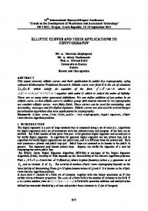
3. Determine the number of spaces by dividing the distance from the beginning to the end of the curve by the spacing value from the table and round this value to the nearest reasonable whole number, and 4. Determine the spacing distance of the chevrons by dividing the measured distance from the beginning to the end of the curve by the rounded number of spaces (19). A diagram of how the CTRE recommends placing of chevron signs and the table of spacings are located in Figure 1 and Table 3 respectively.

Figure 1. Diagram to Illustrate Placing of Chevron Signs on Curves (19).

20

Table 3. Suggested Spacing for Chevron Signs (19).

Overall, the results on whether or not chevrons are effective are mixed. However, according to Niessner’s study (25), there was a reduction in the number of run-off-the-road accidents where chevrons were used to delineate curves. In Jennings et. al.’s research, they found that chevrons reduced the speed and speed variance while following a horizontal curve (24). They also found that the chevrons caused drivers to follow the curve better. However, there are also results that state there were no significant results from using chevrons over other delineation methods. But given the results of the research, it can be determined that chevrons do provide some reduction in the speeds and speed variances and, therefore, add some safety for drivers. Most of the research discussed here used the MUTCD recommended spacing or two times the recommended spacing. Also, the research states that at least two or three must be in view of the driver at all times. Unfortunately, there was only one document that specified 21

spacings for chevrons in the form of an equation. However, some of the agencies and the studies used the post-mounted delineator spacings for those of chevrons as well. Table 4 shows an example of the mixed opinions and findings regarding spacing. The past research overall does not clearly show whether or not post-mounted delineators and chevrons improve safety on rural horizontal curves. There are mixed results for both methods but there appear to be more benefits from using post-mounted delineators or chevrons than not using them even though there is no trend one way or another from past research. The MUTCD needs to be more clearly defined, and more research should be done on what spacings will work the best for both chevrons and post-mounted delineators. Having two or three chevrons or post-mounted delineators “in view” of the driver throughout the curve is too vague and needs to be clarified so that there is no discrepancy on what is or is not “in view” of the driver. Using equations to specify the spacings may not be the best option, but perhaps a range of values depending on different configurations and sight-distance problems would provide more flexibility for rural curves that are not typical. More research should be done to determine what the minimum requirements are for post-mounted delineators and chevrons on a standard rural horizontal curve. Table 4. Chevron Spacing Summary. Recommended or studied spacing Reference Two in view MUTCD (22) Four in view Zwahlen and Park (23) Twice the recommended delineator spacing Jennings et. al (24) Three in view Zador et. al (5) Three in view Niessner (25) Two in view Roadway Delineation Practices Handbook (26) S = 4 . 5 R − 50 CTRE (19)

22

CHAPTER 3: STATE SURVEY TTI researchers developed and administered a state survey in order to determine how various states interpret some of the vague MUTCD language associated with the delineation of horizontal curves. Specifically, the survey was designed to determine if and when agencies interpret Section 3D.03 such that gentle horizontal curves on expressways and freeways can be considered tangent sections and, therefore, do not require delineation (as long as the appropriate exemptions from Section 3D.03 are satisfied), how agencies use and classify single and double delineators, and finally, how agencies expect their field crews to set the spacing for delineators and Chevrons. Figure 2 shows the survey instrument. It was sent to the state representatives on the American Association of State Highway and Transportation Officials (AASHTO) Maintenance Engineering subcommittee and the AASHTO Traffic Engineering subcommittee. A total of 34 states responded to the survey. The first question of the survey was aimed at determining whether agencies that use Retroreflective Raised Pavement Markings (RRPMs) on their freeways and expressways delineate gentle curves on these limited access facilities as tangents, and if so, at what point they make this distinction. This question was important because the wording of the MUTCD implies that all curves on freeways and expressways require post-mounted delineators, regardless of the radius. Twenty-seven states responded to this question. Of these, 17 states indicated that they do delineate horizontal curves as tangents at some point. The point at which a distinction is made ranged from a radius of 2865 ft (or a 2-degree curve) to 14,000 ft (or a 0.41-degree curve). The average was a radius of 6413 ft (or a 0.89-degree curve). The next question of the survey was aimed at determining whether there is a real need to distinguish between single and double delineators for various applications. Even though this was thought to be a minor issue, it is not hard to find delineators in the field that have the wrong number of reflector units on them.

23

The Texas Transportation Institute is conducting research for the Texas Department of Transportation regarding delineation practices along horizontal curves. The research is specifically focused on delineators and Chevrons. One of the objectives is to provide spacing guidelines for delineators and Chevrons that can be easily applied in the field without prior knowledge of curve radii or other features difficult to determine without a set of plans. I would be extremely grateful if you or one of your staff could take a few minutes to answer the following questions pertaining to the MUTCD and horizontal curve delineation. If you could, please respond by May 31.

1. Section 3D.03 implies that delineators are required on the right side of all curves on expressways and freeways. In many states such as Texas, RRPMs are used on lane lines such that the delineators are not needed on tangent sections of expressways and freeways. These types of facilities are also built to the highest standards, which translates to very gentle horizontal curvature. Does your agency interpret Section 3D.03 such that gentle horizontal curves may be considered tangent and therefore do not require delineators (as long as the appropriate exemptions of Section 3D.03 are satisfied)? If so, please indicate the point (i.e., radius or degree of curve) at which your agency delineates curves as tangent sections on expressways and freeways. For example, your agency may use the spacing table in the MUTCD (Table 3D1) which stops at 1000 ft radius curves (approximately 5.7 deg). If not, at what point (i.e., radius or degree of curve) would you consider acceptable practice to delineate an expressway or freeway curve as a tangent section? 2. Section 3D.03 indicates specific uses for single and double delineators. Does your agency distinguish between single and double delineators? Do you feel that it is necessary to distinguish between single and double delineators? How many classes of delineators does your agency use and what are their intended meanings? 3. Section 3D.04 provides guidelines for delineator spacing. The spacing depends on the radius or degree of curve. Does your agency use something other than radius or degree of curve to determine spacing? If not, how do your field personnel determine the pertinent information to select the appropriate spacing? Does your agency vary the approach and departure spacing as suggested in Section 3D.04? 4. Section 2C.10 addresses the Chevron sign. It says that Chevron spacing "should be such that the road user always has at least two in view . . ." How does your agency space Chevrons in horizontal curves? Please send your agency's related guidelines, practices, and/or specifications, particularly if they differ from the national MUTCD. Also, please include your name and phone number so that we may call you to follow up, if needed. Each response will be kept confidential in that only percentages and trends will ever be published as a result of this survey. Thank you, in advance, for your cooperation. contact me.

If you have any questions, please

Paul J. Carlson, Ph.D., P.E. Program Manager Texas Transportation Institute 3135 TAMU College Station, TX 77843-3135 PH: (979) 845-1728 FX: (979) 845-6006 Email: [email protected]

Figure 2. State Survey Instrument.

24

Thirty-two states responded to this question. Of these, 25 states reported that they do distinguish between single and double delineators. Only 12 states expressed their opinions regarding whether there was a need to make the single versus double delineator distinction. Interestingly, the results were split. The third question of the survey was designed to reveal the difficulty in applying the delineator spacing criteria as shown in the MUTCD. The MUTCD spacing table is based on the curve radius or degree of curve. While this may be adequate for the roadway design engineers, it is not convenient for field personnel who typically do not have easy access to this information or have a way to measure it in the field. Additionally, the MUTCD provides guidelines for variable delineator spacing on the approach and departure to horizontal curves. The states were asked if they practiced this guidance. Twenty-eight states answered this question. Of these, 26 states reported that they use either the curve radius or the degree of curve, exclusively. Two states reported that they use the advisory speed value of the curve to set the delineator spacing, and one other state reported that they use a constant spacing for all curves, regardless of the radius. Only seven of the 26 states that reported using either the curve radius of degree of curve to set delineator spacing in curves responded to the question of how their field personnel obtain the information (i.e., radius or degree of curve) to set the proper spacing. Surprisingly, three states reported that they use the chord method, which is a rather laborious and inaccurate procedure that puts the field personnel on the road to make the measurements (this method, and others, are more fully described in the following chapter). As reported above, two states use the advisory speed value and another uses constant spacing in all curves. Of the 28 states that responded, 19 reported that they use some form of variable delineator spacing on the approach and departure to horizontal curves. Some unique variations were provided. For instance, one state uses only one delineator on the approach and departure, and it is spaced as 2×S (where S is the spacing in the curve). Another state uses the MUTCD guidance but omits the third delineator on the approach and departure to the curve. Yet another practice reported by one of the states makes use of two delineators on the approach and departure, but their spacing is 2×S rather than 2S and then 3S (as per the MUTCD).

25

The fourth and final question of the survey focused on Chevron spacing in horizontal curves. The question was asked to determine if there are states using more objective spacing criteria than MUTCD’s guidance of having at least two in view. Half of the 32 states that responded to the Chevron spacing question reported that they use the MUTCD criteria of two in view. Three states reported that they use the same concept as the MUTCD criteria except they try to provide three in view. Three states use a table based on the advisory speed value to space Chevrons. Two states use the MUTCD delineator spacing table without modifications, and one state reported that they double the spacing of the MUTCD delineator spacing table for their Chevron spacing. Other states reported various formulas or radius-dependent tables. Appendix A shows the spacing tables that were provided by the states, for both delineators and Chevrons.

26

CHAPTER 4: STATE-OF-THE-PRACTICE One of the early fundamental issues associated with this research was determining the state-of-the-practice with respect to the installation and maintenance of delineators and Chevrons along horizontal curves. Therefore, TTI researchers visited horizontal curves on statemaintained highways to assess the current installation and maintenance practices used by TxDOT field crews. Researchers then compared the findings to TxDOT standards and guidelines. Part of the reason for these activities was to understand the current difficulties and to determine the potential for making improvements to the current practices. CURVE LOCATIONS AND CHARACTERISTICS Researchers visited 58 curves in various areas of Texas including the Bryan, Waco, Amarillo, and Atlanta Districts. One of the required curve characteristics was the presence of an advisory speed. Researchers used TxDOT Road Inventory Logs (RI logs) or as-built plans to identify or calculate geometric curve characteristics such as length, deflection angle, and radii. Traffic control characteristics, such as delineation type and spacing, and posted and advisory speed values were recorded at each location. Researchers also collected roadway characteristics such as number of lanes, width of lanes, and width of shoulders. Of the 58 curves, the advisory speed ranged from 15 mph to 65 mph, and the radii ranged from 180 ft to almost 2000 ft. MEASURED DELINEATOR SPACING In order to determine how delineators in the field were spaced and how that compared to the Texas MUTCD recommendations, the distance between the delineators was measured and then compared to the following Texas MUTCD criteria: “The spacing of delineators should be adjusted on approaches to and throughout horizontal curves so that several delineators are always simultaneously visible to the road user (2).” Table 5 shows the delineator spacing table from the Texas MUTCD (2). The recommended spacing on the approach of the curve in each direction is 2S for the first delineator just before the point of curvature (PC) or just after the point of tangency (PT) of the curve, 3S for the second delineator, and 6S for the third delineator (where S is the spacing in the curve). The

27

Texas MUTCD also recommends that delineator spacing should not be less than 20 ft or more than 300 ft. Table 5. Table 3D-1 from the Texas MUTCD. Radius of Curve (ft)

Approximate Spacing (S) on Curve (ft)

50

20

115

25

180

35

250

40

300

50

400

55

500

65

600

70

700

75

800

80

900

85

1000

90

As shown in Table 6, researchers collected data on 35 curves with delineators. None of the curves examined had delineators spaced at 2S, 3S, or 6S on the tangent approach or departure to or from the curve. On most of these curves, there was one delineator in advance of the point of curvature and beyond the point of tangency. All the curves had at least three delineators in view at any point on the curve. Table 6 also includes the average field spacing and the spacing recommended by the Texas MUTCD.

28

Table 6. Delineator Spacing as Measured in the Field.

Curve Locations FM 1671 FM 1404 FM 449 FM 168 FM 1860 FM 556 FM 285 FM 935 SH 207 9 (Armstrong, South) 1 2 3 4 5 6 7 8

SH 207 10 (Armstrong, Middle) 11 FM 159 SH 207 (Armstrong, 12 North) 13 FM 285 14 FM 293 (West) 15 FM 293 (East) 16 FM 46 17 FM 1258 (North) 18 FM 1258 (South) 19 FM 2300 20 FM 2161 (North) 21 FM1258 22 FM 2385 (East) 23 FM 2385 (West) 24 FM 2161 (South) 25 FM 1151 (East) 26 FM 1151 (West) 27 FM 1342 (West) 28 FM 294 29 FM 1342 (East) SH 207 30 (Carson, South) 31 FM 293 (East) 32 FM 293 (West) 33 FM 2386 (Middle) 34 FM 2386 (North) 35 FM 2386 (South)

Speed Limit (mph) Delineator Spacing Posted Advisory Change in Number of Average Standard Radius Speed Speed Speed Delineators Spacing Deviation Limit 60 25 35 6 133 9 190 55 35 20 11 90 25.6 320 55 35 20 10 80 57.2 441 55 35 20 21 66 14.7 500 60 40 20 11 96 10.2 567 60 40 20 15 100 49.6 573 55 40 15 28 72 40.8 574 55 40 15 9 114 34.6 637

Tx MUTCD Recommended Spacing 35 49 59 64 68 69 69 73

50

40

10

15

67

41.0

717

77

50 60

40 40

10 20

25 9

66 79

38.1 0.8

717 721

77 78

50 55 70 70 60 70 70 70 70 70 70 70 70 70 70 70 70 70

40 45 45 45 45 50 50 55 55 55 55 55 55 55 55 60 60 60

10 10 25 25 15 20 20 15 15 15 15 15 15 15 15 10 10 10

19 16 22 14 16 10 10 18 15 32 20 24 16 31 34 11 28 9

79 125 99 130 117 155 165 75 64 81 99 93 76 97 103 97 107 96

57.5 38.3 75.9 148.0 57.3 83.9 93.1 57.6 13.4 45.6 71.0 74.2 35.4 36.9 45.9 56.3 75.8 50.6

818 595 717 718 1027 960 1003 820 956 956 957 958 959 1143 1147 1145 1147 1155

83 70 77 78 94 90 93 83 90 90 90 90 90 99 99 99 99 100

70 70 70 70 70 70

60 65 65 65 65 65

10 5 5 5 5 5

11 4 4 11 7 11

154 135 133 103 181 115

63.2 50.5 1.89 30.1 164.6 48.8

1901 1425 1443 1906 1913 1916

129 111 112 129 129 130

The data in Table 6 show that the delineator spacing on the curves, on average, isfairly consistent with the guidelines in the MUTCD. On average, the difference was only 12 ft. However, there are some clear examples that show differences between the guidelines and field measurements of over 50 ft. Despite these differences, as Figure 3 shows, the curves all had 29

several delineators in view throughout the curve. At night, most of the delineators should be easily seen because of the reflective aspects of the delineator.

Figure 3. Example of Curve with Delineators.

MEASURED CHEVRON SPACING Data were collected on 15 curves with Chevrons. The distance between each Chevron was measured to identify any placement patterns in the field. In most cases, the Chevrons were spaced approximately equally. When a road intersected within a curve, a Chevron was often omitted. Table 7 shows several curve characteristics of the curves with Chevrons.

30

Table 7. Chevron Spacing as Measured in the Field.

1 2 3 4 5 6 7 8 9 10 11 12 13 14 15

Curve Locations FM 3090 Curve 1 FM 185 FM 974 Curve 2 FM 450 FM 852 FM 974 Curve 3 FM 1237 FM 1179 Curve 1 FM 3090 Curve 2 FM 1179 Curve 2 FM 487 Curve 2 FM 487 Curve 1 FM 2038 FM 2223 SH 207 (Carson, North)

Speed Limit (mph) Chevron Spacing (ft) Standard Change in Number of Average Posted Advis. Chevrons Deviation Speed 60 15 45 5 48 3.8 Unknown 25 4 91 25.7 60 30 30 5 93 3.5 55 30 25 7 83 29.5 55 30 25 8 74 29.9 60 30 30 5 75 4.6 60 35 25 7 119 34.8 65 35 30 2 124 N/A 60 35 25 5 78 7.4 65 35 30 3 195 43.1 55 40 15 6 136 32.7 55 40 15 6 135 26.9 70 45 25 5 177 20.8 70 50 20 5 188 3.8 70

60

10

9

100

0.9

Curve Radius 191 179 316 318 472 478 409 474 478 482 409 410 1142 958 1426

The data in Table 7 shows the average spacing between Chevrons. The Texas MUTCD and the FHWA MUTCD both recommend spacing Chevrons such that there are “at least two in view, until a change in alignment eliminates the need for the signs.” Therefore, there are no quantitative spacing guidelines to compare with the field data. Figures 4 and 5 show examples indicating that that the Chevron spacing on two of these curves meets the Texas MUTCD criteria of having at least two Chevrons in view (as did all of the sites visited). Researchers observed that the Chevrons were placed approximately at the point of curvature and ended at approximately the point of tangency. Researchers also discovered that there was a large difference between the Chevron spacing from district to district.

31

Figure 4. An Example of Chevrons along a Curve.

32

Figure 5. Another Example of Chevrons along a Curve. Figure 6 was developed to illustrate the relationship that exists between the radius and the average Chevron or delineator spacing from the data collected in the field. Figure 6 shows that Chevrons are almost exclusively reserved for curves with radii of 500 ft or less while delineators appear to be used more on curves above 500 ft radii. The other point here is that there is very little correlation between the radii of horizontal curves and the spacing that is used in the field. For the delineators, the coefficient of determination for the linear model shown was only 29 percent and for Chevrons the relation was even weaker (18 percent).

33

2500 Chevrons Delineators Linear (Chevrons)

2000

Curve Radius (ft)

Linear (Delineators)

1500

1000

500

0 0

40

80

120

160

200

Spacing (ft)

Figure 6. Chevron and Delineator Spacing versus Radius.

APPLICATION OF DELINEATORS Table 8 shows the TxDOT guidelines for curve delineation treatment use. These guidelines can be found in the Traffic Operations Manual - Signing & Markings Volume (28). Table 8. TxDOT Guidelines for Curve Treatments. Difference Between Posted Speed and Advisory Speed (mph) 0-14 15-24 25 and above

Recommended Curve Delineation Treatment RRPMs RRPMs and Delineators RRPMs and Chevrons

For curves with differences of less that 15 mph between the posted and advisory speed, TxDOT guidelines suggest the use of RRPMs for delineators, exclusively. All of the eight curves that the researchers visited with no delineators or Chevrons fell within this group.

34

However, 13 of the 35 curves with delineators had speed differences less than 15 mph and one of the 15 curves with Chevrons had a speed difference less than 15 mph. For curves with speed differences of 15 to 24 mph, the TxDOT guidelines suggest adding delineators to the RRPMs along the curves. Only 19 of the 35 curves visited by the researchers that had delineators fell within this criteria and three of the 15 Chevron curves fell into this criteria. On curves where the difference between the speed limit and the advisory speed is 25 mph or more, the TxDOT policy is to use Chevrons with RRPMs. Ten of the 15 curves with Chevrons fell into this group and two of the 35 curves with delineators fell into this category. MEASURED SUPERELEVATION Superelevation is an important feature of horizontal curves, not only in terms of countering lateral acceleration, but also when it comes to estimating radius, depending on the method of choice. For instance, ball bank indicators (BBI), which are typically used to determine advisory speed values, can also be used to estimate curve radius. However, superelevation is an important factor because it affects the ball bank indicator reading. The ball bank indicator reading (α) is the result of the combined effects of the lateral acceleration angle (θ), the superelevation angle (φ), and the body-roll angle (ρ). The equation for the BBI reading is: α = θ − φ + ρ. This equality and its use to estimate horizontal curve radius is further explained in Chapter 5. The superelevation was measured along a sample of the visited curves in the Bryan and Waco Districts so that an understanding of the variation could be developed as this is an important aspect to the determination of radius using ball bank indicators. The hope was to eventually develop an empirical relationship that could be used to estimate superelevation so that it would not need to be measured but would still provide a reasonably accurate value if needed. Researchers measured the superelevation at each chevron or delineator. The superelevation was measured every 200 ft on curves that only had curve warning signs and advisory speed plates. The average superelevation was calculated on each curve by visually inspecting the superelevation profile and averaging the superelevation measurements that seemed to represent full superelevation. Figure 7 illustrates this method. The point of curvature and the point of tangency are placed in an estimated position based on the length of the curve calculated from the RI log and the distance between the third and seventh delineators. 35

Superelevation (%)

10 8 6 4 2 0 -2 -4 -6 -8 -10 -12

PC

0

200

PT

400

600

800

1000

1200

Distance (ft) - Super

+ Super

Figure 7. Superelevation within the Curve on FM 1860. Figure 7 shows an example of how the superelevation on a curve changes as a function of distance. The positive superelevation measurements are approximately what one would expect to see. Slightly in advance of and just after the beginning of the curve, the road would be approaching full superelevation (i.e., be in superelevation run out [SRO]). At approximately the third delineator, the superelevation starts to flatten out. The third through seventh delineators seem to make up the plateau (full superelevation), and then the superelevation begins to approach normal -2 percent grade. The average superelevation calculation is an average of the delineator superelevation measurements that appear to be at full superelevation. These averages were calculated for each curve, and the data are given in Tables 9 and 10. The negative superelevation measurements for this curve illustrate an additional point. While many superelevation profiles observed appeared to follow the expected pattern, there were also several cases where there was variation in the superelevation measurements. This result is not surprising. Uneven settlement or wear on pavements could account for this type of variation. However, this outcome makes it difficult to form statistically valid predictions for superelevation. Figures 8 and 9 present the data graphically. 36

Table 9. Average Superelevation on Curves in the Bryan District. Bryan District Curves FM 1179 Curve 1 FM 1179 Curve 2 FM 2223 FM 974 Curve 2 FM 974 Curve 3 FM 2038 FM 159 FM 3090 Curve 1 FM 3090 Curve 2 FM 46

Speed Limit Curve Attributes Average Posted Advis. Change Length RRILOG Delin. 1 Speed Speed in Speed Low2 High (ft) (ft) (Device) 65 35 30 417 474 Chev. Curve too short. 65 35 30 444 482 Chev. Curve too short. 70 50 20 766 958 Chev. 2.6 -6.1 60 30 30 496 316 Chev. 5.8 -11.0 60 30 30 528 478 Chev. 5.5 -7.9 70 45 25 940 1142 Chev. 3.4 -6.1 60 40 20 343 721 Delin. 3.9 -5.2 60 15 45 248 191 Chev. 8.2 -8.0 60 35 25 597 478 Chev. 6.5 -7.3 60 45 15 950 1027 Delin. 5.0 -7.0

Superelevation Standard Deviation High1

Low2

1.7 1.4 0.8 1.4 0.5 0.4 0.9 1.2

1.0 2.3 0.4 2.0 0.0 0.4 0.6 1.1

emin

emax

High1 Low2 High1 Low2

1.2 4.3 4.8 2.0 3.4 7.9 5.9 3.4

-6.9 -13.7 -8.4 -8.4 -5.2 -8.4 -7.7 -5.7

4.5 7.0 6.3 10.2 4.3 8.7 7.5 6.3

-4.9 -9.3 -7.6 -18.3 -5.2 -7.7 -6.6 -8.5

1. High side of curve, positive superelevation. 2. Low side of curve, negative superelevation. Table 10. Average Superelevation on Curves in the Waco District. Waco District Curves FM 487 Curve 1 FM 487 Curve 2 FM 1237 FM 935 FM 1860 FM 2086 FM 2113 FM 2311

Speed Limit Curve Attributes Posted Advis. Change Length RRILOG Delin. Speed Speed in Speed (ft) (ft) (Device) 55 40 15 644 410 Chev. 55 60 55 60 60 60 60

40 35 40 40 50 55 55

15 25 15 20 10 5 5

649 649 644 544 1014 961 496

409 409 410 567 637 956 955

Chev. Chev. Delin. Delin. Ad. Spd Ad. Spd Ad. Spd

1. High side of curve, positive superelevation. 2. Low side of curve, negative superelevation.

37

Average

Superelevation emin Standard Deviation

High1 4.1

Low2 -6.1

High1 0.4

Low2 1.1

6.7 5.0 5.5 7.1 6.9 5.2 6.1

-8.3 -6.7 -8.6 -8.0 -9.5 -4.8 -10.2

1.2 1.0 0.7 0.4 0.7 0.9 0.1

0.5 0.8 1.6 1.2 1.6 1.1 0.6

emax

High1 Low2 High1 Low2 3.8 -4.7 4.6 -7.1 5.4 3.9 4.7 6.5 5.9 4.0 6.0

-7.7 -5.4 -7.2 -6.5 -8.2 -3.6 -9.8

8.1 6.2 6.4 7.4 7.6 5.9 6.1

-9.0 -7.4 -10.8 -9.4 -11.6 -6.2 -10.6

Average Full Superelevation (%)

10 8 6 4 2 0 -2 -4 -6 -8 -10 -12 0

200

400

600

800

1000

1200

50

60

Radius (ft) Positive superelevation

Negative superelevation

Figure 8. Radius versus the Average Superelevation.

Average Full Superelevation (%)

10 8 6 4 2 0 -2 -4 -6 -8 -10 -12 0

10

20

30

40

Advisory Speed (mph) Positive superelevation

Negative superelevation

Figure 9. Advisory Speed versus the Average Superelevation.

38

BBI COMPARISON For a sample of the curve visited, researchers obtained ball bank indicator measurements from three different BBI instruments simultaneously. The rational behind using three instruments was to determine if they provided consistent results. Figure 10 shows a photograph of all three instruments. The top ball bank indicator in Figure 10 was a Rieker manual ball bank indicator. It is the standard BBI issued from the TxDOT warehouse. Besides the low resolution markings on this device, another drawback is that it requires two people to set the advisory speed – one person to drive and the other to read the ball bank indicator. A solution to this problem is the electronic ball bank indicator, the bottom BBI shown in Figure 10, which has been used by some districts in TxDOT. An advantage of the electronic ball bank indicator is that it can be set to audibly alert the driver when the ball bank indicator reading exceeds 10 degrees; therefore, it only requires one person to set advisory speeds on curves. The third ball bank indicator was a Slopemeter manual ball bank indicator, the middle BBI in Figure 10. It is larger than the Rieker manual BBI, and tick marks denote every degree between -28 and +28. The larger face and additional tick marks made this instrument easier to read than the Rieker manual.

39

Figure 10. Ball Bank Indicators. (from top: Rieker Manual, Slopemeter, Rieker Electronic) The ball bank indicator data were compared to identify any differences between the three instruments. Tables 11 and 12 show the ball bank indicator data for each instrument and the linearly interpolated speed at a ball bank indicator reading of 10 degrees.

40

Table 11. Ball Bank Indicator Data for the Curves in the Bryan District. Velocity* Curve (mph) Location Brazos Co. FM 1179 Curve 1

FM 1179 Curve 2

FM 2223

FM 974 Curve 2

FM 974 Curve 3

FM 2038

FM 159

30 35 40 45 30 35 40 45 45 50 55 60 65 25 30 35 40 45 25 30 35 40 45 40 45 50 55 60 35 40 45 50 55

Slopemeter (degrees) NEB 5 9 12 18 -5 -8 -12 -18 NB -8 -11 -12 -16 -18 NB 5 9 14 19 25 NB -3 -5 -6 -10 -15 NB -5 -7 -8 -11 -14 NB -5 -7 -10 -12 -15

SWB -5 -8 -12 -16 5 8 11 17 SB 8 10 13 14 17 SB -4 -7 -11 -17 -24 SB 5 5 9 14 19 SB 6 7 11 12 14 SB 6 7 11 14 16

BBI =10 ° (mph) NEB SWB 36

37

37

37

NB

SB

49

50

NB

SB

31

32

39

34

NB

SB

52

50

NB

SB

45

44

Rieker Mech. (degrees) NEB 5 8 12 18 -5 -8 -12 -17 NB -7 -10 -12 -15 -18 NB 5 8 12 18 +20 NB -3 -4 -6 -10 -15 NB -5 -7 -8 -11 -13 NB -4 -7 -9 -11 -15

41

SWB -5 -9 -12 -15 5 9 12 17 SB 7 11 13 16 19 SB -4 -7 -11 -16 +20 SB 4 5 8 12 18 SB 6 7 10 11 13 SB 5 7 10 13 15

BBI =10 ° (mph) NEB SWB 37

37

37

37

NB

SB

51

50

NB

SB

32

33

39

36

NB

SB

53

52

NB

SB

47

45

Rieker Digital (degrees) NEB 4 7 11 14 -5 -9 -13 -14 NB -8 -10 -12 -16 -20 NB 3 7 10 18 23 NB -2 -4 -6 -9 -15 NB -5 -7 -11 -13 -13 NB -4 -7 -9 -11 -14

SWB -6 -8 -11 -15 5 5 11 14 SB 8 9 13 14 17 SB -3 -7 -11 -16 -23 SB 2 3 8 12 16 SB 4 5 9 11 15 SB 5 7 8 11 14

BBI =10 ° (mph) NEB SWB 39

38

37

39

NB

SB

50

50

NB

SB

33

33

NB

SB

39

37

NB

SB

50

52

NB

SB

47

47

Table 11 Continued. Velocity* Curve (mph) Location Grimes Co. FM 3090 Curve 1

FM 3090 Curve 2

Slopemeter (degrees)

25 30 35 40 45

NB -4 -7 -11 -22 NB -5 -10 -10 -15 -18

SB 2 5 10 20 SB 6 10 11 16 18

35 40 45 50 55

NB -5 -7 -10 -14 -17

SB 6 10 13 16 20

15 20 25 30

Ball Bank Indicator Data BBI =10 ° Rieker Mech. BBI =10 ° (mph) (degrees) (mph) NB

SB

22

23

NB

SB

33

31

NB -3 -7 -10 -20 NB -5 -10 -10 -14 -18

SB 2 5 9 20 SB 6 10 10 15 18

NB -4 -6 -9 -13 -15

SB 5 9 12 15 19

NB

SB

23

23

NB

SB

33

32

Rieker Digital (degrees) NB -3 -7 -11 -19 NB -5 -10 -14 -18

SB 2 3 7 17 SB 5 7 9 13 15

NB -4 -8 -9 -14 -16

SB 6 8 10 13 18

BBI =10 ° (mph) NB

SB

23

25

NB

SB

35

35

NB

SB

45

43

Robertson Co.

FM 46

NB

SB

44

41

* Bold italicized speeds represent the posted advisory speed.

42

NB

SB

46

42

Table 12. Ball Bank Indicator Data for Curves in the Waco District. Curve Location FM 2086

FM 1237

FM 1860

FM 2113

FM 2311

Velocity* (mph) 45 50 55 30 35 40 45 35 40 45 50 55 50 55 60 50 55 60 65

FM 487 Curve 1

35 40 45

FM 487 Curve 2

35 40 45

FM 935

35 40 45 50

Slopemeter (degrees) EB WB -12 13 -15 16 -21 19 EB WB 9 -9 14 -10 17 -14 22 -17 NB SB -5 6 -8 10 -11 15 -15 17 -19 23 EB WB 9 -10 13 -14 15 -16 NB SB 9 -7 11 -12 14 -12 17 -14 WB EB -9 10 -13 15 -16 20 WB EB 10 -8 15 -12 18 -17 WB EB -8 11 -12 17 -16 20 -21 27

BBI =10 ° (mph) EB WB 44

40

EB

WB

31

33

NB

SB

43

40

EB

WB

51

50

NB

SB

52

55

WB

EB

36

35

WB

EB

35

37

WB

EB

38

34

Rieker Mech. (degrees) EB WB -11 12 -14 15 -19 18 EB WB 10 -8 13 -10 16 -13 -17 NB SB -4 6 -7 9 -11 14 -15 16 -18 21 EB WB 8 -9 11 -13 14 -14 NB SB 8 -7 11 -10 13 -11 17 -13 WB EB -9 10 -12 14 -16 19 WB EB 9 -8 13 -12 17 -16 WB EB -7 10 -11 16 -16 20 -20 +20

BBI =10 ° (mph) EB WB 44

42

EB

WB

37

34

NB

SB

44

41

EB

WB

53

51

NB

SB

54

57

WB

EB

37

35

WB

EB

36

38

WB

EB

39

35

Rieker Digital (degrees) EB WB -14 11 -14 13 -19 16 EB WB 7 -9 11 -10 14 -14 18 -17 NB SB -5 5 -8 9 -9 13 -14 14 -18 0 EB WB 7 -10 10 -13 12 -15 NB SB 7 -8 10 -11 12 -11 15 -13 WB EB -9 8 -13 13 -15 17 WB EB 7 -8 12 -12 16 -16 WB EB -8 9 -13 14 -17 17 -21 25

BBI =10 ° (mph) EB WB 42

43

EB

WB

34

33

NB

SB

44

45

EB

WB

56

50

NB

SB

56

55

WB

EB

36

37

WB

EB

38

38

WB

EB

37

37

* Bold italicized speeds represent the posted advisory speed. In most cases, the ball bank indicator readings are within two degrees when different instruments were compared at the same speed and in the same direction on a curve. This translates into a one to two mph difference between the interpolated speeds. There are only a few cases where there is more than a two mph difference between the interpolated speeds. The differences in the ball bank indicator readings appear random. There is no indication that one instrument is consistently higher or lower than another. 43

ADVISORY SPEED VALUE VERSUS BALL BANK INDICATOR This section of the report discusses the research activities performed to determine whether the advisory speed values were appropriately set along the curves visited by the researchers. Advisory speeds are set by driving trial runs around a curve starting at five mph less than an estimated safe speed. The sequential runs are driven at five mph greater than the previous run until the ball bank indicator meets or exceeds 10 degrees. The advisory speed is then set at the speed at which the ball bank indicator reads 10 degrees or five mph less than the speed at which the ball bank indicator first exceeded 10 degrees. Ten degrees is considered a safe and comfortable ball bank indicator reading limit. Using the three BBI devices described in the previous section, researchers collected BBI data on 10 curves in the Bryan District and eight curves in the Waco District. All BBI data were collected in a 2000 Ford Taurus. The ball bank indicator data were plotted at each speed. Tables 11 and 12 in the previous section provide a complete set of the ball bank indicator data collected, as well as the interpolated speed at a ball bank indicator reading of 10 degrees. This interpolation was computed twice for each curve, once using the data from the high side of the curve (the outside of the curve, positively superelevated) and once using the data from the low side of the curve (the inside of the curve, negatively superelevated). The interpolated speed was then used to determine if the advisory speed had been set appropriately. Researchers deemed the advisory speed appropriately set in both directions if the linearly derived speed at 10 degrees was greater than or equal to the advisory speed and less than the advisory speed plus five mph. It could be argued that using one advisory speed per curve (i.e., one advisory speed for both directions on the curve) is what motorists expect so the advisory speed should be considered appropriately set if one direction is correct, but the advisory speed in the opposite direction is lower than the appropriate advisory speed for the first direction. Tables 13 and 14 show a list of the curves for each district and whether each curve is set appropriately on each side of the curve based on the criteria in the above paragraph. The last column shows if the advisory speed is set appropriately for both sides of the curve. The advisory speed is considered to be set appropriately for both sides of the curve if one side of the curve, based on the criteria in the previous paragraph, is set appropriately and the other side of the curve is considered to have been set low. If, however, the advisory speed for either direction was set too high, the advisory speed

44

was considered too liberal, and thus, did not meet the “appropriately set” criteria for the column labeled “Both.” Table 13. Advisory Speed Set Appropriately for Both Directions (Curves in Bryan District)?

Curve Location 1 FM 1179 Curve 1 Slopemeter Rieker Mech. Rieker Digital 2 FM 1179 Curve 2 Slopemeter Rieker Mech. Rieker Digital

Interpolated Appropriate Interpolated Appropriate Appropriate BBI Reading: Advisory BBI Reading: Advisory Advisory 10 Degrees 10 Degrees Speed Speed Speed (High Side) (High Side)? (Low Side) (Low Side)? (Both Sides)?

37 37

Advisory Speed: Yes 37 Yes 37 Yes 38 Advisory Speed: Yes 37 Yes 37

39

Yes

36 37 39

3 FM 2223 Slopemeter

4

5

6

7

Rieker Mech. Rieker Digital FM 974 Curve 2 Slopemeter Rieker Mech. Rieker Digital FM 974 Curve 3 Slopemeter Rieker Mech. Rieker Digital FM 2038 Slopemeter Rieker Mech. Rieker Digital FM 159 Slopemeter Rieker Mech. Rieker Digital

37

Yes Yes

35 mph Yes Yes Yes 35 mph Yes Yes

Yes

Yes

Yes Yes Yes

Advisory Speed: 50 50 50 31 32 33 34 36 37 50 52 52 44 45 47

Yes 49 Yes 51 Yes 50 Advisory Speed: Yes 32 Yes 33 Yes 33 Advisory Speed: Yes 39 LOW 39 39 LOW Advisory Speed: LOW 52 LOW 53 LOW 50 Advisory Speed: Yes 45 LOW 47 47 LOW

45

50 mph HIGH Yes Yes Yes Yes Yes LOW LOW LOW LOW LOW LOW LOW LOW LOW

HIGH Yes Yes 30 mph Yes Yes Yes 30 mph Yes LOW LOW 45 mph LOW LOW LOW 40 mph Yes LOW LOW

Table 13. Continued.

Curve Location 8 FM 3090 Curve 1 Slopemeter Rieker Mech. Rieker Digital 9 FM 3090 Curve 2 Slopemeter Rieker Mech. Rieker Digital 10 FM 46 Slopemeter Rieker Mech. Rieker Digital

Interpolated Appropriate Interpolated Appropriate Appropriate BBI Reading: Advisory BBI Reading: Advisory Advisory Speed 10 Degrees Speed 10 Degrees Speed (High Side) (High Side)? (Low Side) (Low Side)? (Both Sides)? Advisory Speed: 15 mph 23 LOW 22 LOW LOW 23 LOW 23 LOW LOW 25 LOW 23 LOW LOW Advisory Speed: 35 mph 36 Yes 38 Yes Yes 37 Yes 38 Yes Yes 40 LOW 37 Yes Yes Advisory Speed: 45 mph 41 HIGH 49 Yes HIGH 42 HIGH 51 LOW HIGH HIGH 43 HIGH 50 LOW

46

Table 14. Advisory Speed Set Appropriately for Both Directions (Curves in Waco District)?

Curve Location 1 FM 487 Curve 1 Slopemeter Rieker Manual Rieker Digital 2 FM 487 Curve 2 Slopemeter

3

4

5

6

7

8

Rieker Manual Rieker Digital FM 1237 Slopemeter Rieker Manual Rieker Digital FM 935 Slopemeter Rieker Manual Rieker Digital FM 2086 Slopemeter Rieker Manual Rieker Digital FM 2113 Slopemeter Rieker Manual Rieker Digital FM 2311 Slopemeter Rieker Manual Rieker Digital FM 1860 Slopemeter Rieker Manual Rieker Digital

Interpolated Appropriate Interpolated Appropriate Appropriate BBI Reading: Advisory BBI Reading: Advisory Advisory 10 Degrees Speed 10 Degrees Speed Speed (High Side) (High Side)? (Low Side) (Low Side)? (Both Sides)? 34 34 42 35 36 37 31 30 34 34 35 37 40 42 43 51 53 56 50 50 54 40 41 42

Advisory Speed: HIGH 37 HIGH 38 Yes 38 Advisory Speed: HIGH 37 HIGH 38 HIGH 38 Advisory Speed: HIGH 33 HIGH 34 HIGH 33 Advisory Speed: HIGH 38 HIGH 39 HIGH 37 Advisory Speed: HIGH 44 HIGH 44 HIGH 42 Advisory Speed: HIGH 50 HIGH 51 Yes 50 Advisory Speed: HIGH 60 HIGH 60 HIGH 60 Advisory Speed: Yes 43 Yes 44 Yes 44

HIGH HIGH HIGH HIGH HIGH HIGH HIGH HIGH HIGH HIGH HIGH HIGH HIGH HIGH HIGH HIGH HIGH HIGH Yes LOW Yes Yes Yes Yes

40 mph HIGH HIGH HIGH 40 mph HIGH HIGH HIGH 35 mph HIGH HIGH HIGH 40 mph HIGH HIGH HIGH 50 mph HIGH HIGH HIGH 55 mph HIGH HIGH HIGH 55 mph HIGH HIGH HIGH 40 mph Yes Yes Yes

Out of the total number of curves examined, researchers found that about 29 percent set appropriately by all three ball bank indicators. Researchers also found that approximately 47 percent of the curves examined were considered to be set appropriately by at least one ball bank indicator.

47

Some curves were set appropriately in one direction, but not in the other direction. This could be caused by several factors including uneven pavement surfaces on one side of the road, or inconsistent path driven by the researcher. A third reason for differing interpolated advisory speeds is the high side of the curve has a larger radius than the low side of the curve; thus, the low side of the curve is a tighter curve, and a lower advisory speed could be expected. However, a close comparison between the interpolated advisory speed on the high side of the curve and the interpolated advisory speed on the low side of the curve indicates the low side of the curve has a higher interpolated advisory speed for several different curves. FM 2311 and FM 935 are both examples of this result (see Table 12). Since this result was counterintuitive, researchers examined the superelevation characteristics for these curves. Tables 15 and 16 list the average superelevation on the high side and the low side for each curve. These tables also list the absolute value of the difference between the high side superelevation and the low side superelevation. In some cases, for example FM 2311 and FM 935, the large difference between the high side superelevation and the low side superelevation is likely the reason the interpolated advisory speed on the low side of the curve is higher than the interpolated advisory speed on the high side of the curve. Table 15. Difference between Average Superelevation on the High Side and the Low Side of the Curve for Curves in the Bryan District. Curve Location Bryan District FM 1179 Curve 1 FM 1179 Curve 2 FM 2223 FM 974 Curve 2 FM 974 Curve 3 FM 2038 FM 159 FM 3090 Curve 1 FM 3090 Curve 2 FM 46

Speed Limit (mph) Curve Attributes Change Length RRILOG Delin. Posted Advis. in Speed (ft) (ft) (device) 65 35 30 417 474 Chev. 65 35 30 444 482 Chev. 70 50 20 766 958 Chev. 60 30 30 496 316 Chev. 60 30 30 528 478 Chev. 70 45 25 940 1142 Chev. 60 40 20 343 721 Delin. 60 15 45 248 191 Chev. 60 35 25 597 478 Chev. 60 45 15 950 1027 Delin.

48

Superelevation (%) Average Difference High Low 2.6 2.0 -4.6 3.2 -5.3 2.1 2.6 -6.1 3.4 5.8 -11.0 5.2 5.5 -7.9 2.4 3.4 -6.1 2.7 3.9 -5.2 1.3 0.2 8.2 -8.0 6.5 -7.3 0.8 5.0 -7.0 1.9

Table 16. Difference between Average Superelevation on the High Side and the Low Side of the Curve for Curves in the Waco District. Curve Location Waco District FM 487 Curve 1 FM 487 Curve 2 FM 1237 FM 935 FM 1860 FM 2086 FM 2113 FM 2311

Speed Limit (mph) Curve Attributes Change Length RRILOG Delin. Posted Advis. in Speed (ft) (ft) (device) 55 40 15 644 410 Chev. 55 40 15 649 409 Chev. 60 35 25 649 409 Chev. 55 40 15 644 410 Delin. 60 40 20 544 567 Delin. 60 50 10 1014 637 Ad. Spd 60 55 5 961 956 Ad. Spd 60 55 5 496 955 Ad. Spd

Superelevation (%) Average Difference High Low 2.0 4.1 -6.1 1.6 6.7 -8.3 1.8 5.0 -6.7 3.1 5.5 -8.6 0.9 7.1 -8.0 2.5 6.9 -9.5 0.4 5.2 -4.8 4.2 6.1 -10.2

It should also be noted from Tables 15 and 16 that large differences between the superelevation of the high and low side of the curve do not always have as obvious an effect on the advisory speed as it does on FM 2311. For example, the difference between the high and low side superelevation on curve 2 on FM 974 is 5.2 percent; however, the difference between the advisory speeds for the high and low side of the curve was at most 1 mph (depending on which ball bank indicator instrument was used). In many cases, only a 1 to 2 mph difference was noted when the absolute value of the superelevation on the low side of the curve was greater than the superelevation on the high side of the curve.

49

CHAPTER 5: PILOT STUDIES This chapter presents the methods used to estimate radius. Early in the project, the researchers brainstormed to identify methods that could be used to estimate horizontal curve radius. The criteria that had to be satisfied in order for the researchers to consider the radius estimating method were only that they had to be safe and easy to implement, and preferably low cost. Table 17 shows the initial list of potential methods with brief descriptions. Table 17. Preliminary Methods to Estimate Curve Radius. Method Ball Bank Indicator 1 Ball Bank Indicator 2 Lateral Acceleration 1 Lateral Acceleration 2 Advisory Speed Value Yaw Rate Transducer Compass Chord Length GPS

Brief Description Use theoretical curve dynamic relationships to estimate the radius using speed and measured ball bank indicator readings. Assume superelevation and neglect bodyroll. Use an empirical relationship between speed and measured ball bank indicator readings to estimate radius. Assume superelevation and account for bodyroll in derived empirical relationship. Use theoretical curve dynamic relationships to estimate the radius using speed and measured lateral acceleration. Assume superelevation and neglect bodyroll. Same as Lateral Acceleration #1 method except this method includes a measurement of bodyroll and superelevation. Derive an empirical relationship between advisory speed value and radius. Measure deflection angle of curve using a yaw rate transducer and simultaneously measure length of curve with a distance measuring device. Calculate radius. Same as Yaw Rate Transducer method except this method is done with a compass. Stretch a known length of chord along an arc concentric to the radius. Measure the offset at the midpoint. Calculate radius. Use data that can be acquired from Global Positioning System (GPS) while driving a curve to determine radius.

Although the first five methods listed in Table 17 depend on the superelevation and bodyroll of the vehicle, they do not require personnel to get out of the vehicle. Therefore, safety is not compromised using these methods to estimate radius. In fact, the only two methods that require field personnel to leave their vehicle were the Compass and Chord Length methods. Consequently, because of safety, these methods were eliminated from further consideration. The

51

remaining methods were explored further to determine their feasibility with respect to TxDOT’s needs. The remainder of this chapter describes each of the curve estimating methods that were tested. Specifically, the methods for estimating the radius are described as well as the results that were obtained. It should be noted that the curves that were tested were the same ones as those used to determine the state-of-the-practice. A final section of this chapter compares the field spacing as measured and described in the previous chapter to the theoretical spacing if the methods explored in this chapter would have been implemented. This comparison demonstrates the potential usefulness of these methods compared to the status quo. BALL BANK INDICATOR METHODS The ball bank indicator is the most commonly used device to select a posted advisory speed on existing horizontal curves. In a recent survey, 88 percent of the states, cities, and counties that responded indicated that they use the ball bank indicator to set safe speeds (29). Therefore, if a method could be determined to estimate radius using the ball bank indicator, no additional equipment purchase would be needed. Combined with its ease of use, it was initially thought that a curve estimating radius method using a ball bank indicator had a lot of promise. The ball bank indicator is a curved level that when properly mounted in a vehicle measures the combined eaffects of the body roll angle (ρ), lateral acceleration angle (θ), and superelevation angle (φ). The relationship between the ball bank indicator reading and the aforementioned angles can be expressed by the following equation: Equation 1:

α=θ−φ+ρ

where: α = ball bank indicator reading, (degrees) ρ = body roll angle, (degrees) φ = superelevation angle, (degrees) θ = lateral acceleration angle. (degrees) In order to understand how the ball bank indicator reading can be used to estimate radius, it is important to review the fundamentals of horizontal curve design.

52

Horizontal Curve Design As a particle moves in a circular path of constant radius with constant speed, the acceleration is directed toward the center of the circle, perpendicular to the instantaneous velocity. This is called centripetal acceleration and is equivalent to the instantaneous normal acceleration, or: a⊥ =

Equation 2:

ν2 R

where: az = centripetal acceleration, (m/s2) v = speed of vehicle, (m/s) R = radius of horizontal curve, (m) According to Newton's second law (ΣF=ma), the acceleration must be caused by a force also directed toward the center of the curve. The net radial force on a particle of mass (m) traveling in uniform circular motion is: Equation 3:

F = ma ⊥ = m

ν2

where:

R

F = net radial force, (N=kg@m/s2) m = mass of vehicle, (kg) The centripetal acceleration shown in Equation 2 is referred to as lateral acceleration in highway engineering. Lateral acceleration is generated as a vehicle negotiates a horizontal curve with constant radius and is counterbalanced by the vehicle weight component related to the roadway superelevation and/or the side friction developed between the tires and pavement surface. The point mass model is used by the Green Book (30) to determine the minimum radius of a curve for a specified superelevation so that the lateral acceleration is kept within comfortable limits. On a superelevated curve, the superelevation offsets a portion of the lateral acceleration, such that: Equation 4:

a net =

ν2 - e

127 R 100

where:

53

anet = unbalanced lateral acceleration in g=s, (9.807 m/s2) e = superelevation in percent, (m/m) The unbalanced portion of lateral acceleration of the vehicle is a measure of the forces acting on the vehicle that tend to make it skid off the road (31). Using Newton's second law, the point mass model used to represent vehicle operation on a horizontal curve is the following: Equation 5:

e ν2 +f= 100 127 R

The left-hand side of Equation 4 represents the amount of lateral acceleration supplied while the right-hand side is the demanded lateral acceleration. In other words, the side friction demand of the vehicle is mathematically equivalent to the unbalanced lateral acceleration (anet). The tendency of the vehicle to skid must be resisted by tire/pavement friction. The vehicle will skid off the road unless the tire/pavement friction coefficient exceeds the side frictional demand. The side friction factor, f, of the supplied lateral acceleration is based on perceived vehicle occupants’ tolerable limits and is far below the threshold of tipping or sliding out for a typical passenger car. Therefore, if it were not for the body-roll angle, the ball bank indicator reading would be a direct measure of lateral acceleration. In other words, α from the ball bank indicator would be equal to the side friction factor f used in the point mass equation of the Green Book. A criticism of the ball bank indicator=s usage for setting safe speeds on existing curves is the influence of the test vehicle=s body-roll. A comprehensive study of the ball bank indicator (9) concluded that “The extreme effect of the body-roll of various model and makes of cars is only about 1 degree in the ball bank angle and provides a difference of about 2 km/h (3 mph) in speed.” The report recommended neglecting the body-roll influence as long as “The observers understand the effect of body-roll and make due allowance for it in case cars with extreme values are used for the driving tests.” However, according to the Green Book, “A correction must be made for that portion of force taken up in the small body-roll.” Therefore, due to the uncertainty of the influence of body-roll, this research also investigated the significance of body-roll and how it affects the reading of the ball bank indicator.

54

Ball Bank Indicator Method 1 This method is referred to as the physics ball bank indicator method from hereon after because it is based on the laws of physics. This method neglects the body-roll angle, and, if deemed promising, would require some sort of empirically derived assumption for the superelevation component. Because of the dismissal of body-roll, the ball bank indictor reading, α, equals the side friction factor, f, of the point mass model used in highway design to determine horizontal curve radius. If the speed of the vehicle and the ball bank indicator value are both simultaneously known, then the radius can be calculated using the following relationship: Equation 6:

R=

V2 15(e + f )

where: R = radius, (ft) e = superelevation, (ft/ft) and f = side friction factor (ft/ft) = ball bank indicator reading (α). It is important to note that this method relies on the superelevation. For the pilot testing of the method, the researchers measured the superelevation. If this method proved promising and worth fully developing, the researchers anticipated the need to develop an empirical relationship to minimize the error associated with guessing the superelevation. Initial, but unexplored, thoughts were setting the superelevation to a single value such as an average value or developing a relationship between superelevation and strongly correlated factors such as highway type, speed limit, or advisory speed value. Justification for neglecting the body-roll angle is provided by Moyer and Berry (32). They recommended neglecting body-roll because “the extreme effect of body-roll of various models and makes of cars is only about 1 degree in the ball bank indicator.” It should be noted that this conclusion was made in the 1940s when vehicles had much looser suspensions than today’s typical vehicles. More recent justification was provided in 1999 by Carlson and Mason (31). These researchers concluded that “. . . the results indicate that body-roll does not significantly influence the readings provided by the ball bank indicator.” Because all the data for the project reported in this report were collected using one type of vehicle, a 1998 Ford Taurus 55

from the TTI fleet, there is little reason to suspect that body-roll would play a significant part in the errors. Researchers collected ball bank indicator data using all three different types of ball bank indicators described in Chapter 4. The ball bank indicators were mounted to a wooden board and secured in the front seat between the driver and passenger seats. One person sat in the back seat and recorded the three ball bank indicators as the driver traversed each test curve. The curve was driven at the advisory speed, and four more times: at the advisory speed minus 5 mph, plus 5 mph, plus 10 mph, and plus 15 mph (only if the driver felt safe). The estimated radius was calculated using the data collected at each speed and for each direction of travel. Thus, the estimated radius at each speed were summed and averaged for each direction. The final average is an average of the radii from both directions at all of the data collection speeds. Table 18 is included to as an example of the calculations described. Table 18. Radius Estimation of Calculations for Curve 1 on FM 1179. Velocity

BBI readings

(mph)

(degrees) Slopemeter NB SB 5 -5 9 -8 12 -12 18 -16

30 35 40 45

Average Superelevation (percent) NB 2.0 2.0 2.0 2.0

SB -4.6 -4.6 -4.6 -4.6

Directional Average: Final Average:

Radius (feet) NB 642.9 482.3 471.3 396.7

SB 371.1 373.4 361.9 364.2

498.3

367.6 433.0

In Table 18, the radius is calculated using Equation 6. Body-roll is ignored for the physics method, so the side friction factor is assumed to be the ball bank indicator reading converted into radians. Average superelevation is also converted to radians for radius estimates. The dashed line box represents the radius estimates included in the final average calculation. The solid line boxes represent the radius estimates that are included in the directional average calculation. The measure of effectiveness was how close the radius estimates came to the assumed actual radius. The assumed actual radius was the radius calculated from the

56

information given in the RI log. The percent difference between the average radius and RI log radius was calculated for each curve. Ball Bank Indicator Method 2 The second ball bank indicator method for estimating radius uses an equation developed by Carlson and Mason (31). This method will be referred to as the empirical ball bank indicator method because it was derived from actual field measurements of lateral acceleration, ball bank indicator readings, superelevation, and body-roll. It was hypothesized that because this ball bank indicator method was based on empirical data that it might yield more accurate results than the physics method, which relies entirely on the theoretical laws of physics. The derived relationship relates the ball bank indicator reading to the unbalanced lateral acceleration or the side friction factor. Equation 7:

α = 1.115 + 52.627 × (ULA)

where:

α = ball bank indicator reading (degrees) ULA = f = unbalanced lateral acceleration = side friction factor (g). The radius for the empirical method was calculated similar to the radius estimate from the physics method. The same equation was used to estimate the radius, Equation 6, however, the empirical method used the equation developed by Carlson and Mason (31) to estimate the side friction factor (Equation 7) instead of ignoring body-roll. The effectiveness of the empirical ball bank indicator method was analyzed the same as the measure of effectiveness of the physics method. Table 19 shows the percent error calculated for each curve surveyed in the Bryan District using both ball bank indicator methods for estimating radius, and Table 20 shows the same for the curves surveyed in the Waco District.

57

Table 19. Radius Calculations Using the Physics and the Empirical Methods for Curves in Bryan District. Road/ Description FM 1179 Curve 1 Northernmost Curve

Curve Character. L

417.1

∆

50.4

Radius Given on RI Log

Method

474.5

Slopemeter Rieker Mech. Rieker Digital

452.8 457.3 499.2

4.6 3.6 5.2

433.0 439.3 466.0

8.7 7.4 1.8

436.5 429.0 475.6

9.4 11.0 1.3

418.9 409.5 466.0

13.1 15.0 3.3

Average Radius % Diff. Radius % Diff. Empirical Physics

FM 1179 Curve 2 Southernmost Curve

443.5

52.7

481.9

Slopemeter Rieker Mech. Rieker Digital

FM 2223

765.6

45.8

957.8

Slopemeter Rieker Mech. Rieker Digital

773.7 773.2 780.1

19.2 19.3 18.6

734.4 731.1 743.5

23.3 23.7 22.4

315.8

Slopemeter Rieker Mech. Rieker Digital

266.0 277.0 296.4

15.8 12.3 6.1

253.6 266.8 289.1

19.7 15.5 8.5

374.3 392.5 431.0

21.6 17.8 9.8

355.5 375.4 425.2

25.6 21.4 11.0

FM 974 Curve 2

496.3

90.1

FM 974 Curve 3

528.0

63.3

477.7

Slopemeter Rieker Mech. Rieker Digital

FM 2038

939.8

47.1

1142.5

Slopemeter Rieker Mech. Rieker Digital

793.4 816.5 836.8

30.6 28.5 26.8

753.9 778.4 821.8

34.0 31.9 28.1

FM 3090 Curve 1

248.2

30.0

191.0

Slopemeter Rieker Mech. Rieker Digital

137.7 108.0 145.1

27.9 43.4 24.0

134.0 139.2 155.7

29.9 27.1 18.5

58

Table 19 Continued. Road/ Description FM 3090 Curve 2

FM 46

FM 159

Average Radius % Diff. Radius % Diff. Empirical Physics

L

∆

Radius Given on RI Log

596.6

71.5

478.1

Slopemeter Rieker Mech. Rieker Digital

391.4 398.8 420.9

18.1 16.6 12.0

369.2 376.7 403.7

22.8 21.2 15.6

1027.4

Slopemeter Rieker Mech. Rieker Digital

520.8 565.1 564.1

49.3 45.0 45.1

488.7 531.5 534.1

52.4 48.3 48.0

721.2

Slopemeter Rieker Mech. Rieker Digital

610.7 648.8 678.5

15.3 10.0 5.9

576.2 614.1 646.7

20.1 14.9 10.3

Curve Character.

950.4

343.2

53.0

27.3

Method

59

Table 20. Radius Calculations Using the Physics and the Empirical Methods for Curves in Waco District. Road/ Description FM 487 Curve 1

FM 487 Curve 2

FM 1237

Curve Character. L

644.2

649.4

649.4

∆

90.1

91.0

91.0

Average Radius Radius % Diff. % Diff. Empirical Physics

Radius Given on RI Log

Method

409.9

Slopemeter Rieker Mech. Rieker Digital

368.3 381.3 408.4

10.1 7.0 0.4

344.6 355.2 378.8

15.9 13.3 7.6

409.1

Slopemeter Rieker Mech. Rieker Digital

357.6 368.5 382.8

12.6 9.9 6.4

335.9 348.4 365.4

17.9 14.8 10.7

409.1

Slopemeter Rieker Mech. Rieker Digital

326.1 324.0 352.3

20.3 20.8 13.9

292.0 303.0 324.3

28.6 25.9 20.7

344.3 359.5 363.6

15.9 12.2 11.2

319.7 336.4 340.1

21.9 17.9 17.0

464.1 487.4 503.8

18.2 14.1 11.2

435.3 457.2 477.7

23.3 19.4 15.8

FM 935

644.2

90.1

409.6

Slopemeter Rieker Mech. Rieker Digital

FM 1860

543.8

54.9

567.4

Slopemeter Rieker Mech. Rieker Digital

60

Table 20 Continued. Road/ Description

Curve Character. Radius L Given on ∆

Method

Radius Average % Diff. % Diff. Radius Empirical

FM 2086

1013.8

91.2

637.1

Slopemeter Rieker Mech. Rieker Digital

482.3 494.4 531.7

24.3 22.4 16.5

437.4 463.6 485.8

31.3 27.2 23.8

FM 2113

961.0

57.6

956.4

Slopemeter Rieker Mech. Rieker Digital

743.0 812.3 837.0

22.3 15.1 12.5

699.7 767.9 802.4

26.8 19.7 16.1

954.8

Slopemeter Rieker Mech. Rieker Digital

764.3 793.2 819.2

20.0 16.9 14.2

724.7 759.6 788.6

24.1 20.4 17.4

FM 2311

496.3

29.8

A cumulative percent error was then calculated for each ball bank indicator used for both the empirical and the physics radius calculation methods. Table 21 gives the cumulative percent error for both the physics method and the empirical method of estimating the radius for each BBI instrument used. Table 21. Percent Differences between Radius Estimates and Actual Radius Using Ball Bank Indicator Methods and Instruments. Physics Slope-meter Average Percent Difference

19.8

Empirical

Rieker Mech. Rieker Digital 18.1

13.4

Slope-meter 24.4

Rieker Mech. Rieker Digital 21.4

16.5

The percent difference between the estimated radius with a specific ball bank indicator and the RI log radius was calculated, and the percent differences on all the curves were averaged to obtain the average percent difference for each ball bank indicator. Table 21 shows that the average percent difference for the radius estimate obtained using the physics method and the Rieker digital ball bank indicator produced estimates that were closest to the radius information

61

found in the RI log. The physics method produced closer estimates than the empirical method for each type of ball bank indicator. From a practical standpoint, the goal of this project is to develop an easier way to space Chevrons and delineators so that the spacing used conforms to the Texas MUTCD spacing recommendations. Thus, the equation given in Table 3D-1 of the Texas MUTCD: 3*(R-50)1/2 was used to calculate the recommended spacing for the actual radius and the recommended spacing for the expected radius. Tables 22-27 show the results of this analysis. Table 28 summarizes the average spacing error for each method and instrument. Each graph shows the results from one ball bank indicator method (either physics or empirical) and one instrument (Slopemeter, Rieker mechanical, or Rieker digital). The data in these tables show that the error between the spacing recommended at the estimated radius and the spacing recommended at the actual radius is less than the error between the estimated radius and the actual radius. Thus, medium differences between the radius estimate and actual radius often become small differences between the spacing recommended at the estimated radius and the spacing recommended at the actual radius. Table 22. Spacing Percent Error Using Physics BBI Method (Slopemeter).

Road/Description FM 3090 Curve 1 FM 974 Curve 2 FM 974 Curve 3 FM 1237 FM 1179 Curve 1 FM 3090 Curve 2 FM 1179 Curve 2 FM 487 Curve 2 FM 935 FM 487 Curve 1 FM 1860 FM 159 FM 46 FM 2038 FM 2086 FM 2223 FM 2311 FM 2113

TxMUTCD TxMUTCD Average Actual Recommended Radius Radius Recommended Spacing (ft) Spacing (ft) Physics (ft) (ft) 191 36 138 28 316 49 266 44 478 62 374 54 409 57 313 49 474 62 453 60 478 62 391 55 482 62 437 59 409 57 358 53 410 57 344 51 410 57 368 54 567 68 464 61 721 78 611 71 1027 94 521 65 1142 99 793 82 637 73 465 61 958 90 774 81 955 90 790 82 956 90 743 79

62

Percent Difference (%) 21.2 9.9 12.9 14.4 2.6 10.7 5.4 7.5 9.7 5.9 10.5 8.6 30.6 17.5 16.0 10.7 9.5 12.6

Table 23. Spacing Percent Error Using Empirical BBI Method (Slopemeter).

Road/Description FM 3090 Curve 1 FM 974 Curve 2 FM 974 Curve 3 FM 1237 FM 1179 Curve 1 FM 3090 Curve 2 FM 1179 Curve 2 FM 487 Curve 2 FM 935 FM 487 Curve 1 FM 1860 FM 159 FM 46 FM 2038 FM 2086 FM 2223 FM 2311 FM 2113

Actual TxMUTCD Radius Recommended (ft) Spacing (ft) 191 36 316 49 478 62 409 57 474 62 478 62 482 62 409 57 410 57 410 57 567 68 721 78 1027 94 1142 99 637 73 958 90 955 90 956 90

63

Radius Empirical (ft) 134 254 355 292 433 369 419 336 320 345 435 576 489 754 437 734 732 700

TxMUTCD Recommended Spacing (ft) 27 43 52 47 59 54 58 51 49 51 59 69 63 80 59 78 78 76

Percent Difference (%) 22.8 12.5 15.5 17.9 5.0 13.7 7.6 10.8 13.4 9.5 13.7 11.5 33.0 19.7 18.8 13.2 13.2 15.3

Table 24. Spacing Percent Error Using Physics BBI Method (Rieker Mechanical).

Road/Description FM 3090 Curve 1 FM 974 Curve 2 FM 974 Curve 3 FM 1237 FM 1179 Curve 1 FM 3090 Curve 2 FM 1179 Curve 2 FM 487 Curve 2 FM 935 FM 487 Curve 1 FM 1860 FM 159 FM 46 FM 2038 FM 2086 FM 2223 FM 2311 FM 2113

TxMUTCD Average TxMUTCD Actual Radius Recommended Radius Recommended (ft) Spacing (ft) Physics (ft) Spacing (ft) 191 36 108 23 316 49 277 45 478 62 392 56 409 57 313 49 474 62 457 61 478 62 399 56 482 62 429 58 409 57 369 54 410 57 359 53 410 57 381 55 567 68 487 63 721 78 649 73 1027 94 565 68 1142 99 816 83 637 73 492 63 958 90 773 81 955 90 795 82 956 90 812 83

64

Percent Difference (%) 35.9 7.6 10.5 14.4 2.0 9.7 6.3 5.8 7.2 4.0 8.1 5.5 27.4 16.2 13.2 10.7 9.2 8.3

Table 25. Spacing Percent Error Using Empirical BBI Method (Rieker Mechanical).

Road/Description FM 3090 Curve 1 FM 974 Curve 2 FM 974 Curve 3 FM 1237 FM 1179 Curve 1 FM 3090 Curve 2 FM 1179 Curve 2 FM 487 Curve 2 FM 935 FM 487 Curve 1 FM 1860 FM 159 FM 46 FM 2038 FM 2086 FM 2223 FM 2311 FM 2113

Actual TxMUTCD Radius Recommended (ft) Spacing (ft) 191 36 316 49 478 62 409 57 474 62 478 62 482 62 409 57 410 57 410 57 567 68 721 78 1027 94 1142 99 637 73 958 90 955 90 956 90

65

Radius Empirical (ft) 139 267 375 297 439 377 409 348 336 355 457 614 532 778 464 731 739 768

TxMUTCD Recommended Spacing (ft) 28 44 54 47 59 54 57 52 51 52 61 71 66 81 61 78 79 80

Percent Difference (%) 20.5 9.7 12.8 17.0 4.2 12.6 8.8 8.8 10.8 7.9 11.3 8.3 29.8 18.3 16.1 13.4 12.8 11.0

Table 26. Spacing Percent Error Using Physics BBI Method (Rieker Digital).

Road/Description FM 3090 Curve 1 FM 974 Curve 2 FM 974 Curve 3 FM 1237 FM 1179 Curve 1 FM 3090 Curve 2 FM 1179 Curve 2 FM 487 Curve 2 FM 935 FM 487 Curve 1 FM 1860 FM 159 FM 46 FM 2038 FM 2086 FM 2223 FM 2311 FM 2113

Actual TxMUTCD Average TxMUTCD Radius Recommended Radius Recommended (ft) Spacing (ft) Physics (ft) Spacing (ft) 191 36 145 29 316 49 296 47 478 62 431 59 409 57 342 51 474 62 499 64 478 62 421 58 482 62 476 62 409 57 383 55 410 57 361 53 410 57 408 57 567 68 504 64 721 78 678 75 1027 94 564 68 1142 99 837 84 637 73 504 64 958 90 780 81 955 90 843 85 956 90 837 84

66

Percent Difference (%) 17.9 3.7 5.6 9.8 2.9 6.9 0.7 3.7 6.9 0.2 6.3 3.2 27.5 15.1 12.1 10.3 6.4 6.8

Table 27. Spacing Percent Error Using Empirical BBI Method (Rieker Digital).

Road/Description FM 3090 Curve 1 FM 974 Curve 2 FM 974 Curve 3 FM 1237 FM 3090 Curve 2 FM 3090 Curve 2 FM 487 Curve 2 FM 487 Curve 2 FM 935 FM 487 Curve 1 FM 1860 FM 159 FM 46 FM 2038 FM 2086 FM 2311 FM 2311 FM 2113

Actual TxMUTCD Radius Recommended (ft) Spacing (ft) 191 36 316 49 478 62 409 57 474 62 478 62 482 62 409 57 410 57 410 57 567 68 721 78 1027 94 1142 99 637 73 958 90 955 90 956 90

Radius Empirical (ft) 156 289 425 324 466 404 466 365 340 379 478 647 534 822 479 744 793 802

TxMUTCD Recommended Spacing (ft) 31 46 58 50 61 56 61 53 51 54 62 73 66 83 62 79 82 82

Percent Difference (%) 13.4 5.2 6.3 12.6 1.0 9.1 1.9 6.3 10.2 4.4 9.1 5.7 29.6 15.9 14.5 12.6 9.4 8.9

Table 28. Summary of Spacing Percent Error for the Physics and Empirical Ball Bank Indicator Methods. Physics Empirical Slopemeter Rieker Mech. Rieker Digital Slopemeter Rieker Mech. Rieker Digital Average Percent Difference

12.0

11.2

8.1

14.8

13.0

9.8

When Table 28 is compared to Table 21, it is evident that the error between the spacing recommended at the actual radius and the spacing recommended at the estimated radius using any of these methods will be considerably less than the error between the actual radius and the estimated radius. Note, however, even though the average error dropped substantially between Table 21 and Table 28, there are several curves where the percent difference for an individual curve is a great deal more than the average percent difference. The benefit of this method is that no new equipment is required, except perhaps a digital ball bank indicator if one is not already available. One disadvantage of this method is that several runs at several different speeds are required to estimate the average radius with the 67

accuracy obtained by this project. Another disadvantage is that collecting this data becomes a two-person job. Even when using the Rieker digital ball bank indicator, one person would need to drive and the other would have to record the ball bank indicator reading at each speed for each direction. Also, the average error is a little high. Other methods require a larger initial investment but have smaller percent error, and require less manpower. LATERAL ACCELERATION METHODS The lateral acceleration methods are similar to the ball indicator methods in that the measurement is the unbalanced lateral acceleration rate, or the side friction factor. This assumes that body-roll is neglected and superelevation is known or can be estimated. This method was tested for several reasons. First, the measurement of lateral acceleration rates is digital, precise, and stored to a file every 0.01 seconds along with speed and distance. Compared to the ball bank indicator, this advantage in of itself was thought to possibly provide more accurate curve radii estimates. The other advantage is that features are available that when incorporated with the lateral acceleration device were hoped to provide profiles of the superelevation and bodyroll as the test vehicle traversed the test curves. Figure 11 shows a picture of the lateral accelerometer used in this project.

Figure 11. Lateral Accelerometer.

68

Figure 12 shows a sample of the data obtained from an accelerometer. This example data shows that there was no lateral acceleration from 500 to approximately 1700 ft (i.e. the curve is approximately flat and lateral acceleration was approximately zero). At about 1700 ft, lateral acceleration was generated (in other words, at this point the driver was traversing the curve). The data in Figure 12 represent four passes of the curve at speeds from 35 to 50 mph. The lateral acceleration increases as the speed increases.

Figure 12. Measured Lateral Acceleration Rates. Researchers used an approximately average lateral acceleration for calculations. The maximum acceleration was not used because of the likelihood that the curves were not driven in an exactly uniform radius. These determinations were made visually by inspecting each set of lateral acceleration profiles.

69

Lateral Acceleration Method 1 Again, this method is similar to Ball Bank Indicator Method 1 except that the measured lateral acceleration rate is substituted in the equation below to determine the radius: Equation 8:

V2 R= 15(e + f )

where: R = radius, (ft) e = superelevation, (ft/ft) f = side friction factor (ft/ft) = measured lateral acceleration It is important to note that this method relies on the superelevation. For the pilot testing of the method, the researchers measured the superelevation with a digital level. If this method proved promising and worth fully developing, the researchers anticipated the need to develop an empirical relationship to minimize the error associated with guessing the superelevation. Lateral acceleration data were collected on eight curves in the Bryan District and seven curves in the Waco District. The resulting radius estimates were analyzed the same way the ball bank indictor radius estimates were analyzed. Lateral Acceleration Method 2 This method was the same as Lateral Acceleration Method 1 except it included the addition of two roll-rate sensors, which were used in an attempt to create profiles of the superelevation along the curve and the bod-yroll of the test vehicle. One roll-rate sensor was positioned on the fixed suspension of a 1995 Ford Mustang (see Figure 13) and the other sensor was positioned on the sprung mass of the vehicle (see Figure 14). The theory was that the rollrate sensor positioned on the sprung mass of the vehicle would measure the body-roll of the vehicle plus the superelevation while the roll-rate sensor positioned on the fixed suspension of the vehicle would measure just the superelevation.

70

Figure 13. Roll-Rate Sensor Position on the Fixed Suspension.

71

Figure 14. Roll-Rate Sensor on the Vehicle Sprung Mass. Knowing the profile of the superelevation would provide an accurate measurement of superelevation and alleviate the need for either field crew to get out of their vehicle and measure it or use a crude estimate. Therefore, the safety of this method appeared promising as well as the potential for increasing the accuracy of the radii estimates. The body-roll of the vehicle could be calculated by taking the difference between the data collected from the sensor on the sprung mass of the vehicle and the data collected on the fixed suspension of the vehicle. This would alleviate the need to make assumptions about the body roll of the vehicle. Unfortunately, the data collected by the rollrate sensors had excessive noise, and it was determined that the data were not useful. Figure 15 shows an example of a roll-rate graph generated with data collected on FM 935 at 45 mph. The figure shows largeband widths for superelevation. The only data that can be deduced from the graph is that the superelevation at any point is probably between 8 percent and -7 percent. The excess noise is probably due to excessive vehicle vibrations. The results for the rest of the curves are similar to the results shown for FM 935. 72

Figure 15. Noise of Roll-Rate Sensor on a Curve at 45 mph. The lateral acceleration data were considered very useful. The radius estimates calculated using this data gave closer estimates to the RI log radius than the radius estimates from the ball bank indicator data. Tables 29 and 30 show the average lateral acceleration data collected for each curve as well as the average radius calculated using the lateral acceleration data. Tables 29 and 30 represent data calculated using Lateral Acceleration Method 1 for estimating radius. These tables also include the percent error and the RI log radius data for each curve.

73

Table 29. Lateral Acceleration Data for Curves in Bryan District (Method 1). Curve/ Description

FM 2223

FM 1179 (Curve 1)

FM 1179 (Curve 2)

FM 974 (Curve 2)

FM 974 (Curve 3)

FM 159

Speed (mph)

Average Lateral Acceleration (g) NB

SB

45 50

-0.1 -0.14

55

-0.18

0.18

60

-0.24

65

-0.28 NB

SB

30 35

0.12 0.17

-0.09 -0.12

40

0.2

-0.19

45

0.26

50

0.34 NB

SB

-0.07 -0.12

0.1 0.16

30 35

Average Superelevation (%) NB SB

0.12

NB 840.1

SB 922.8

0.14

830.4

1002.2

837.8

977.5

0.24

798.1

901.2

0.27

826.7

950.6 SB 442.8

-6.07

2.63

NB

SB

NB 430.1 431.0

493.5

1.95

-4.55

486.0

452.9

-0.25

483.0

456.9

-0.34

463.6

432.3

NB 501.3

SB 421.6

481.2

403.7

464.4

440.2

NB

SB

-4.97

4.23

40

-0.18

0.2

45

-0.26

0.26

435.9

446.6

50

-0.36

0.32

406.8

460.0

NB

SB

25 30

0.06 0.13

-0.05 -0.12

NB 352.2

SB 259.9

318.6

260.5

35

0.23

-0.18

283.3

281.3

40

0.3

-0.28

297.7

273.3

45

0.4

-0.34

294.6

299.8

NB

SB

25 30

-0.07

0.05 0.1

35

-0.11

0.13

40

-0.19

0.2

45

-0.24

0.26

NB

SB

35 40

-0.06 -0.1

0.09 0.11

45

-0.14

0.15

50

-0.18

55

-0.24

NB

5.83

SB

-11.03

NB

SB

NB

SB 396.8

401.9

387.1

-7.93

5.5

431.4

441.4

396.1

418.3

422.8

428.6

NB 729.2

SB 631.6

701.8

714.4

703.1

713.2

0.2

718.4

696.5

0.24

690.6

722.0

NB

-5.2

SB

3.93

74

RI Log Radius (ft)

% Diff

888.8

957.8

7.2

457.2

474.5

3.6

446.2

481.9

7.4

292.1

315.8

7.5

415.9

477.7

12.9

702.1

721.2

2.7

Radius Considering Average Superelevation (ft)

Table 29 Continued. Curve/ Description

FM 3090 (Curve 1)

FM 3090 (Curve 2)

Speed (mph)

Average Lateral Acceleration (g) NB

SB

15 20

0.02 0.06

-0.02 -0.09

25

0.12

-0.16

30

0.28

-0.34

NB

SB

35 40

-0.07 -0.11

0.06 0.11

45

-0.15

0.14

50

-0.2

55

-0.26

Average Superelevation (%) NB

SB

8.23

-8.03

RI Log Radius Considering Average Radius Superelevation (ft) (ft) NB 146.6

SB 149.6

187.4

156.6

206.0

173.4

165.6

142.8

NB 571.1

SB 654.9

582.9

610.6

605.4

659.5

0.21

610.5

606.7

0.25

605.6

640.8

NB

-7.3

SB

6.47

75

% Diff

166.0

191

13.1

614.8

478.1

28.6

Table 30. Lateral Acceleration Data for Curves in Waco District (Method 1). Curve/ Description

FM 1237

FM 1860

FM 2086

FM 2113

Speed (mph)

Average Lateral Acceleration (g) EB

WB

30 35

0.11 0.16

-0.1 -0.14

40

0.21

-0.2

45

0.3

-0.27

50

0.42

-0.36

NB

SB

35 40

-0.07 -0.11

0.07 0.13

45

-0.17

0.17

50

-0.24

55

-0.3 EB

WB

45 50

-0.13 -0.18

0.15 0.22

55

-0.26

0.28

Average Superelevation (%) EB

WB

4.98

-6.74

EB 375.5

WB 358.4

389.3

393.8

410.6

398.9

385.9

400.1

354.8

390.0

NB 555.6

SB 640.5

570.4

568.9

546.6

593.4

0.25

525.8

542.0

0.3

534.9

564.1

EB 601.1

WB 615.9

606.9

576.3

568.7

577.5

NB

-7.7

SB

5.75

EB

WB

-9.46

6.92

60

-0.3

0.34

608.2

586.5

65

-0.37

0.43

606.3

564.2

EB

WB

50 55

0.14 0.18

-0.12 -0.16

EB 866.7

WB 993.2

868.1

970.5

60

0.22

-0.21

881.4

931.0

65

0.27

-0.24

873.9

978.7

70

0.31

-0.32

901.6

888.2

EB

5.23

WB

-4.78

76

RI Log Radius (ft)

% Diff

385.7

409.1

5.7

564.2

567.4

0.6

591.2

637.1

7.2

915.3

956.4

4.3

Radius Considering Average Superelevation (ft)

Table 30 Continued.

Curve/ Description

FM 487 (Curve 1)

FM 487 (Curve 2 )

FM 935

Speed (mph)

Average Lateral Acceleration (g) EB

WB

35 40

0.16 0.22

-0.15 -0.2

45

0.31

-0.3

50

0.38

55

0.45 EB

WB

35 40

-0.14 -0.2

0.15 0.21

45

-0.28

0.29

50

-0.35

55

-0.45 EB

WB

0.15 0.21

-0.14 -0.19

35 40

Average Superelevation (%) EB

EB 415.6

WB 390.2

415.9

411.4

389.6

375.7

-0.35

400.2

407.2

-0.45

414.5

396.0 WB 376.7

3.65

WB

RI Log Radius Considering Average Radius Superelevation (ft) (ft)

-5.93

EB

WB

EB 366.2 376.9

385.4

-8.3

6.68

371.9

378.4

0.37

384.9

381.6

0.46

378.4

382.8

EB 398.4

WB 361.7

402.5

386.8

350.6

369.1

EB

WB

5.5

-8.58

45

0.33

-0.28

50

0.4

-0.34

366.3

391.4

55

0.48

-0.43

376.9

391.0

% Diff

401.6

409.9

2.0

378.3

409.1

7.5

379.5

409.6

7.4

The cumulative average percent difference between the calculated radius and the radius found in the RI log was 7.8 percent. This implies that the data collected with this device will provide better radius estimates than the data from any of the ball bank indicators. Table 31 shows how the average error compares between the three methods of calculating radius. Table 31. Average Percent Difference between Radius Estimates Compared to RI Log Radius Estimates for Three Methods of Calculating Radius.

Average Percent Difference

Slopemeter

Physics Rieker Mech.

Rieker Digital

18.2

16.7

11.2

Lateral Empirical Slope- Rieker Rieker Acceleration meter Mech. Digital VC 3000 22.7

20.0

13.7

7.8

The delineator spacing that would be recommended by the Texas MUTCD was compared to the recommended spacing for the actual radius. The recommended spacing was calculated for both the actual and estimated radius using the equation listed in Table 3D-1 of the Texas MUTCD (Spacing = 3[Radius-50]1/2). Table 32 shows the percent error in spacing that would be incurred by using the radius estimates calculated from the lateral acceleration method.

77

Table 32. Summary of Spacing Percent Error for Lateral Acceleration Radius Estimates Compared with the Actual Radius.

Road/Description FM 3090 Curve 1 FM 974 Curve 2 FM 974 Curve 3 FM 1237 FM 1179 Curve 1 FM 3090 Curve 2 FM 1179 Curve 2 FM 487 Curve 2 FM 935 FM 487 Curve 1 FM 1860 FM 159 FM 2086 FM 2223 FM 2113

TxMUTCD Estimated TxMUTCD Advisory Actual Percent Recommended Recommended Speed Radius Radius Difference Delineator Delineator (mph) (ft) (ft) for Spacing Spacing (ft) Spacing (ft) 15 191 36 166 32 9.3 30 316 49 292 47 4.6 30 478 62 416 57 7.5 35 409 57 386 55 3.3 35 474 62 457 61 2.1 35 478 62 615 71 14.9 35 482 62 446 60 4.2 40 409 57 378 54 4.4 40 410 57 379 54 4.3 40 410 57 402 56 1.2 40 567 68 564 68 0.3 40 721 78 702 77 1.4 50 637 73 591 70 4.0 50 958 90 889 87 3.9 55 956 90 915 88 2.3

The lateral acceleration method was again found to be more accurate when compared to the ball bank indicator methods. The average percent difference between the Texas MUTCD recommended spacing for the estimated radius compared to the actual radius was 4.5 percent. Table 33 shows how the spacing using the lateral acceleration radius estimates compares with the spacing using the ball bank indicator radius estimates. Table 33. Summary of Spacing Percent Error for Three Methods of Estimating Radius.

Average Percent Difference

Slopemeter

Physics Rieker Mech.

Rieker Digital

12.0

11.2

8.1

Slopemeter

Empirical Rieker Mech.

Rieker Digital

Lateral Accel. VC 3000

14.8

13.0

9.8

4.5

The advantages of this method are that only one person is required to collect data and the error in this method is relatively low. Accept for measuring the superelevation, data collectors will be able to collect all the necessary information from the vehicle. The disadvantages of this method are that the device is expensive (almost $5,000) and like the ball bank indicator method 78

several runs are required at different speeds to come up with a good average lateral acceleration. Also, a laptop computer would be required to download and analyze the data; therefore, this method is not ideal because of the significant cost. YAW RATE TRANSDUCER METHOD The lateral accelerometer also allowed the researchers to place one of the roll-rate sensors in an inverted position such that it would act as a pseudo yaw rate transducer and record the deflection of the curve while the lateral accelerometer simultaneously measured the distance traveled along the curve. Although the same data can be obtained by walking the curve with a handheld compass and a measuring wheel, the latter approach requires additional time and exposes the field crews to potential hazards on and along the road. The radius is then calculated using the simple equation: Equation 9:

R = (57.3 × L) / ∆

Where: R = the curve radius, in ft L = the roadway curve length in ft, ∆ = the change in roadway direction, in degrees Figure 16 shows an example of the yaw rate data collected on one test section. The yaw rate was plotted versus time. There are four replicates of data, each collected while driving the same constant speed. Due to the amount of noise in the yaw rate data, this method was not pursued further.

79

Figure 16. Example of Yaw Rate Data from One Curve. RADIUSMETER – GPS DATA Technology has advanced GPS technology to the point where it has become more reasonably priced and more accurate than ever before. Thus, the researchers investigated the feasibility of using GPS to estimate the radius. In concept, this method is much like the yaw rate transducer method. In other words, one method for estimating curve radius is to measure the deflection angle anywhere between the start of the curve and end of the curve and the corresponding circumferential distance between those two points along the curve. These measurements can be done with a GPS reporting velocity, bearing, and position. The absolute accuracy of a GPS fix is typically about 15 m in the non-differential mode but the second-tosecond accuracy during a series of continuous measurements such as those made along a horizontal curve is much better because drift occurs over longer time intervals. Researchers developed a system at the TTI Proving Ground to capture GPS data as a vehicle traverses a horizontal curve. The data are immediately processed by means of a microcontroller and used to solve for the radius of the curve. This system is able to operate from any vehicle at any speed allowing the measuring vehicle to travel with the normal traffic flow. Distance, which is derived from GPS speed, is measured each second and totaled at the end of the curve being measured. This distance along with the change in angle from start to end is used 80

to calculate the radius. The start and end of the curve is defined by the operator operating a switch on the unit. Methods to automatically measure curve with no operator intervention have been investigated, but at this time, researchers feel that a human operator is best to determine what part of the roadway to measure under unusual geometrics. Once the operator flips the switch to indicate the end of curve, the unit will display the curve radius on the liquid crystal display on the front of the unit. This number will remain until the reset button is pressed where the display will return to showing latitude and longitude should the operator wish to note the location of the test. The system consists of two components. The GPS antenna and receiver are in one unit that is the size and shape of a computer mouse. It has a magnetic base that will adhere to the roof of a vehicle. The processor/display is in a small box that could be placed on the dash or seat of the test vehicle where the operator can reach the measurement switch. Power is obtained from the 12-volt cigarette lighter plug. Figure 17 shows the Radiusmeter setup.

81

GPS receiver

Processor/ display

Figure 17. Radiusmeter Setup. Thus far, the prototype Radiusmeter has produced good results. The data in Tables 34 and 35 show the results given by the Radiusmeter. The Radiusmeter was tested at several different speeds, and the radius output at those different speeds was averaged in the “Average GPS Radius” column. The percent difference was calculated using the data in the “Average GPS Radius” column.

82

Table 34. Average Radius and Percent Difference Data Using the Radiusmeter on Curves in the Waco District. GPS Radius Road/Description

FM 487 (Curve 1)

FM 487 (Curve 2)

FM 1860 (Obstructing Trees)

FM 2086

FM 1237

FM 935

Speed 35 40 45 50

402.4 397.6 391.8 401

427.3 420.3 420.1 421.4

35 40 45 50

423.9 408.3 398.8 403.5

403.9 396.3 395.8 403.7

35 40 45 50 55 45 50 55 60 65 30 35 40 45 50 30 35 40 45 50

600.7 652.7 578.0 594.2 773.3 639 620 626 630 624 423 406 414 405 402 399 430 436 420 423

543 679.1 664.7 607.2 598.7 658 640 653 639 632 388 414 422 428 418 409 406 398 389 398

(Advisory speed is bold and italicized.)

83

Average GPS Radius Given Percent Radius on RI Log Difference

410.2

409.9

0.1

404.3

409.1

1.2

629.2

567.4

10.9

636.1

637.1

0.2

412.0

409.1

0.7

410.8

409.6

0.3

Table 35. Average Radius and Percent Difference Data Using the Radiusmeter on Curves in the Bryan District. Road/Description

FM 159

FM 3090 (Curve 1)

FM 3090 (Curve 2)

FM 2223

FM 974 (Curve 2)

FM 974 (Curve 3)

FM 46 (Obstructing Trees)

Speed 35 40 45 50

GPS Radius NB SB 754 797 713 769 785 779 692 715

15 20 25 30

197 185 188 184

218 191 197 168

30 35 40 45

508 531 534 501

541 530 525 532

45 50 55 60 65 25 30 35 40

931 938 924.5 919.1 923.7 323.6 327.3 323.7 311.6

917.2 903.6 934.8 941.3 915.5 316.1 312.7 318.1 318.5

25 30 35 40

480.1 451.4 452.5 443.6

479.7 500.9 458.2 462.6

40 45 50 55 60

987.8 991.6 950 950.2 1046.5

962.9 940.8 979.2 991.8 1000.1

(Advisory speed is bold and italicized.)

84

Average GPS Radius Given Radius on RI Log

Percent Difference

750.5

721.2

4.1

191.0

191

0.0

525.3

478.1

9.9

926.2

957.8

3.3

319.0

315.8

1.0

466.1

477.1

2.3

980.1

1027.4

4.6

The data show that the radius calculated using the GPS device on most curves evaluated had less than a 5 percent difference between the average GPS radius and the RI log radius. Table 36 shows how the accuracy of the Radiusmeter compares with the accuracy of the other methods. Table 36. Comparison of Four Methods of Estimating Radius. Physics

Average Percent Difference

Empirical

Slopemeter

Rieker Mechanical

Rieker Digital

Slopemeter

Rieker Mechanical

Rieker Digital

19.9

18.3

13.7

24.4

21.6

16.5

Lateral Radiusmeter Acceleration VC 3000 7.8

3.7

Table 36 shows that the Radiusmeter has given radius estimates that are closer to the RI log radius than the other methods. The average percent error for the Radiusmeter was only 3.7 percent, which is better than any of the previously tested methods. Again, the delineator spacing that would be recommended by the Texas MUTCD was compared to the recommended spacing for the actual radius. The recommended spacing was calculated for both the actual and estimated radius using the equation listed in Table 3D-1 of the Texas MUTCD (Spacing =3[Radius-50]1/2). The purpose of Table 37 is to show the approximate error in delineator spacing that would be incurred using the Radiusmeter radius estimates. Table 37. Spacing Percent Error for the GPS Method Using the Radiusmeter.

1 2 3 4 5 6 7 8 9 10

Road/Description FM 3090 Curve 1 FM 974 Curve 2 FM 487 Curve 2 FM 487 Curve 1 FM 974 Curve 3 FM 3090 Curve 2 FM 1860 FM 159 FM 2223 FM 46

TxMUTCD TxMUTCD Percent Advisory Actual Recommended Expected Recommended Difference Speed Radius Radius Delineator Delineator for Spacing (mph) (ft) (ft) Spacing Spacing 15 191 36 191 36 0.0 30 316 49 319 49 0.6 40 409 57 404 56 0.7 40 410 57 410 57 0.1 30 478 62 466 61 1.4 35 478 62 525 65 5.4 40 567 68 629 72 5.8 40 721 78 751 79 2.2 50 958 90 926 89 1.8 45 1027 94 980 91 2.5

85

Table 38 summarizes the average percent error in delineator spacing for each method of estimating the radius.

Table 38. Summary of Spacing Percent Error for Four Methods of Estimating Radius.

Average Percent Difference

Slopemeter

Physics Rieker Mech.

Rieker Digital

Slopemeter

Empirical Rieker Mech.

Rieker Digital

Lateral Accel. VC 3000

Radiusmeter

12.0

11.2

8.1

14.8

13.0

9.8

4.5

2.0

Researchers again found the Radiusmeter to be more accurate when compared to the other methods. The average percent difference between the Texas MUTCD recommended spacing for the estimated radius compared to the actual radius was 2 percent. Two curves had heavy tree cover, and the researchers feel that the heavy tree cover probably affects the accuracy of the instrument. These two curves had percent errors for delineator spacing of about 5.5 percent. If these two curves were to be left out of the average percent error calculation for delineator spacing, the average would be cut in half. The benefits of the Radiusmeter extend beyond its relatively high accuracy. The second prototype of this method is handheld and does not require a laptop; thus, only one person would be required to collect radius data. The device eliminates the need for personnel to be out of the vehicle on the road collecting data. It is easy to use and requires fewer calculations than the ball bank indicator method; thus, it would require minimal training. It is also much less expensive than the VC 3000 method. The main drawback of this method is that there is an initial investment. The Radiusmeter was designed using relatively low-end GPS technology, so the estimated cost to build the device is approximately $400. ADVISORY SPEED PLAQUE The theory behind the Advisory Speed Plaque method for placing Chevrons and delineators is to identify a relationship between advisory speed and radius, and use that relationship and the Texas MUTCD delineator spacing table to create a table that would provide a specific spacing for a specific advisory speed. This method indirectly uses ball bank indicator data since advisory speeds are set using a BBI. It simplifies chevron and delineator spacing by 86

eliminating the need for maintenance personnel to know the radius of the curve in order to place these traffic control devices. It should also be noted that this procedure is already used by one of the TxDOT districts. Figure 18 shows the advisory speed and the radius for each of the 18 curves to investigate their potential relationship. Several types of trendlines were generated for the advisory speed versus radius plot including a linear best-fit line, a power best-fit line, and an exponential best-fit line. Each trendline was plotted with the corresponding equation and coefficient of determination (R2) for the trendline. The R2 value is a measure of how good the data fit the trendline. The closer the R2 value is to one, the better the data fit the trend. The R2 value for the exponential trendline was closest to one, so a 95 percent confidence bandwidth was calculated for the exponential relationship. Figure 18 shows a graphical representation of the advisory speeds for the pilot study curves plotted against their respective radius. The data indicate that at specific advisory speeds the radius can be considerably different. A relatively low level of accuracy is indicated by the fact the bandwidth is so wide.

2000

y = Radius (ft)

1600 1200 800

0.0335x

y = 139.38e 2 R = 0.5151

400 0 0

10

20

30

40

50

60

x = Advisory Speed (mph) Actual Data

Upper Confidence Limit (95%)

Lower Confidence Limit (95%)

Expon. (Actual Data)

Figure 18. Preliminary Comparison between Advisory Speed and Radius of the Curve.

87

The expected radius was compared to the actual radius by calculating the percent difference between the values. Table 39 shows the percent difference calculated at each curve. The difference ranges from only 1.3 percent error to almost 40 percent error. The large variation in error is another indication of a low level of accuracy. Table 40 shows how the percent error for the advisory speed method compares with the other methods previously discussed.

Table 39. Comparison between Expected Radius and Actual Radius. Posted Speed (mph) 1 2 3 4 5 6 7 8 9 10 11 12 13 14 15 16 17 18

FM 3090 Curve 1 FM 974 Curve 2 FM 974 Curve 3 FM 1237 FM 1179 Curve 1 FM 3090 Curve 2 FM 1179 Curve 2 FM 487 Curve 2 FM 935 FM 487 Curve 1 FM 1860 FM 159 FM 46 FM 2038 FM 2086 FM 2223 FM 2311 FM 2113

Advisory Expected Radius Speed (ft) (mph)

60 60 60 60 65 60 65 55 55 55 60 60 60 70 60 70 60 60

15 30 30 35 35 35 35 40 40 40 40 40 45 45 50 50 55 55

198.3 369.6 369.6 454.9 454.9 454.9 454.9 559.8 559.8 559.8 559.8 559.8 688.8 688.8 847.7 847.7 1043.1 1043.1

Actual Radius (ft)

Percent Difference (%)

191 316 478 409 474 478 482 409 410 410 567 721 1027 1142 637 958 955 956

3.9 17.0 22.6 11.2 4.1 4.9 5.6 36.8 36.7 36.6 1.3 22.4 33.0 39.7 33.0 11.5 9.3 9.1

Table 40. Comparison of Four Methods of Estimating Radius.

Average Percent Difference

Slopemeter

Physics Rieker Mech.

Rieker Digital

Slopemeter

Empirical Rieker Mech.

Rieker Digital

Lateral Accel. VC 3000

Radiusmeter

Advisory Speed

19.9

18.3

13.7

24.4

21.6

16.5

7.8

3.7

18.8

88

Table 40 shows that the average percent error for the advisory speed method is higher than the error for the lateral acceleration, Radiusmeter, and the physics ball bank indicator method with the Rieker instruments. From a practical standpoint, the goal of this project is to develop an easier way to space delineators so that the spacing used conforms to the Texas MUTCD spacing recommendations. Researchers wanted to determine how close could one expect the spacing estimated by the advisory speed equation, shown in Figure 18, be to the recommended TxMUTCD spacing. Thus, the radius was calculated using the exponential trendline shown in Figure 18; and then, the equation given in Table 3D-1 of the Texas MUTCD: 3*(R-50)1/2 was used to calculate the recommended spacing for the actual radius and the recommended spacing for the expected radius. Table 41 shows the results of this analysis. Spacing calculated using the radius estimated with the advisory speed equation was compared to the spacing calculated at the actual radius. Researchers found the average percent difference to be 10.3 percent. There is still a lot of variability in the amount of error one could expect to incur from curve to curve; however, this method does provide a safe and fast way for field personnel to select an approximate spacing for delineators.

89

Table 41. Comparsion between the Spacing Recommended for the Expected Radius and the Spacing Recommended for the Actual Radius.

1 2 3 4 5 6 7 8 9 10 11 12 13 14 15 16 17 18

FM 3090 Curve 1 FM 974 Curve 2 FM 974 Curve 3 FM 1237 FM 1179 Curve 1 FM 3090 Curve 2 FM 1179 Curve 2 FM 487 Curve 2 FM 935 FM 487 Curve 1 FM 1860 FM 159 FM 46 FM 2038 FM 2086 FM 2223 FM 2311 FM 2113

x í TxMUTCD Advisory Expected Recommended Speed Radius Delineator (mph) (ft) Spacing for í 15 198 37 30 370 54 30 370 54 35 455 60 35 455 60 35 455 60 35 455 60 40 560 68 40 560 68 40 560 68 40 560 68 40 560 68 45 689 76 45 689 76 50 848 85 50 848 85 55 1043 95 55 1043 95

y Actual Radius (ft) 191 316 478 409 474 478 482 409 410 410 567 721 1027 1142 637 958 955 956

TxMUTCD Percent Recommended Difference for Delineator Spacing Spacing for y 36 2.6 49 9.7 62 13.6 57 6.2 62 2.3 62 2.8 62 3.2 57 19.1 57 19.1 57 19.0 68 0.7 78 12.9 94 19.2 99 23.5 73 16.6 90 6.3 90 4.8 90 4.7

Table 42 summarizes the average percent error in delineator spacing for each method of estimating the radius. Table 42. Summary of Spacing Percent Error for Five Methods of Estimating Radius.

Average Percent Difference

Slopemeter

Physics Rieker Mech.

Rieker Digital

12.0

11.2

8.1

Slopemeter

Empirical Rieker Mech.

14.8

13.0

Rieker Digital

Lateral Accel. VC 3000

Radiusmeter

Advisory Speed

9.8

4.5

2.0

10.3

The data in Table 42 indicate the average delineator spacing using the advisory speed method was not as accurate as the lateral acceleration method, the Radiusmeter method, or either ball bank indicator method using the Rieker digital ball bank indicator. The average percent error for delineator spacing using the advisory speed method is better than or fairly close to the average percent error using any of the ball bank indicator methods. This indicates that the

90

advisory speed method may be a good alternative to the ball bank indicator methods because there is not a large difference in percent error and the ball bank indicator method requires a substantial amount of additional effort. The two benefits of this method are simplicity and economy. The only thing that is required for this method is the advisory speed plaque and a table. Since there is no new equipment required, there are no new costs. The drawbacks of this method are that it is more likely to have a relatively large error than the GPS or the lateral acceleration methods. The advisory speeds must be set appropriately or the spacing error could be substantially higher. ASSESSMENT OF TESTED METHODS COMPARED TO CURRENT PRACTICE This section provides a comparison between the spacing error that was measured in the field and the spacing error that would be incurred by using one of the methods discussed in this chapter to determine the radius. Because a table for delineator spacing currently exists, only the delineator field spacing was used for this comparison. Table 43 shows the average measured field spacing between delineators, the TxMUTCD recommended spacing, and the percent error between the actual and recommended spacing. The average percent error is 22 percent. Table 43. Average Percent Error for Spacing Using Current Field Measurements. Actual Delineator Spacing Location

FM 935 FM 1860 FM 159 FM 46

Average Spacing

Radius

TxMUTCD

Percent Difference

(ft)

(ft)

(ft)

(%)

114 96 79 117

637 567 721 1027

73 68 78 94

36 29 2 20

Table 44 shows the average percent error between the average estimated spacing and the actual spacing recommended by the TxMUTCD for the actual radius. It includes the average spacing from the field measurements.

91

Table 44. Cumulative Average Percent Difference between Spacing Using Radius Estimate and Spacing Using Actual Radius.

Average Percent Difference

Slopemeter

Physics Rieker Mech.

Rieker Digital

Slopemeter

Empirical Rieker Mech.

Rieker Digital

Lateral Accel. VC 3000

Radiusmeter

Advisory Speed

Field Spacing

12.0

11.2

8.1

14.8

13.0

9.8

4.5

2.0

10.3

22

Table 44 indicates that there is quite a bit to be gained by using any of the methods to estimate the radius. It is important to note, however, that only four curves were used in the estimate of the average percent difference for field spacing. For each of the other methods, all of the curves were used. This was a limitation in the initial data set, but nonetheless, the results still demonstrate the potential for improving curve delineation in terms of consistency.

92

CHAPTER 6: DEVELOPING DELINEATOR SPACING ALTERNATIVE INTRODUCTION After analyzing the results from the preliminary methods used to estimate radius, the researchers met with the TxDOT project advisors to discuss the results and formulate a plan for more intense evaluations. The panel chose two methods for more intense evaluation. The Advisory Speed method and the GPS method, were chosen for complete development based on their simplicity, safety, and low cost. The data up to this point were obtained from the Bryan and Waco Districts; however, the project advisors thought of two potential issues with these methods that could not be addressed in these districts. The first potential problem was determining whether heavy tree cover or desolate locations would affect the GPS unit’s ability to lock in on a satellite, and thus, produce erroneous radius estimates or no estimate at all. The second potential issue was determining whether flatter superelevation, as would be seen in the snow regions, would negatively affect the accuracy of the Advisory Speed method. In order to address these two issues, curves were selected in the Atlanta District in East Texas, an area with more tree coverage, and Amarillo, an area that experiences a fair amount of wintry weather (i.e., snow, ice, and sleet) and has low population areas in the district. Researchers also desired a variety of advisory speeds from the evaluated curves, which also ensured a variety of curve sizes (i.e., some sharp, some medium, and some gentle curves). Researchers visited a total of 58 curves. Thirty-five curves had delineators, 15 had Chevrons, and eight curves had only an advisory speed plaque. Table 45 shows the number of data collection sites organized by the advisory speed of the curves, and also organized by whether they were located in the Panhandle (i.e., Amarillo District) or not. The Amarillo District was split out because the curves from this area were expected to have flatter superelevation than those in the other districts.

93

Table 45. Summary of the Advisory Speeds for the Curves Evaluated. Advisory Speed Value (mph) 15 25 30 35 40 45 50 55 60 65 TOTAL

Number of Data Collection Sites Panhandle All Other Region Regions 0 1 0 2 0 4 1 6 4 6 3 2 3 3 7 3 5 1 5 2 28 30

At least four curves were visited for each advisory speed between 30 mph and 65 mph. Sharper curves were generally more difficult to locate on state roads; thus, fewer sites were examined with advisory speeds less than 30 mph. For each curve, several site characteristics were collected including approximate length of the curve, spacing of the chevrons or delineators, posted speed limit and advisory speed, and RI log. The data were used to determine the quality of the two alternative spacing methods. ADVISORY SPEED PLAQUE METHOD Despite the error associated with the advisory speed plaque method, the method is appealing because it is easy for field crew to implement and no additional costs are associated with this method. After the pilot study, the average error for the advisory speed plaque method was 18.8 percent. To fully develop the Advisory Speed Plaque Method, researchers incorporated the data from all 58 sites, and again calculated the average error. For the fully developed method, the percent error dropped slightly to 16.3 percent. Figure 19 shows a 95 percent confidence band around the best-fit trendline. The equation for the trendline was Radius = 92.655e0.045 (Advisory Speed). The radius at each advisory speed was then used to calculate the spacing in Table 46 using the MUTCD equation for delineator spacing: S = 3(R-50)1/2.

94

2500 All Treatments: y = 92.655e0.045x R2 = 0.8764

Radius (feet)

2000

1500

1000

500

0 0

10

20

30

40

50

60

Advisory Speed (mph) Chevrons Upper Confidence Limit

Delineators Lower Confidence Limit

Advisory Speed Only Expon. (All Treatments)

Figure 19. Comparison between Advisory Speed and Radius of the Curve.

Table 46. Delineator Spacing Table Based on Advisory Speed. Advisory Speed (mph) 15 20 25 30 35 40 45 50 55 60 65

Suggested Spacing (ft) 35 40 50 55 60 70 75 85 100 110 130

95

70

Again, the major benefits of this method are that it is easy to use and requires no additional cost. To implement this method, all that a field crew worker must do is look at the advisory speed approaching the curve and select a spacing from the table above. The error associated with this method can be related to many things. This method is dependent on the advisory speed plaque on a particular curve. The advisory speed on the curve is dependent on whether the ball bank indicator was used properly or whether the advisory speed was adjusted to a lower advisory speed due to high accident rates. Also, all curves that ball bank at, for example, 35 mph will not have the same radius. Variations in superelevation and smoothness of the road are some examples of factors that could influence the ball bank indicator reading. When using this method, it is a good idea to verify that the advisory speed was set appropriately to avoid any unnecessary error. GPS RADIUSMETER METHOD The Radiusmeter is a GPS device that was developed at TTI to estimate the radius as a driver traverses a curve. This method was further developed in the second phase of this project because of its high level of accuracy and its relative low cost. The unit cost around $400, and the percent error calculated in the pilot study was 3.7 percent. After the second phase of the project was completed and the data from all 58 curves were analyzed, the percent error was recalculated and found to be on average 3.5 percent (comparing the radius calculated by the Radiusmeter to the radius obtained from the RI logs). However, an average error of only 1.9 percent was calculated when comparing the MUTCD recommended spacing using the radius given by the Radiusmeter compared to the MUTCD recommended delineator spacing given by the radius obtained from the RI logs. The results show that the Radiusmeter will provide accurate estimates of the radius of a horizontal curve. The drawbacks of this method are the initial cost (about $400) and the fact that it is not as simple as the advisory speed method. The instrument itself is easy to use, but the method is not as simple as observing an advisory speed and using it in a look-up table to select the appropriate spacing.

96

CONCLUSIONS Both the GPS and the advisory speed methods were successfully developed in the second phase of this project. The GPS method provided a higher level of accuracy, but requires an initial financial investment and does not provide the same level of simplicity seen in the advisory speed method. The advisory speed method does not require additional costs and is simple to use but does not provide a high level of accuracy. SPACING BASED ON ADVISORY SPEED VALUE The findings of this chapter were used to generate alternative spacing criteria that could be used by field personnel to space delineators. Table 47 shows the findings.

Table 47. Spacing Based on Advisory Speed Value. Advisory Speed Value (mph)

Delineator Spacing (ft)

15

35

20

40

25

50

30

55

35

60

40

70

45

75

50

85

55

100

60

110

65

130

97

CHAPTER 7: CHEVRON FIELD STUDY INTRODUCTION Currently, the MUTCD suggests that two chevrons in view at any one time provide sufficient information to the driver about the change in alignment of the road. Literature findings, however, suggests four chevrons in view at any one time provides the driver with optimal information about the curve (23). The MUTCD delineator spacing table provides delineator spacings that result in about four delineators in view at any one time. As described in Chapter 1, one of the issues within the scope of this project was to simplify the spacing of both delineators and Chevrons. This chapter describes the efforts that the researchers completed in order to identify a more objective procedure for spacing Chevrons. Initially, the researchers determined the theoretical spacing needs as a function of typical curve geometrics and restrictive sight lines. This effort resulted in a preliminary spacing table dependent on the radius and how many Chevrons were desired to be in view at any one time. Then, researchers performed a field study to determine if there were any driver performance differences between having only two and up to four Chevrons in view at any one time. The procedures and results are described herein. THEORETICAL CHEVRON SPACING CALCULATIONS One objective of this project was to provide a way to for TxDOT personnel to quickly, safely, and inexpensively determine the radius of a curve so that delineators could be spaced in accordance with the Texas MUTCD. The Texas MUTCD (2) provides the following standard regarding Chevron placement: “Spacing of Chevron Alignment signs should be such that the road user always has at least two in view, until the change in alignment eliminates the need for the signs. Chevron Alignment signs should be visible for a sufficient distance to provide the road user with adequate time to react to the change in alignment.” The standard is broad to account for geometric design features and other site obstructions such as steep vertical curvature or heavy vegetation. This allows flexibility based on site characteristics and available funds, and the verbiage also creates a lower liability risk than a spacing chart. However, it allows for inconsistencies in the roadway system and provides little guidance for maintenance personnel. A

99

better way of spacing Chevrons was needed. In order to develop an initial spacing table, researchers conducted a desktop analysis. Researchers performed the analysis based on the assumption that the scenario curve had poor visibility conditions, but was not the worst possible case scenario. The assumptions about the curve were intended to represent a typical scenario where site distance may affect chevron spacing. Researchers made the following assumptions about for this analysis: •

The terrain was assumed to be flat (i.e., no vertical curvature).

•

Maximum superelevation was assumed to be eight percent.

•

Design speed around the curve was assumed to be between 25 mph and 65 mph, in 5 mph increments.

•

Roads were assumed to be two lanes, lanes were assumed to be 12 ft wide, and shoulders were assumed to be 2 ft wide.

•

Chevron placement was assumed to be 6 ft off the shoulder of the road, and the first chevron is placed at the Point of Curvature (PC) of the curve.

•

Site obstructions were assumed to be continuous throughout the curve starting just over 6 ft off the edge of the travel way.

The goal was to provide a minimum spacing that enables the motorists to view two Chevrons when the vehicle reaches a position in advance of the point of curvature that affords the motorist enough distance to decrease the speed by 25 mph before he or she reaches the curve. The minimum distance was determined using the sight distance equation in the AASHTO Green Book (30), and assuming a deceleration rate of 11.2 ft/s2 as suggested by the Green Book. MicroStation drawings were made of curves with several different radii; then a site distance line from the center of the lane on the inside of the curve was drawn to a point where the line was tangent to the site obstruction line on the inside curve and intersected the site obstruction line on the outside curve. Figure 20 illustrates this procedure. Table 48 shows the expected spacing for two, three, or four Chevrons in view based on the assumptions stated previously. The radius chosen represents curves with design speeds between 25 to 65 mph. Radii associated with design speeds between 25 to 40 mph were selected from Exhibit 3-23 in the AASHTO Green Book (30) and represent the minimum radius at that design speed. Radii associated with design speeds of 45 mph or higher represent the “usual 100

minimum radius” from Table 2-3 in the TxDOT Roadway Design manual. The design speeds were assumed to be indicated by the advisory speed plaque and the curve was assumed to be on a road with a speed limit 25 mph higher than the design speed due to TxDOT guidelines for chevron placement (28).

6 ft Clear Zone Limit of Sight Distance

r ele Dec

ce tan Dis n atio

2 ft Shoulder PT PC

Figure 20. Limit of Sight Distance. Table 48. Suggested Minimum Chevron Spacing for Curves with emax = 8 percent. Design Speed of Curve (mph) 25 30 35 40 45 50 55 60 65

Minimum Radius at Centerline (ft) 170 250 350 465 755 960 1490 1985 2445

Minimum Spacing: 2 in view (ft) 139 166 195 225 289 326 375 480 536

Deceleration Distance (ft) 187 205 223 242 260 279 297 315 334

Minimum Spacing: 3 in view (ft) 70 83 98 113 145 163 188 240 268

Minimum Spacing: 4 in view (ft) 46 55 65 75 96 109 125 160 179

Table 49 shows a simplified version of the Table 48. The minimum spacing in Table 49 has been rounded to the nearest 10 ft.

101

Table 49. Simplified Suggested Minimum Chevron Spacing. Minimum Radius at centerline (ft) 170 250 350 465 755 960 1490 1985 2445

Minimum Spacing: 2 in view (ft) 140 170 200 230 300 330 380 480 540

Minimum Spacing: 3 in view (ft) 70 90 100 120 150 170 190 240 270

Minimum Spacing: 4 in view (ft) 50 60 70 80 100 110 130 160 180

Figure 21 shows how the suggested spacing from Table 49 compares with the average spacing measured in the field on the evaluated curves with Chevrons. The curve represents a polynomial trendline for the field data. This trendline is fairly close to the suggested minimum spacing for three Chevrons in view. All field measured average spacings are less than the suggested spacing for two Chevrons in view. Figure 21 also includes the TxMUTCD recommended delineator spacing.

102

350

Average Spacing (ft)

300 250 200 150 100 50 0 0

200

400

600

800

1000

1200

Radius (ft) Field Spacing - Chevrons

Suggested Spacing - 2 in View

Suggested Spacing - 3 in View

Suggested Spacing - 4 in View

TxMUTCD Recommended Delineator Spacing

Poly. (Field Spacing - Chevrons)

Figure 21. Suggested Chevron Spacing versus Field Chevron Spacing. FIELD STUDIES As described above, a theoretical Chevron spacing exercise was performed to develop a spacing table based on sight distance requirements. The results provide a spacing table for two, three, or four Chevrons in view at any time. In order to select the appropriate number of Chevrons to be visible to the driver, the researchers performed a field study to measure driver performance as a function of the number of Chevrons. Researchers chose three curves that had previously been examined in this study to field test whether more than two Chevrons in view would provide additional information for a driver approaching and traveling around the curve. The following measures of effectiveness were analyzed to determine if more chevrons in view provided any benefits: approach speed, curve speed, and deceleration rates. Optimally, researchers would have performed a crash analysis; however, time constraints on the project prevented a crash analysis from being a viable option. As mentioned previously, researchers selected three sites for this study. These sites were selected based on the current spacing of Chevrons and the severity of the three curves. Researchers selected one sharp, one medium, and one gentle curve (based on the advisory

103

speed). The Chevron spacing on all three curves fell between two and three chevrons in view for the before condition based on the spacing shown in Table 49. Table 50 shows several site characteristics of the selected curves. This table also shows the “before” average spacing and theoretical spacing from Table 49. According to theoretical calculations, all three curves would fall between two chevrons in view and three chevrons in view. However, at all three curves, the sight distance restrictions were less than the assumed sight restrictions for the theoretical calculations. Table 50. Site Characteristics for Chevron Spacing Field Study. Location FM 2223 FM 2038 FM 1237

Advisory Speed

Radius

Average Superelevation

Average Spacing

(mph) 50 45 35

(ft) 958 1142 409

(Percent) +5.3 +3.4 +5.0

(ft) 188 177 119

Data from Table 49 2 in 3 in 4 in View View View (ft) (ft) (ft) 326 163 109 225 113 75 195 98 65

FM 2223 was the gentle curve selected for this study. This curve had been repaved since researchers originally visited it during the pilot study. After it was repaved (i.e., for the Chevron field study), the curve ball banked at 50 mph, and the average superelevation was +5.3 percent for the side of the curve evaluated in this field study. FM 2038 was considered the moderate or average curve. The radius of this curve is actually larger than FM 2223; however, FM 2038 has only a very mild superelevation so the curve cannot be taken as fast as FM 2223. The advisory speed is set appropriately on this curve as well. FM 1237 was selected as the sharp curve. The advisory speed on this curve is actually set high. Using the TxDOT standard, the ball bank indicator should not exceed 10 degrees; the advisory speed on this curve should be set at 30 mph. For ease of implementation, one Chevron was added halfway between each existing Chevron within the curve, essentially doubling the number of Chevrons on the curve. Singlesided Chevrons existed on the approach of FM 2038; however, additional Chevrons were not added in the approach of the curve. Data Collection Procedures Researchers obtained speed data at four locations on each curve using automated counters connected to pneumatic tubes. The first counter was placed upstream of the curve such that

104

neither the curve nor any of the chevrons could be seen. Researchers placed another counter at the apparent PC on the curve, and a third counter at approximately the middle of the curve (MC). The distance along the curve between the classifier at the PC and the classifier at the MC was measured, and the final counter was placed the same distance upstream of the PC. Figure 22 illustrates the four locations where speed data were collected for each curve.

Figure 22. Illustration of Speed Data Collected. Researchers collected both before and after data for each site only during the weekend in an attempt to capture more unfamiliar drivers (weekend data defined as: 12:01 a.m. Saturday – 11:59 p.m. Sunday). Unfamiliar drivers were desirable in this situation because they do not have a preexisting idea about the safe speed of a curve; thus, they rely more heavily on traffic control devices such as chevrons to provide them information about the alignment of the road. Data Screening The raw speed data measured at the project sites were screened to create a random and unbiased sample of speeds for free-flowing, uninhibited passenger vehicles. The objective of

105

screening the data was to isolate the effect of additional chevrons on a curve by eliminating vehicles that might have adjusted their speed for some reason other than the curve treatment. Researchers attempted to identify and eliminate all anomalous vehicles such as vehicles slowing down to turn or vehicles that just turned onto the road and were not driving at a free-flow speed. The purpose of eliminating anomalous vehicles is to eliminate vehicles traveling at slower speeds for reasons unrelated to the additional chevrons on the curve. Researchers defined anomalous vehicles using the following criteria (all vehicles meeting these criteria were eliminated from the sample): •

vehicles with less than an eight second headway (criterion used to eliminate vehicles speeds that may have been influenced by the speed of the vehicle directly in front of it);

•

vehicles with speeds lower than the speed limit minus 20 mph at the upstream control point (criterion used to eliminate vehicles that might have been slowing down to turn or vehicles that had just turned onto the road and were not yet at freeflow speed); and

•

vehicles other than passenger vehicles (criterion used to eliminate heavy vehicles because they tend to have different speed patterns than passenger vehicles and researchers lacked control over the proportion of these vehicles during the before and after conditions. Thus, a higher proportion of heavy vehicles in the after study may cause the data to look as though all vehicles slowed down. There were too few present in the sample to perform an individual analysis for heavy vehicle speeds at each site.).

Data Formatting Researchers collected spot speeds at each site in four different locations using classifiers and pneumatic tubes, and then downloaded the into either .txt files or .xls files. The data was then reduced to eliminate anomalous vehicles. Once in spreadsheet format, researchers compared timestamps at successive counters in an attempt to “track” vehicles through the site. By comparing the difference between the timestamps for two successive counters to the expected

106

travel times based on speed and distance between the counters, researchers were able to track a vehicle’s speed through the four counters in many instances. Analysis Researchers analyzed the data for this experiment using two different statistical tests. The first test was a multiple factor analysis of variance (ANOVA), and the second statistical test was a comparison of two binomial proportions (i.e., Z-test). Analysis of Variance (ANOVA) Researchers used ANOVA to test for significant differences between the mean speeds and decelerations for each site. ANOVA allows for testing of differences between mean values of multiple populations as a function of the independent variables (i.e., before study or after study, and day or night light conditions) and the interactions between the independent variables. Researchers ran two sets of ANOVA tests for each site. The first set of three tests were run to determine any significant differences in the mean speeds, and the second set of three ANOVA tests were run to determine any significant differences in deceleration between the before and after studies. The dependent variable for the first three ANOVA tests were one of the three different spot speeds: approach of curve (AC), point of curvature, and middle of curve. The dependent variable for the second three ANOVA tests were the difference between successive counters: control point speed – approach of curve speed (CP-AC), approach of curve speed – point of curvature speed (AC-PC), and point of curvature speed – middle of curve speed (PC MC). As mentioned earlier, the data were reduced such that a vehicle’s speed was tracked through the four classifiers using timestamp and expected speed data. The independent or fixed factors included light condition (day versus night as determined by sunrise and sunset times) and study (before versus after). The control point speed was entered into the analysis as a covariate. Researchers accounted for vehicles having different speeds prior to viewing the curve by adding the upstream speed as a covariate in this analysis. For example, vehicles traveling faster upstream of the site are also likely to travel faster through the curve; using the control point speed as a covariate accounts for these occurrences.

107

Z-Test for Comparing Two Binomial Proportions The Z-test was used to compare the proportions of vehicles exceeding the speed limit and the advisory speed before the additional chevrons were placed to the proportions exceeding the speed limit and advisory speed after the additional chevrons were installed. These tests were useful for identifying any effect that the placement of additional chevrons had on the “upper extremities” of the speed data. FIELD STUDY FINDINGS This section describes the findings of the statistical analysis for the Chevron field study. Findings have been organized by the type of statistical analysis performed, which include: •

ANOVA analysis to compare mean speeds,

•

ANOVA analysis to compare deceleration magnitudes between two spots speeds,

•

85th percentile speed comparisons, and

•

Z-Test to compare proportion of vehicles exceeding the speed limit and advisory speed.

To keep this report as concise as possible, only summary statistics are given within the report. Appendix B presents detailed site-by-site results. ANOVA Analysis Researchers performed ANOVA analyses to compare the mean speeds at each of the three spot speed locations within the site (i.e., approach of curve, point of curvature , and middle of curve) with the upstream control point speeds coded in as the covariate for the analysis. ANOVA analyses were also performed to compare deceleration magnitudes between successive speed locations. The upstream control point speed was again used as a covariate. Researchers analyzed data for each site separately. Comparing Mean Speeds After running the ANOVA analysis, researchers examined the factors that significantly affected the mean speed at each spot speed location. Light condition (i.e., day versus night), study (before versus after), and the interaction between light condition and study were the factors in the analysis that could be shown to affect the mean speed. Table 51 shows which factors were 108

shown to significantly affect the mean speeds at each point. When researchers found the interaction between light condition and study was found to be significant, they performed the ANOVA analysis again with the data file split by light condition. This means the ANOVA was performed with either the “day” data or the “night” data, and “Study” was the only independent factor. An interaction between “study” and “light condition” means that the additional chevrons may have had a different effect on the day and night data. In other words, there may have been a significant decrease in mean speeds at night but not during the day. Splitting the data, though not statistically necessary, helped researchers more clearly understand the effects of the additional signs. Table 51. Summary of Significant Factors Found Comparing Mean Speeds. Curve Characteristics

Significant Fixed Factors1 Site CP FM 2223 FM 2038 FM 1237

AC

PC

MC

Speed

Average

(mph)

Space Before5 (ft)

Space After5 (ft)

Radius

∆2

Limit3

Advis4

(ft)

(°)

(mph)

SL

I

S I

SI

958

45.8

70

50

188

96

N

SL

SL

L

1142

47.1

70

45

177

86

L

SL

SL

SL

409

91.0

60

35

119

55

1

S = Study (i.e., Before versus After); L = Light Condition (Day versus Night); I = Interaction (i.e., interaction between Study and Light Condition); N = No Significant Factors. Factors deemed significant based on ANOVA tests shown in Appendix B. 2 4 ∆ = External angle Advis = Advisory speed for curve 3 5 Limit = Speed limit Average spacing reported The factors that significantly affect control point (CP) speeds are the first important information to note from Table 51. At FM 2223, the gentle curve site, both the study period and the light condition significantly affected the mean speeds at this upstream location. This indicates that speeds were not only different between day and night conditions, but they were also different between the before and after study. Since the control point is located upstream of the site where the curve is not, in view this means that traffic at this location was generally either slower or faster for some unknown reason during the after study. The fact that traffic was different at the control point in the after study makes it difficult to draw any definitive

109

conclusions at this site. However, study period was not a significant factor at the control point for either of the other sites. On FM 2038, there was no significant factors, indicating that mean speeds for traffic at the control point were about the same regardless of light conditions and the study period. On FM 1237, light condition was a significant factor, probably indicating that traffic drove slower at night. On FM 2223, as would be expected, since traffic was different at the control point, the interaction between study and light condition was found to be significant at all three locations. This result further complicates and weakens any conclusions drawn from the data at this site. On FM 2038 and FM 1237, however, there were no interactions. Study was a significant factor at two out of the three speed locations on FM 2038 and at all three of the speed locations on FM 1237. Table 52 shows the mean speeds at the four locations for each curve. As shown in Table 51, the interaction between study and light condition is significant at all three spot speed locations within the site. It is possible for the interaction to mask significant differences between the before and after data that may only show up for one of the two light conditions. For this reason, researchers split the data file by light condition, and repeated the ANOVA analysis for the spot speed locations where the interaction was significant. Table 53 shows the results of this second analysis. FM 2038 was the moderate or average curve site. The speed limit on this curve was 45 mph. There were no significant differences in speeds at the control point for the site on FM 2038. This indicates that traffic patterns were similar at the control point during both the before and after period. It also indicates that most vehicles did not drive any slower at night than during daylight at the control point. Table 52 also indicates that there was a significant difference in mean speeds between the before and after studies at the approach of the curve and at the point of curvature. Speeds were also significantly different between day and night conditions at these two locations. This result may seem a little confusing at the approach of the curve because the mean speeds for day are equal (60.6 mph). Remember, however, that the upstream control point speed was used as a covariate for each analysis. Upon closer examination, when vehicles reached the classifier at the approach of the curve, they had on average only reduced their speed by about 0.3 mph in the before study; whereas, the reduction was 1.9 mph in the after study. Another important detail to take note of is that the reduction in mean speeds at night is more obvious. Mean vehicle speeds for night data at the approach of the curve decreased from 60.1

110

mph to 58.9 mph after the additional Chevrons were installed, a decrease of 1.2 mph. At the point of curvature, again both study period and light condition were significant factors. Small reductions in mean speeds between the before and after study periods were seen during both day and night light conditions. Again, the reduction between before and after mean speeds was larger at night than during daylight. Mean speeds observed during daylight dropped from 55.6 mph to 54.9 mph (a reduction of 0.7 mph); whereas, the mean speeds at night fell from 55.4 mph to 52.8 mph after additional Chevrons were installed on the curve. This equates to a reduction of 2.6 mph in night mean speeds, which is more than three times the decrease observed at the same location during the day. There was no significant difference in mean speeds at the middle of the curve at this site between the before and after study. These results indicate that the additional chevrons did provide a benefit in the form of a small reduction in speeds approaching the curve and at the start of the curve. The benefits were more pronounced at night. Researchers observed a reduction of 1.2 mph at the approach of the curve and a reduction of 2.6 mph at the point of curvature at night after additional Chevrons were installed on the curve compared with no measurable reduction in the actual value of the mean speed at the approach of the curve and a 0.7 mph reduction at the point of curvature during daylight. At FM 1237, researchers observed similar results to those seen on FM 2038. This site was considered the sharp curve. The advisory speed on the curve was 35 mph. At the control point, researchers found a significant difference between mean speeds with respect to the light condition (i.e., day versus night), but found no significant difference in the mean speeds between the before and after study. This result indicates that traffic speeds during the day in the before study were similar to traffic speeds during the day in the after study, and the same can also be said for the night data collected at the control point on FM 1237. There were also no significant interactions at this site so the data was not split by light condition. Both study and light condition were significant factors at all three locations within the site. At the approach of the curve, the installation of additional chevrons resulted in a subtle mean speed reduction from 52.1 mph to 51.8 mph for daylight data, a difference of only 0.3 mph. At night, mean speeds were reduced from 49.7 mph in the before study to 48.1 mph in the after study, a reduction in speed of 1.6 mph. At the point of curvature for daylight, data a reduction in speeds was again observed after the installation of additional chevrons. Daylight mean speeds at the point of curvature dropped from 42.9 mph in the before study to 40.2 mph after the installation of additional

111

Chevrons, a difference of 2.7 mph. Again, a more dramatic reduction in mean speeds was observed in the night data. Researchers observed a reduction in mean speeds, after the installation of additional Chevrons, from 41.0 mph to 37.2 mph at the point of curvature at night, a difference of 3.8 mph. At this site, mean speeds at the middle of the curve were also significantly different. During the day, mean speeds were reduced from 39.6 mph to 38.9 mph, (0.7 mph reduction), and night mean speeds were reduced from 38.7 mph to 37.3 mph after the installation of additional Chevrons, a reduction of 1.4 mph. The results from FM 2038 and FM 1237 indicate that the additional chevrons had a greater effect on night speeds than day speeds. At both sites, the largest reduction in speeds were seen at the point of curvature; however, both sites experienced small reductions in mean speeds at the approach of the curve as well. The results also indicate that additional Chevrons in view affect speeds more dramatically on sharper curves.

112

FM 2223

Sample Size

Time of Day1

Site

Table 52. Effect of Additional Chevrons on Mean Vehicular Speeds.

113

FM 2038

Mean Speeds at Point of Curvature (PC)

Mean Speeds at Middle of Curve (MC)

Before

(mph) After

Total

Before

(mph) After

Total

Before

(mph) After

Total

Before

(mph) After

Total

1368

70.2SL

66.8SL

67.8

65.4I

63.8I

64.2 I

61.0SIU

58.5 SIU

59.2 SIU

59.7SI

57.6SI

58.2 I

N

461

67.2SL

63.8SL

64.2

65.1I

61.3I

61.8 I

60.7 SIU

55.4 SIU

56.1 SIU

61.6SI

55.2SI

55.7 I

69.8

65.9

65.3 I

63.0 I

60.9 SIU

57.6 SIU

59.8 SI

56.9 SI

D

355

60.9

62.5

61.8

60.6SL

60.6 SL

60.6

55.6 SL

54.9 SL

55.3

53.8

54.3

54.0 L

N

122

61.5

61.6

61.6

60.1 SL

58.9 SL

59.6

55.4 SL

52.8 SL

54.2

52.5

51.7

52.2 L

61.1

62.3

60.5

60.2

55.6

54.4

53.4

53.6

T

FM 1237

Mean Speeds Approaching Curve (AC)

D

T

D

659

56.9

57.2

57.1 L

52.1SL

51.8 SL

52.0

42.9 SL

40.2 SL

42.8

39.6 SL

38.9 SL

39.2

N

382

55.6

55.6

55.6 L

49.7 SL

48.1 SL

49.1

41.0 SL

37.2 SL

40.5

38.7 SL

37.3 SL

38.0

56.4

56.7

51.1

50.7

42.1

38.7

39.2

38.5

T 1

Mean Speeds at Control Point (CP)

D = Day, N = Night, T = Total Average (i.e., Day + Night data) Difference in mean speeds between the before and after studies is statistically significant at a 95 percent confidence interval based on ANOVA analysis. L Difference in mean speeds between the day and night light conditions is statistically significant at a 95 percent confidence interval based on ANOVA analysis. I The interaction between the fixed factors (i.e., study and light condition) is statistically significant at a 95 percent confidence interval based on ANOVA analysis. U Unequal variances Gray highlighted cells indicate no significant difference. S

As previously mentioned, researchers found significant interactions between study and light conditions in the original ANOVA analysis for the FM 2223 gentle curve site. In order to develop a better understanding of this data, researchers split the file by light condition, and the day and night data were analyzed separately. Table 53 shows a summary of the results from these analyses. After the data were split by light condition, the study period was found to be a significant factor at each spot speed location. However, because the mean speeds at the control point speeds were significantly slower after the additional Chevrons were installed, it is still difficult to draw any conclusions from the mean speed data. The difference in mean speeds at any spot speed location is influenced by the fact that traffic during the after study was driving slower in general. It is important to note that at the point of curvature unequal variances were only observed during the day data. Unequal variances indicate that the analysis is not valid. The deceleration analysis proved to be a better indicator of any benefits resulting from more Chevrons in view on the curve.

Mean Speeds Approaching Curve (AC)

Mean Speeds at Point of Curvature (PC)

Mean Speeds at Middle of Curve (MC)

(mph) Before After

(mph) Before After

(mph) Before After

(mph) Before After

Sample Size

Mean Speeds at Control Point (CP)

Time of Day1

FM 2223

Site

Table 53. Summary of ANOVA Analysis Split by Light Condition.

D

1368

70.2SL

66.8SL

65.4S

63.8 S

61.0SU

58.5 SU

59.7S

57.6S

N

461

67.2SL

63.8SL

65.1 S

61.3 S

60.7 S

55.4 S

61.6S

55.2S

1

D = Day, N = Night S = Study (i.e., Before versus After); L = Light Condition (Day versus Night); I = Interaction (i.e., interaction between Study and Light Condition); N = No Significant Factors. Factors deemed significant based on ANOVA tests shown in Appendix B. Comparing Deceleration Magnitudes ANOVA analysis was also used to compare the deceleration magnitudes for successive classifiers. The upstream control point was again used as the covariate in each analysis. Table 54 shows a summary of the factors that were statistically significant for each analysis.

114

Table 54. Summary of Significant Factors Found Comparing Deceleration Magnitudes. Significant Fixed Factors1 Site

(mph)

Space Before5 (ft)

Space After5 (ft)

Radius

∆2

Limit3

Advis4

(ft)

(°)

(mph)

FM 2223

PC-MC

Average

I

SL

SL

958

45.8°

70

50

188

96

FM 2038

AC-PC

Speed

SL

S

S

1142

47.1°

70

45

177

86

FM 1237

CP-AC

Curve Characteristics

SL

S

SL

409

91.0°

60

35

119

55

1

S = Study (i.e., Before versus After); L = Light Condition (Day versus Night); I = Interaction (i.e., interaction between Study and Light Condition); N = No Significant Factors. Factors deemed significant based on ANOVA tests shown in Appendix B. 2 4 ∆ = External angle Advis = Advisory speed for curve 3 5 Limit = Speed limit Average spacing reported There was only one analysis with a significant interaction between light condition and study period. The significant interaction was again present on the FM 2223 gentle curve site. Study was a significant factor for all the other analyses performed. Table 55 gives the mean decelerations between each classifier for both before and after data. On FM 2223, the interaction between study and light condition was significant for the deceleration between the control point and the approach of the curve. The data was split by light condition, and study was found to be a significant factor for both day and night data. In Table 55, it can be seen that vehicles actually decelerated less after the additional Chevrons were installed at this curve. A small but statistically significant difference in deceleration was observed for the night data after the additional Chevrons were installed. The deceleration between the approach of the curve and the point of curvature was found to be statistically lower after the installation of additional Chevrons on the curve. The difference between the before mean deceleration and the after mean deceleration was greater at night (difference = 1.5 mph)

115

than during the day (difference = 0.8 mph), following the trend previously identified in the mean speed comparison for the other two curves. Between the point of curvature and the middle of the curve, vehicles actually decelerated less after additional Chevrons were installed during both daylight and night. This result could be a combination of the fact that traffic in the after study was generally slower than traffic in the before study and also traffic in the after study had already slowed down more by the time motorists had reached the point of curvature so they did not need to decelerate as much between the point of curvature and the middle of the curve.

FM 1237

FM 2038

FM 2223

Time of Day1 Sample Size

Site

Table 55. Effect of Additional Chevrons on the Magnitude of Deceleration. Mean Deceleration between CP – AC

Mean Deceleration between AC – PC

Mean Deceleration between PC – MC

Before

(mph) After

Total

Before

(mph) After

Total

Before

(mph) After

Total

D

1368

4.8I

3.0 I

3.5LI

4.4 SL

5.2 SL

5.0

1.4 SL

0.9 SL

1.0

N

461

2.1 I

2.5 I

2.4 LI

4.4 SL

5.9 SL

5.7

1.0 SL

0.2 SL

0.2

T

1829

4.5 I

2.9 I

4.4

5.4

1.3

0.7

D

355

0.3 SL

1.4 SL

1.1

4.9

4.9

5.3

1.7

2.8

1.3

N

122

1.9 SL

2.8 SL

2.0

5.7

6.1

5.5

0.8

1.1

2.0

T

477

0.6

2.09

4.9 S

5.8 S

2.0 S

0.9 S

D

659

5.0 SL

5.6 SL

5.5

9.3

11.2

9.4

3.5 SL

2.4 SL

3.4

N

382

6.0 SL

7.1 SL

6.5

9.3

11.4

9.5

2.0 SL

-0.7 SL

1.7

T

1041

5.4

6.3

9.2 S

11.3 S

9.4

3.0

0.7

2.8

1

D = Day, N = Night, T = Total Average (i.e., Day + Night data) Difference in mean speeds between the before and after studies is statistically significant at a 95 percent confidence interval based on ANOVA analysis. L Difference in mean speeds between the day and night light conditions is statistically significant at a 95 percent confidence interval based on ANOVA analysis. I The interaction between the fixed factors (i.e. study and light condition) is statistically significant at a 95 percent confidence interval based on ANOVA analysis. U Unequal variances. Gray highlighted cells indicate not significant data. S

116

On FM 2038, the ANOVA analyses of the deceleration magnitudes confirm many of the conclusions previously drawn from the mean speed analyses. Deceleration magnitudes were greater in the after study for all three analyses. The average deceleration between the control point and the approach of the curve increased from only 0.3 mph during daylight to 1.4 mph after additional Chevrons were installed on the curve. Thus, on average, vehicles were slowing down 1.1 mph more after installing additional Chevrons on the curve between the control point and the approach of the curve. At night, the deceleration increased from 1.9 mph to 2.8 mph, a difference of 0.9 mph. So the average change in deceleration was actually slightly less at night than during the day between the upstream control point and the approach of the curve. Between the approach of the curve and the point of curvature the average deceleration increased from 4.9 mph in the before study to 5.8 mph in the after study for day and night data, a difference of 1.1 mph. Between the point of curvature and the middle of the curve, vehicles were actually decelerating less after additional chevrons were installed on the curve. On FM 1237, the ANOVA analyses of the deceleration magnitudes show a similar trend to the results for FM 2038. Average deceleration magnitudes increased by 0.5 mph and 1.1 mph, respectively, for day and night data between the control point and the approach of the curve. Average deceleration between the approach of the curve and the point of curvature increased from 9.2 mph to 11.3 mph after additional chevrons were installed. Thus, traffic was slowing down on average 2.1 mph more after the curve treatment between the approach of the curve and the start of the curve. Between the point of curvature and the middle of the curve, vehicles actually decelerated less after additional Chevrons were installed for day time data; perhaps more interesting, at night vehicles actually sped up slightly between the point of curvature and the middle of the curve. This indicates that most vehicles at night had slowed down to a perceived safe speed by the point of curvature. The largest changes in deceleration were seen between the approach of the curve and the point of curvature at all three locations. Also, at all three locations, vehicles actually slowed down less after the chevrons were installed when driving between the start of the curve and the middle of the curve. These results do continue to support the conclusion that the installation of additional Chevrons has provided some benefit.

117

Comparing 85th Percentile Speeds Table 56 shows the 85th percentile speeds for each site. These data were not analyzed for statistical significance. As would be expected, the 85th percentile data at each site follows a similar trend to the mean speed data for each site. The largest differences between before and after data are seen at the start of the curve. Larger differences are seen on the sharper curve than the average curve. Again, it is hard to draw any conclusions about the data at FM 2223 since the after speeds at the control point are so much slower than the before speeds.

1

Sample Size

Approaching Curve (AC) (mph) Before After

Point of Curvature (PC) (mph) Before After

Middle of Curve (MC) (mph) Before After

FM 2223

Speeds Control Point (CP) (mph) Before After

D 1368

76

72

71

69

67

64

66

63

N

461

74

69

70

67

66

61

66

62

FM 2038

Time of Day1

85th Percentile

D

355

69

69

67

67

61

60

60

59

N

122

68

68

67

66

61

59

58

58

FM 1237

Site

Table 56. Effect of Additional Chevrons on 85th Percentile Vehicular Speeds.

D

659

65

65

58

57

48

44

44

43

N

382

63

63

56

54

46

40

42

41

D = Day, N = Night

Z-Test: Comparing Binomial Proportions The percent of vehicles exceeding the speed limit and the advisory speed was also examined at the three curves. Appendix B contains the calculations for this test. Table 57 shows the results for the comparison of the percent exceeding the speed limit, and Table 58 shows the results for the comparison of the percent exceeding the advisory speed limit at each site.

118

On FM 2223, there was a significant difference between the percent of vehicles exceeding the speed limit in the before study and the percent of vehicles exceeding the speed limit in the after study, which was an expected result since the mean speed in the after study was significantly lower than the mean speed at the control point in the before study. There are significantly lower percentages of vehicles speeding at each point for daytime data at this site, but this could be attributed to the generally slower traffic. At the point of curvature and the middle of the curve, researchers found that the percent exceeding the speed limit was significantly lower; however, this too could be attributed to the generally slower traffic at this site in the after condition. On FM 2038, there were no significant differences between the before and after percentages of vehicles exceeding the speed limit. The only significant difference between percentages of vehicles exceeding the advisory speed was seen at the point of curvature for the night data. Results were the same for FM 1237. Researchers detected no significant differences between the percentages of vehicles exceeding the speed limit between the before and after data, and the only difference detected between percentages of vehicles exceeding the advisory speed were at the point of curvature at night.

119

Table 57. Effect of Additional Chevrons on Percent Exceeding the Speed Limit. Time of Day1

Sample Size

FM 2223

D

1368

45.9*

25.3*

16.0*

10.0*

4.8*

1.1*

3.9*

1.0*

N

461

21.3

12.8

9.8

6.0

4.9*

0.5*

6.3*

0.5*

FM 2038

D

355

7.3

10.5

6.7

3.9

0.6

0.0

0.0

0.0

N

122

10.6

8.9

4.5

0.0

0.0

0.0

0.0

0.0

FM 1237

D

659

33.5

34.5

8.2

8.1

0.0

0.0

0.0

0.0

N

382

25.1

27.7

3.9

2.1

0.0

0.0

0.0

0.0

Site * 1

Percent Exceeding Speed Limit Point of Approaching Curvature Curve (PC) (AC) (Percent) (Percent) Before After Before After

Control Point (CP) (Percent) Before After

Middle of Curve (MC) (Percent) Before After

Significantly Different at a 95 percent confidence interval based on Z-test. D = Day, N = Night.

120

Table 58. Effect of Additional Chevrons on Percent Exceeding the Advisory Speed. Time of Day1

Sample Size

FM 2223

D

1368

100.0

99.7

98.7

97.7

96.2*

92.9*

95.0*

91.1*

N

461

100.0

98.8

98.4

96.3

95.1*

80.0*

100.0*

79.8*

FM 2038

D

355

100.0

100.0

99.4

98.3

96.8

98.3

92.1

96.1

N

122

100.0

100.0

100.0

100.0

100.0*

91.1*

88.1

85.7

FM 1237

D

659

100.0

100.0

99.3

99.3

95.8

89.5

84.1

84.7

N

382

100.0

100.0

99.0

97.9

86.6*

60.0*

75.4

71.8

Site * 1

Percent Exceeding Advisory Speed Middle of Point of Control Point Approaching Curve Curvature Curve (MC) (PC) (AC) (CP) (Percent) (Percent) (Percent) (Percent) Before After Before After Before After Before After

Significantly Different at a 95 percent confidence interval based on Z-test. D = Day, N = Night.

SUMMARY OF RESULTS The results of the Chevron field study indicate that having more than two Chevrons in view on a curve does provide the benefit of a small reduction in mean speeds. Additional Chevrons in view seem to provide a stronger effect at the point of curvature, a reduction in mean speeds of 2.6 to 2.8 mph. Also, the data indicates that additional Chevrons may provide more benefit on sharper curves than more moderate curves. Light condition was also a factor that often influenced the magnitude of reduction in speed. Researchers found that larger reductions in mean speeds were often seen in night data. The magnitude of deceleration followed the same trends. Little benefit was found when the percentages exceeding the speed limit and the advisory speed were compared. For both FM 2038 and FM 1237, a significant reduction of 8.9 and 16.6 percent, respectively, was observed in the percentage of vehicles exceeding the advisory speed. The data for FM 2038 and FM 1237 provide convincing evidence that increasing the number of Chevrons required to be in view on the curve will result in slower speeds around the curve.

121

CHEVRON SPACING TABLE Using the findings presented above, the relationships shown in Figure 21, and the preliminary Chevron spacing computations summarized in Table 49, the researchers worked to refine the recommendations for Chevron spacing criteria. The process was designed so that at least Chevrons would be in view at any one time, but possibly four to five depending on the sight restrictions at specific curves. Furthermore, for ease of implementation, the Chevron spacing was rounded to 40-ft increments so that field crews could use the RRPM spacings along the curve centerline to determine the spacing of the Chevrons quickly and easily. The Chevron spacing table resulting from these assumptions and simplifications is shown in Table 59.

Table 59. Chevron Spacing. Degree of Curve

Chevron Spacing (ft)

1

400

2

280

3–4

200

5–8

160

9 – 13

120

14 – 23

80

> 23

40

122

CHAPTER 8: DELINEATOR VISIBILITY STUDIES As mentioned in Chapter 1, one of the main objectives of this project was to determine if there was a need to distinguish between single and double delineators in the MUTCD. The current language of the MUTCD specifies the use of single delineators in certain applications and double delineators in other applications. If the visibility of single and double delineators is the same, and there is not difference between driver perception of roadway alignment or features as a function of delineator size, then there may not be a need to distinguish between single and double delineators. Another issue was the viable spacing of delineators on the approach and departure to horizontal curves. The state-of-the-practice assessment demonstrated that this practice was rarely completed in full. Furthermore, the state survey showed that many states were modifying this MUTCD guideline to something much simpler. The goals of this task were to: •

perform visibility studies to explore how drivers perceived delineated roadway features (such as curves, crossovers, and deceleration lanes) as a function of delineator size;

•

perform visibility studies to explore how drivers perceived horizontal curves as a function of approach delineator spacing (using the MUTCD variable spacing technique and a fixed spacing technique); and

•

evaluate drivers’ understanding of delineator color.

Subjects Twenty-four Texas drivers participated in the study. They were all recruited from the Bryan-College Station area. Each participants received $40 for participating. An equal number of men and women participated. The subjects were divided into two groups by age: Younger, ranging from 22 – 44 years old with a mean age of 32.3; and Older, ranging in age from 55 to 72 years old with a mean age of 64.3.

123

Vision Tests The researcher administered three vision tests: a Snellen acuity “eye chart test”, a Vistech contrast sensitivity screening test, and a Color Vision test with color plates. The researcher recorded the participant’s performance in each of the tests on the demographic information forms. The results of the vision test showed all participants to have acuity of 20/40 or better, with a median acuity of 20/20. None of the participants displayed color vision deficiencies. The contrast sensitivity scores were all in the normal range, except for the older group at the highest spatial frequency, which is typical of older individuals. Experimental Session Procedure Each experimental session began in a TTI office where the participant could easily read and fill out the appropriate paperwork and a researcher could administer the various vision tests. The participant first read and signed the informed consent form; then the researcher made sure the participant understood the study and answered any questions that arose. The researcher stressed that only an ID number would identify the participant during the data collection part of the study. The participants were informed that they could choose not to continue to participate in the research study at any time. They would then receive compensation based on the portion of time participated. After signing the consent form, the participant was asked to fill out a form containing simple demographic and driving habit information. The vision tests were administered, followed by the memory test for delineator color. After these tasks were completed in the office, the field test began. All testing was completed in 60 to 75 minutes. Memory Test for Delineator Color Before the participants were given any instructions concerning the actual field test, they were given a self-administered pre-test containing short questions concerning photographs of various pieces of roadway. All photographs were printed, in color, full size on 8 ½ x 11 inch paper with an identifying number printed in the corner. Each was placed in a page protector in a three-ring binder. Each subject received a separate piece of paper with the questions listed, each referring to a numbered photograph. 124

The questions assessed the participant’s knowledge of the appropriate usage of yellow and white reflectors. The first question, shown below, was asked at the beginning of the survey to allow subjects to freely produce a color name. Then, the same photograph was shown later in the book, and the researcher asked the subjects to choose between only yellow and white. In addition to identifying the correct color, subjects were asked to rate their confidence in their answers. The roadways shown included one left-hand curve, a crossover without a deceleration lane, and a crossover with a deceleration lane with delineators that showed either yellow or white reflectors. EXAMPLE OF PRODUCTION QUESTION. In this photo of a left curve, there are several posts on the right side of the road that would have reflectors on them. What color would the reflectors on these posts be ? _____________________ Please rate your confidence in the correctness of your answer (circle a number): 1 I am very unsure that I am right

2

3

4

5 I am very sure that I am right

EXAMPLE OF FORCED CHOICE QUESTION. In this photo of a left curve, there are several posts on the right side of the road that would have reflectors on them. Should the reflectors on these posts be: a) White

b) Yellow

(Circle a color) Please rate your confidence in the correctness of your answer (circle a number): 1 I am very unsure that I am right

2

3

4

5 I am very sure that I am right

Field Setup All field testing was conducted after dark. Each participant drove a 1999 Ford Taurus Sedan with low beam headlamps. The windshield and headlamps were cleaned each evening.

125

The researcher sat in the front passenger seat with a clipboard to record responses illuminated by a flashlight with a red lamp so night vision was not affected. A Numetrics ™ Distance Measuring Instrument was used to record distances, where appropriate. Participants were instructed to drive a maximum of 30 mph. Both occupants wore their safety belts. The complete instructions are provided in Appendix C. The driving course consisted of four curves marked by delineators, and one straight-away marked by one right-hand and one left-hand delineator. Each participant would drive the course four times. Between each lap, additional researchers traveling in a separate vehicle altered two variables of the curves and one of the straight-away. At each curve, the subject provided a subjective assessment of the degree of curvature using a five-point rating scale, described in detail below. For the straight-away, the detection distance of each post was measured as well as the distance at which the subject could identify how many individual reflectors were present on the post. When surveying the placement of each curve’s delineator posts, marks were made on the ground to represent both a fixed spacing and a variable spacing of the posts along the curve’s tangent. From point of curvature to point of curvature throughout the curve itself, the delineator spacing was constant regardless of the tangent spacing. Curves of two different actual radii were used in the study; 300 ft and 950 ft curve radius were used. Figure 23 illustrates the fixed and variable spacing. For example, Curves 1 and 3 were 300 ft radius curves and had the delineators placed within the curve spaced 50 ft apart. For the fixed spacing of the delineators along the tangent, the curve spacing was doubled, and the delineators were placed at 100 ft from each other. For the variable spacing along the tangent, the Sign Crew Field Manual Table 7-2 was followed for spacing of 180 ft, 270 ft, and 300 ft from each other. For each curve, only three delineators were used along the tangent. For Curves 2 and 4, the curve radius was 950 ft, so the delineators within the curve were spaced farther apart at 90 ft. For the fixed spacing along the tangent, the delineators were spaced at 180 ft apart, and for the variable spacing, the delineators were placed at 95 ft, 145 ft, and 285 ft from each other. Each delineator post was attached to a 2 x 4 base that allowed it to be easily moved between the fixed and variable spacing. The posts reached a height of 4 ft above the pavement. See the figure below as an example of the spacing for a 300 ft radius curve. Figure 24 shows an example of the posts used in Curve 1.

126

FIXED SPACING 300 ft Radius (19 degrees) Spacing in Curve = 50 ft (A) Fixed Approach Spacing = 100 ft (2A) Total distance from first tangent post to start of curve = 300 ft

VARIABLE SPACING 300 ft Radius (19 degrees) Spacing in Curve = 50 ft (A) Variable Approach Spacing as shown from Table 7-2 of Sign Crew Field book Total distance from first tangent post to start of curve = 620 ft

2A = 100 ft

2A = 100 ft

B = 95 ft

C = 145 ft 2A = 100 ft

D = 285 ft

NOT TO SCALE Figure 23. Post Positions with Fixed and Variable Spacing.

127

Figure 24. Example of Marked Curve. Along with a change in spacing, the other variable altered was the number of reflectors on the delineator post. Although the reflectors were always white along the curves, the number of reflectors were altered between one or two. Extra reflective sheeting cut at the appropriate dimension and affixed to a card could easily be added by using a rubber band to attach the card to the post. This allowed for quick alterations of each post between laps. Four total independent variables were used in the setup of the curves from lap to lap: curve radius, curve direction, delineator spacing, and the number of reflectors. Although the curve radius and curve direction could not be altered during the experiment runs, the delineator spacing and number of reflectors were. Table 60 shows the complete experimental design of the four curves for the duration of four laps.

128

Table 60. Experimental Design for the Degree of Curvature Rating Task. Curve 1 300 ft Radius Right Curve Curve 2 950 ft Radius Right Curve Curve 3 300 ft Radius Left Curve Curve 4 950 ft Radius Left Curve

Lap 1 Fixed Spacing 2 Reflectors

Lap 2 Variable Spacing 1 Reflector

Lap 3 Variable Spacing 2 Reflectors

Lap 4 Fixed Spacing 1 Reflector

Fixed Spacing 1 Reflector

Variable Spacing 2 Reflectors

Variable Spacing 1 Reflector

Fixed Spacing 1 Reflectors

Variable Spacing 2 Reflectors

Fixed Spacing 2 Reflectors

Fixed Spacing 1 Reflector

Variable Spacing 1 Reflector

Variable Spacing 1 Reflector

Fixed Spacing 1 Reflector

Fixed Spacing 2 Reflectors

Variable Spacing 2 Reflectors

The straight-away section of the driving course was located between Laps 1 and 2. Only one variable was changed between laps for these two delineators: the number of reflectors on the post. This variable was altered in the same manner as the posts located on the curves, although the left post would always display yellow reflective sheeting, while the right post displayed white. The posts were positioned approximately 1500 ft apart, with the first post placed 2500 ft from the starting point. Table 61 shows the randomization of the posts’ configurations for the four laps. Table 61. Experimental Design for Detection Task. Post 1 Right-Hand Side Post 2 Left-Hand Side

Lap 1 2 Reflectors

Lap 2 3 Reflectors

Lap 3 1 Reflector

Lap 4 Blank

2 Reflectors

1 Reflector

Blank

3 Reflectors

Field Study Procedure For the field study, a TTI-owned passenger vehicle instrumented with a distance measuring instrument (DMI) was used. During data collection, the participant drove the vehicle while a researcher rode in the front passenger seat. The researcher also ensured that the vehicle’s low beam headlights were on.

129

Before beginning, the participants were given a verbal description of the study and the tasks they would perform. The researcher explained that they would participate in two different types of tasks: a curve identification task and a reflector identification task. For the curve identification task, the researcher would ask the participant to drive to a point marked by blue raised pavement markers (RPMs) and then stop there. They would then be asked what direction they believed the road was curving, and which illustrated curve best matched their perception of the curve ahead. Figure 25 shows the illustrated curves for a left curve that the researcher presented to the participant. An analogous card was presented for right curves (see Figure 26). On this card, curve 2 is a 950 ft radius curve, and curve 4 is a 300 ft radius curve. The curves were drawn in MicroStation and then reproduced on the cards. The range of curve radii were selected to bracket the actual curves. As will be discussed, subjects rarely selected the most extreme curve (Number 5). The subject was asked to rate the curve at three stopping points at distances of 1500, 1000, and 500 ft from the point of curvature. The procedure would be repeated for the four separate curves, and the entire course was driven four times. The researcher would record the participant’s responses on a data sheet. For the detection task, the participants would be looking for a single delineator post on the right side of the road, and then one on the left. For each post, they were instructed to say “POST” as soon as they identified that they saw something there, and then, as they continued to approach the post, they would say the number of reflectors that were on the post when they felt they could correctly identify them. Before driving this segment, the participant was instructed to drive between two cones and the researcher would zero the DMI. For consistency, each participant was asked to drive the straight-away at 30 mph. The researcher would use the DMI to determine and record the distance from the starting points of each of the participant’s responses. The participant would drive the straight-away once in each of the four laps.

130

Figure 25. Rating Scale for Left Curves.

Figure 26. Rating Scale for Right Curves.

131

RESULTS Memory for Delineator Color Color of Delineators in Curves Two questions focused on color of delineators in curves. The first question asked subjects to freely produce an answer; the second question asked subjects to choose between yellow and white reflectors. The correct answer is white. Figure 27 shows the photograph used for these questions. In the production version, no reflector was present. The results are shown in Table 62. In the forced choice version, two photographs were shown on the page, one with white reflectors and one with yellow reflectors. Table 63 shows these results. The posts in each photograph were white. The majority of responses were incorrect. Nearly 80 percent of responses on the production question and 70 percent on the forced choice question were incorrect. Those who responded correctly (white) had slightly higher confidence ratings than those who responded incorrectly. For the forced choice, the confidence ratings were slightly higher for the incorrect answers.

Figure 27. Stimulus for Curve Delineator Question.

132

Table 62. Summary of Responses to Color Production Question for Curve Delineators. Color Orange Red White Yellow Yellow Orange

Percent 20.83% 12.50% 20.83% 37.50% 4.17%

Correct

Percent 20.83%

Incorrect Total

79.17%

Number 5 3 5 10 1 SUMMARY Number 5 19 24

Average Confidence Rating 3.80 3.33 4.00 3.50 5.00 Colors White Orange, Yellow, Yellow Orange, and Red

Table 63. Summary of Responses for Forced Choice for Curve Delineator Color. Color White Yellow

Percent 29.17% 70.83%

Number 7 17

Average Confidence Rating 3.43 3.65

Crossover without Deceleration Lane Two questions focused on color of delineators at crossovers without deceleration lanes. The first question asked subjects to freely produce an answer; the second question asked subjects to choose between yellow and white reflectors. The correct answer is yellow. Figure 26 shows the photograph used for these questions. In the production version, no reflector was present. Table 64 shows the results. In the forced choice version, two photographs were shown on the page, one with white reflectors and one with yellow reflectors. Table 65 shows these results. The posts in each photograph were white. The results to these questions show more disagreement between the color production and the forced choice questions. When asked to produce a color freely, 54 percent of responses were correct as yellow or orange. Those who responded incorrectly (white) had slightly higher confidence ratings. When forced to choose, however, the percent correct jumped to 70 percent. There was little difference in the confidence ratings for the forced choice question.

133

Figure 28. Stimulus for Crossover without Deceleration Lane Question. Table 64. Summary of Responses to Color Production Question for Crossover without Deceleration Lane. Color Blue Orange Red White Yellow

Correct Incorrect Total

Percent 4.17% 8.33% 25.00% 16.67% 45.83% Percent 54.17% 45.83%

Number 1 2 6 4 11 SUMMARY Number 13 11 24

134

Average Confidence Rating 2.00 3.00 2.50 3.50 3.27 Colors Orange and Yellow Red, Blue, and White

Table 65. Summary of Responses for Forced Choice Question for Crossover without Deceleration Lane. Correct Incorrect Total

Percent 29.17% 70.83%

Number 7 17 24

Average Confidence Rating 3.20 3.32

Crossover with Deceleration Lane Two questions focused on color of delineators at crossovers, with deceleration lanes. The first question asked subjects to freely produce an answer, the second question asked subjects to choose between yellow and white reflectors. The correct answer is yellow. Figure 29 shows the photograph used for these questions. In the production version, no reflector was present. The results are shown in Table 66. In the forced choice version, two photographs were shown on the page, one with white reflectors and one with yellow reflectors. Table 67 shows these results. The posts in each photograph were white.

Figure 29. Stimulus for Crossover with Decleration Lane Question.

135

The results to these questions again show disagreement between the color production and the forced choice questions. When asked to produce a color freely, 59 percent of responses were correct as yellow or orange. Those who responded correctly (yellow) had slightly higher confidence ratings. When forced to choose, however, the percent correct jumped to nearly 80 percent. There was little difference in the confidence ratings for the forced choice question. Table 66. Summary of Responses for Color Production Question on Crossover with Deceleration Lane. Color Orange Red White Yellow

Correct Incorrect Total

Percent 25.00% 16.67% 25.00% 33.33% Percent 58.33% 41.67%

Number 6 4 6 8 SUMMARY Number 14 10 24

Average Confidence Rating 2.50 2.25 3.17 3.25 Colors Orange and Yellow Red and White

Table 67. Summary of Responses to Forced Choice Question on Crossover with Deceleration Lane. Color White Yellow

Percent 20.83% 79.17%

Number 5 19

Average Confidence Rating 3.20 3.21

Degree of Curvature Ratings The curve rating scale developed for the study was shown to be somewhat biased in that respondents only chose the most extreme curves three times. A total of 1152 ratings were obtained from 24 subjects rating four curves each three times across four laps (24 x 3 x 4 x 4 = 1152). Figure 30 shows the overall distribution of the ratings, illustrating this bias. Even with this bias in the scale, the differences between the fixed and variable spacing can be examined, as can the difference between one and two reflectors.

136

500

Total Count of Each Number Indicated

450 400 350 300 250

41% 469

200

35% 406

150

20% 224

100 50 0 1

2

3

4% 46

0% 3

4

5

Number Indicated

Figure 30. Overall Distribution of Curve Ratings.

Overall the viewing distance did not affect the ratings significantly as shown in Table 68.

Table 68. Distribution of Ratings as a Function of Viewing Distance. Rating 500 1000 1500 1 14.4% 14.1% 12.2% 2 11.0% 11.9% 12.3% 3 6.7% 6.1% 6.7% 4 1.2% 1.1% 1.6% 5 0.0% 0.1% 0.2% The actual radius of the curve did affect the ratings as shown in Table 69. The small radius curves had more ratings in category 3 than did the large radius curves.

137

Table 69. Distribution of Ratings as a Function of Actual Curve Radius. Rating Large Radius Small Radius 1 24.0% 16.8% 2 17.9% 17.4% 3 6.1% 13.4% 4 2.0% 2.0% 5 0.0% 0.3% The effects of spacing can be examined by comparing the distribution of ratings for fixed and variable spacing. These distributions are shown in Table 70. There are only slight differences between the two, with variable spacing resulting in more ratings in category 1, which indicates the perception of less curvature.

Table 70. Distribution of Ratings as a Function of Delineator Spacing. Rating Fixed Variable 1 19.5% 21.2% 2 18.4% 16.8% 3 9.8% 9.6% 4 2.1% 1.9% 5 0.0% 0.3% Likewise, Table 71 compares the ratings for curves with one reflector versus two reflectors on the delineator post. The results suggest a tendency to give more category 1 ratings to one reflector, which translates to a perception of less curvature. These results, taken along with those comparing fixed and variable spacing, suggest that variable spacing with one reflector results in a perception of slightly less curvature.

Table 71. Distribution of Ratings as a Function of Number of Reflectors. Rating One Reflector Two Reflectors 1 21.4% 19.4% 2 16.9% 18.3% 3 9.3% 10.2% 4 2.2% 1.8% 5 0.1% 0.2%

138

Detection Distance The configuration of the posts for the detection distance task did not allow sufficient viewing distance for some subjects. That is, at the starting point, 2500 ft from the first post, many subjects could immediately see the post. For that reason, the data are presented here in two ways. First, the average detection distances are given, followed by a presentation of the percentage of people who could see the post at the starting point. The data in Table 72 are the average detection distances for all subjects, given in ft, as a function of the number of reflectors present on the post. Table 73 gives the detection distances for the younger age group only. Note that for the three reflectors condition, all of the subjects detected the post at the starting point of 2500 ft. Table 74 shows the older subject’s detection distances. For both groups, there was a pronounced increase in detection distance when moving from two to three reflectors. This observation is most clear when looking at the Post 2 data only where subjects had up to 4000 ft of viewing possibility for the post (2500 ft from the starting point to the first post, plus 1500 feet from the first post to the second). The next set of tables show the percentage of detection responses that were made immediately at the starting point. Table 75 contains the data for all the subjects and illustrates that even at a distance of 4000 ft, 4 percent of the participants could detect the three reflector yellow post at position 2. The differences in age can be seen by comparing Tables 76 and 77, where roughly twice as many younger drivers could immediately detect each of the posts when compared to the older group.

Table 72. Average Detection Distances (All Subjects). Number of Reflectors 0 1 2 3

Post 1 (White Delineators) (ft) 959.62 2070.50 1897.82 1985.67

139

Post 2 (Yellow Delineators) (ft) 592.96 1464.21 1441.25 2162.78

Table 73. Average Detection Distances (Younger Age Group Subjects). Number of Reflectors 0 1 2 3

Post 1 (White Delineators) (ft) 975.50 2224.25 2023.67 At least 2500

Post 2 (Yellow Delineators) (ft) 765.75 1600.67 1778.75 2568.08

Table 74. Average Detection Distances (Older Age Group Subjects). Number of Reflectors 0 1 2 3

Post 1 (White Delineators) (ft) 945.18 1993.63 1850.63 1985.67

Post 2 (Yellow Delineators) (ft) 404.45 1327.75 1103.75 1720.64

Table 75. Percentage of Detection Distances at Starting Point (All Subjects). Number of Reflectors

Post 1 (White Delineators)

Post 2 (Yellow Delineators)

0 1 2 3

12.50% 50.00% 54.17% 75.00%

0.00% 0.00% 0.00% 4.17%

140

Table 76. Percent of Detection Distances at Starting Point (Younger Age Group Subjects). Number of Reflectors

Post 1 (White Delineators)

Post 2 (Yellow Delineators)

0 1 2 3

16.67% 66.67% 75.00% 100.00%

0.00% 0.00% 0.00% 0.00%

Table 77. Percentage of Detection Distances at Starting Point (Older Age Group Subjects). Number of Reflectors

Post 1 (White Delineators)

Post 2 (Yellow Delineators)

0 1 2 3

8.33% 33.33% 33.33% 50.00%

0.00% 0.00% 0.00% 8.33%

141

CHAPTER 9: FINDINGS AND RECOMMENDATIONS This chapter describes the findings of each of the research tasks that were completed in this project. Based on the research findings, the researchers have provided a number of recommendations that are meant to simplify delineator and Chevron applications without jeopardizing safety. PROJECT FINDINGS The project findings have been organized by each individual research task in order to demonstrate the broad range of activities that were completed within this effort. Each subheading below provides a summary of the findings from each specific research task. Literature Review The researchers determined that the FHWA has not maintained records that document the reason or justification for the current MUTCD language regarding the delineator and Chevron issues under investigation in this project. The researcher also learned that there has been very little research devoted to the issues at hand, and the little that exists provides inconsistent results. Finally, the researchers also collaborated with other researchers performing potentially related studies to avoid redundancy. In particular, the researchers have contacted and coordinated efforts with an NHCRP Research Project, 3-61, Communicating Changes in Horizontal Alignment. State Survey As described in Chapter 3, the researchers designed and administered a survey to the states to determine the state-of-the-practice regarding delineation and Chevron applications around the country. A total of 34 states responded to the survey. Of particular significance was the finding that 63 percent of the states delineate gentle curves on expressways and freeways as tangent sections. The cutoff curve radii criteria for this decision ranged from 2865 ft to 14,000 ft, with and average of 6400 ft. The survey also revealed that most states still use the radiusdependent delineator spacing in the MUTCD, but they simplify the approach and departure delineator spacing to the horizontal curves. Even though most states still use the radius-

143

dependent spacing table for delineation, there were no innovative solutions suggested for determining radius in the field. Some states are still using the chord method. State-of-the-Practice The researchers visited a number of horizontal curves early in the project to assess the current state-of-the-practice regarding curve delineation treatments. On average, delineator spacing was about what was recommended by MUTCD but there are large variances indicating lack of consistency. Furthermore, there was no strong relationship found between radius and delineator spacing or radius and Chevron spacing. This effort also discovered that if delineators are used on the approach and departure tangents to horizontal curves (which is a rather uncommon event; only one is used, and it is typically spaced at S, or the same spacing as used in the curve). The Chevron spacing varied significantly among districts. One consistent finding, however, was that the use of Chevrons in horizontal curves appeared to start and end at the transition point between the curve and the tangent (either the approach or departing tangent). The research also learned that curves are not delineated in accordance to TxDOT guidelines, but again, a large difference was found from district to district. There were no systematic differences found in three different BBI devices. However, the use of the BBI devices was a concern. Overall, only 29 percent of advisory speed values were considered to be set appropriately (when using all three BBI devices). The score increased to approximately 47 percent when at least one BBI measurement agreed with the speed advisory plaque setting. There also appeared to be inconsistent setting of the advisory speed plaque from district to district. In other words, when the values that were set in the field did not match the researchers’ values, some districts tended to be higher in nearly all the cases while other districts appeared to be lower in nearly all the cases. Preliminary Spacing Procedures A total of nine different spacing techniques were initially considered and investigated. The results of the initial investigations were presented to the project advisory panel and two methods were selected for complete development – the advisory speed method and the GPS method.

144

Final Spacing Procedures Chapter 6 of the report describes the work that was completed in order to fully develop two methods for spacing delineators and/or Chevrons in horizontal curves. The advisory speed method is simple to use but has more error. The field personnel simply use the advisory speed value in a look-up table to determine the appropriate spacing. The accuracy of the technique relies on an accurate advisory speed value setting, and as discussed above, the advisory speed values across the state are not set consistently. The second method uses a GPS-based device (named the Radiusmeter in this project) developed by the research team. This device is highly accurate and easy to use, but requires an initial investment of $400 to $500. The Radiusmeter produces an immediate radius value after traversing a horizontal curve at highway speed in any type of vehicle. Chevron Spacing Field Study In this part of the project, the researchers tried to develop a more objective procedure for spacing Chevrons along horizontal curves. The first task that was completed was the development of a theoretical spacing table based on sight distance restrictions and assumed curve geometrics and vehicle dynamics. This effort resulted in a Chevron spacing table with two, three, or four Chevrons in view at any one time. The researchers then performed a field study to determine drivers’ responses to an increased number of Chevrons. They found that having more than two Chevrons in view does provide small benefits in terms of decreased speeds entering and traversing horizontal curves. For instance, at the point of curvature, the researchers observed a decrease of about 3 mph in average speeds after the number of Chevrons in the curve was increased. They also found that the speeds at night were particularly lower after the Chevron numbers were increased. Delineator Visibility Study Several of the issues related to this research dealt with the visibility of delineators. For instance, the MUTCD distinguishes between single and double delineators, and the MUTCD also provides guidelines for spacing delineators at variable spacings entering and leaving horizontal curves. In order to address whether these guidelines provide any measurable benefits, the researchers performed a nighttime visibility study at Texas A&M University’s Riverside Campus. 145

The researchers determined that drivers cannot distinguish between single and double delineators, and they cannot distinguish between variable spacing and fixed spacing on approaches to horizontal curves. The researchers also discovered that drivers do not understand the difference between yellow and white delineators. RECOMMENDATIONS Based on the findings summarized above, the researchers recommend the following procedures and practices. For spacing delineators and Chevrons in curves, TxDOT’s policies and standards should include Table 78 for field personnel. This table allows the field personnel to easily determine an appropriate spacing for delineators or Chevrons using the advisory speed. It recommends a simpler procedure for spacing delineators on the approach and departure to horizontal curves. A note of caution should be included with this table so that the advisory speed value is doublechecked for accuracy. For ultimate accuracy, however, the researchers recommend that the Radiusmeter be used to determine the radius and select spacing using the MUTCD criteria or Table 79. Table 78. Spacing Criteria for Field Personnel. Advisory Speed Value (mph)

Delineator Spacing = S (ft)

Chevron Spacing = S (ft)

15

35

40

20

40

80

25

50

80

30

55

80

35

60

120

40

70

120

45

75

160

50

85

160

55

100

160

60

110

200

65

130

200

NOTE: Approach and departure delineation on horizontal curves should be spaced at 2S using three delineators or one Chevron.

146

For spacing delineators and Chevrons in curves, TxDOT’s policies and standards should include Table 79 for engineers. This table allows the engineers to easily determine set appropriate spacing for delineators or Chevrons based on the radii of the curves in the design plans. Like Table 78, it also recommends a simpler procedure for spacing delineators on the approach and departure to horizontal curves. Furthermore, it includes a cutoff for delineation of curves at one degree of curvature (based on the state survey). Table 79 could be used by field personnel if they knew the radius or had a device to measure the radius such as the Radiusmeter. Table 79. Radius-Based Spacing Recommendations. Degree of Curve

Radius (ft)

Delineator Spacing = S (ft)

Chevron Spacing = S (ft)

1 5730 225 400 2 2865 160 280 3 1910 130 200 4 1433 110 200 5 1146 100 160 6 955 90 160 7 819 85 160 8 716 75 160 9 637 75 120 10 573 70 120 11 521 65 120 12 478 60 120 13 441 60 120 14 409 55 80 15 382 55 80 16 358 55 80 19 302 50 80 23 249 40 80 29 198 35 40 38 151 30 40 57 101 20 40 NOTE: Approach and departure delineation on horizontal curves should be spaced at 2S using three delineators or one Chevron.

The final recommendation is that TxDOT develop and send a letter to the FHWA requesting the MUTCD be modified to incorporate the research findings described in this report. The implementation of these findings will simplify horizontal curve delineation and, thereby, increase consistency while not compromising safety. Appendix D provides a draft of a letter requesting such a change.

147

REFERENCES 1.

Manual on Uniform Traffic Control Devices for Streets and Highways. Federal Highway Administration, Washington, D.C., 2000.

2.

Texas Manual on Uniform Traffic Control Devices. Texas Department of Transportation. Austin, TX.

3.

Sign Crew Field Book, Texas Department of Transportation, Traffic Operations Division, Austin, TX.

4.

Fildes, B.N., and T.J. Triggs, Traffic Engineering: The Effects of Road Curve Geometry and Approach Distance on Judgments of Curve Exit Angle. In Australian Road Research Board Proceedings from 11th ARRB Conference Vol. 11 Part 4. Melbourne, 1982, pp. 135-145.

5.

Zador, P., H.S. Stein, P. Wright, and J. Hall. Effects of Chevrons, Post-Mounted Delineators, and Raised Pavement Markers on Driver Behavior at Roadway Curves. Transportation Research Record 1114.

6.

Felipe, E., and F. Navin. Automobiles on Horizontal Curves: Experiments and Observations. Transportation Research Record 1628.

7.

Nemeth, Z.A., T.H. Rockwell, and G.L. Smith. Recommended Delineation Treatments at Selected Situations on Rural State Highways. Report No. FHWA/OH86/009. Federal Highway Administration. September 1986.

8.

Manual on Uniform Traffic Control Devices for Streets and Highways. Federal Highway Administration, Washington, D.C., 1948.

9.

Manual on Uniform Traffic Control Devices for Streets and Highways. Federal Highway Administration, Washington, D.C., 1961.

10. Johnston, I.R., Traffic Engineering: Modifying Driver Behavior on Rural Road Curves – A Review of Recent Research. In Australian Road Research Board Proceedings from 11th ARRB Conference Vol. 11 Part 4. Melbourne, 1982, pp. 115-125. 11. David, R.E., Appendix M: Comparison of Delineator Treatments on a Two-Lane Rural Horizontal Curve. NCHRP Report No. 130: Roadway Delineation Systems. Highway Research Board, 1972, pp. 244-251.

149

12. Stimpson, W.A., H.W. McGee, W.K. Kittleson, and R.H. Ruddy. Field Evaluation of Selected Delineation Treatments on Two-Lane Rural Highways. Report No. FHWARD-77-118. FHWA, U.S. Department of Transportation, Washington, D.C., October 1977. 13. Agent, K. R. and Creasey, T. Delineation of Horizontal Curves. Report No. UKTRP86-4. Kentucky Transportation Cabinet, March 1986. 14. Hall, R.R. The Delineation of Rural Roads and Curve Negation at Night. Australian Road Research Board. Research Report ARRB No. 103. Victoria, Australia, 1979. 15. Freedman, M., L.K. Staplin, D.P. Gilfillan, and A.M. Byrnes. Noticeability Requirements for Delineation on Nonilluminated Highways. FHWA-RD-88-028. Federal Highway Administration. July, 1998. 16. Zwahlen, H.T. Optimization of Post Delineator Height and Spacing. FHWA/OH86/015. Federal Highway Administration. July, 1986. 17. Austroads. Guide to Traffic Engineering Practice, Part 8 – Traffic Control Devices. Sydney, Australia, 1988, pp. 28-33. 18. O’Flaherty, C.A. Delineating the Edge of the Carriageway in Rural Areas. Printerhall Limited, Holborn Viaduct, England, April 1972. 19. CTRE (http://www.ctre.iastate.edu/pubs/itcd/curves.pdf). Iowa Traffic Control Devices and Pavement Markings: A Manual for Cities and Counties. Iowa State University, 2001, pp. C5.1 – C5.6. 20. California Department of Transportation. Traffic Manual Chapter 6: Markings. CALTRANS, July 1996. 21. LTAP. Delineation of Turns and Curves. LTAP Technical Information Sheet #91. The Pennsylvania Local Roads Program, 2001. 22. Official Rulings on Requests for Interpretations, Changes, and Experimentations Volume III, December 1977, Sn-211, pp. 27-28. 23. Zwahlen, H.T., and J.Y. Park. Curve Radius Perception Accuracy as a Function of Number of Delineation Devices (Chevrons). Transportation Research Record, 1495. pp. 99-106. 24. Jennings, B.E., and M.J. Demetsky. Evaluation of Curve Delineation Signs on Rural Highways. Report No. VHTRC 84-R16. Virginia Highway and Transportation Research Council in cooperation with the U.S. Department of Transportation. Charlottesville, VA, December 1983.

150

25. Niessner, C.W. Post Mounted Delineators. Report No. FHWA-TS-83-208. FHWA, U.S. Department of Transportation, Washington, D.C., July 1983. 26. U.S. Department of Transportation, Federal Highway Administration. Roadway Delineation Practices Handbook, August 1994. 27. Zwahlen, H.T. Optimal Application and Placement of Roadside Reflective Devices for Curves on Two-Lane Rural Highways. FHWA/OH-94/011. Federal Highway Administration. July 1993. 28. Texas Department of Transportation. Traffic Operations Manual: Signs and Markings Volume, Austin, TX, 1997. 29. Fitzpatrick, K., C.B. Shamburger, and D.B. Fambro. Design Speed, Operation Speed, and Posted Speed Survey, 1996. 30. A Policy on Geometric Design of Highways and Streets. AASHTO, Washington D.C., 1994. 31. Carlson, P.J. and J.M. Mason, Jr. Relationships between Ball Bank Indicator Readings, Lateral Acceleration Rates, and Vehicular Body-Roll Rates. In Transportation Research Record 1658, TRB, National Research Council, Washington, D.C., 1999, pp. 34-42. 32. Moyer, R.A., and D.S. Berry. Marking Highway Curves with Safe Speed Indicators. Proceedings from Highway Research Board, Volume 20, 1940.

151

APPENDIX A: SPACING TABLES This appendix contains the delineator and Chevron spacing table that other states submitted as a result of the request contained in the state survey (not all states submitted their practices). The state survey is shown in Chapter 3 along with a summary of the results. In this appendix, the specific state that submitted the response has been removed. Table 80. Delineator Spacing Table from State #2. Radius

Spacing on Curve

(ft) R 1000 900 800 700 600 500 400 300 250 180 115 50

(ft) SC 90 85 80 75 70 65 55 50 40 35 25 20

Spacing in Advance and Beyond Curve (ft) First Second Third D1 D2 D3 160 270 300 155 250 300 145 240 300 135 225 300 125 210 300 115 195 300 100 165 300 90 150 300 70 120 240 65 105 210 55 90 180 35 60 120

Table 81. Mainline Delineator Spacing Table from State #3. Radius of Curve (ft)

Less than 150 150 – 300 300 – 500 500 – 1000 1000 – 2000 2000 – 3000 3000 – 4000 4000 – 5000 5000 – 6000 6000 – 8000 8000 – 10560 Greater than 10560

Middle Ordinate at Inside of Pavement Edge (in)* Greater than 90.55 46.85 – 90.55 27.95 – 46.85 15.35 – 27.95 7.48 – 15.35 4.33 – 7.48 3.93 – 4.33 3.14 – 3.93 2.75 – 3.14 1.96 – 2.75 1.18 – 1.96 Less than 1.18

Spacing on Curve (ft) 25 50 75 100 150 200 250 300 350 400 450 500

*Middle Ordinate based on 100 ft chord.

153

Spacing in Advance and Beyond Curve (ft) A B C 45 75 150 90 150 300 135 250 450 180 300 500 270 450 500 360 500 500 450 500 500 500 500 500 500 500 500 500 500 500 500 500 500 500 500 500

Table 82. Interchange Delineator Spacing Table from State #3. Radius of Curve (ft) Less than 150 150 – 300 300 – 500 500 – 1000 1000 – 2000 Greater than 2000

Spacing on Curve (ft) 25 50 75 100 150 200

Spacing in Advance and Beyond Curve (ft) A B C 45 75 150 90 150 200 135 200 200 180 200 200 200 200 200 200 200 200

Table 83. Chevron Spacing Table from State #3. Radius (ft) 50 75 100 150 200 300 400 500 600 700 800 900 1000 1200 1400 1600 1800 2000 2500 3000

Spacing Table Spacing (ft) 20 20 25 30 35 50 55 65 70 75 80 85 90 100 110 115 125 130 150 160

(Formula: Spacing = 3*(R-50)1/2)

154

Table 84. Delineator Spacing Table for Curves from State #5. Radius “R” (m) 15 23 30 46 61 91 122 152 183 213 244 274 305 366 427 488 548 610 762 914

Spacing “S” (m) 6 8 9 11 12 15 18 20 22 23 25 26 28 31 33 35 37 40 44 48

S=1.6(R)1/2 (Note equation is different from metric version of MUTCD spacing equation.)

155

Figure 31. Diagram for Delineator Spacing on Curves from State #5.

156

Table 85. Spacing for Delineator Posts on Horizontal Curves from State #6. ‘D’ Degree of Curve 0°30’ 1°00’ 1°30’ 2°00’ 2°30’ 3°00’ 3°30’ 4°00’ 4°30’ 5°00’ 5°30’ 6°00’ 6°30’ 7°00’ 7°30’ 8°00’ 8°30’ 9°00’ 9°30’ 10°00’ 10°30’ 11°00’ 11°30’ 12°00’ 15°00’ 18°00’ 21°00’ 25°00’ 30°00’ 40°00’ 50°00’ 60°00’

‘R’ Radius (ft) 11460 5730 3280 2865 2292.0 1910.0 1637.1 1432.5 1273.3 1146.0 1041.8 955.0 88.1 818.6 764.0 716.3 674.1 636.7 603.2 573.0 545.7 520.9 498.3 477.5 382.0 318.3 272.9 229.2 191.0 143.2 114.6 95.0

*- • Spacing on Curve (ft) 300 226 184 159 142 129 120 112 105 99 94 90 87 83 80 77 75 73 71 69 67 65 64 62 55 49 45 40 36 29 24 20

*Spacing in Advance of and Beyond Curve (ft) First Space Second Space Third Space 300 300 300 300 300 300 300 300 300 300 300 300 284 300 300 259 300 300 239 300 300 223 300 300 210 300 300 199 298 300 189 283 300 181 271 300 173 260 300 166 250 300 160 240 300 155 232 300 150 225 300 145 218 300 141 212 300 137 206 300 134 200 300 130 195 300 127 191 300 124 186 300 109 164 300 98 147 295 90 134 269 80 120 241 71 107 214 58 87 174 48 72 145 40 61 121

*On conventional roadways, omit the “third space” and double the spacing “On the Curve” and “in advance of and beyond the curve” (300 ft max). R=5730/D •Spacing for curves not shown may be computed from the formula: 3(R-50)1/2. Spacing in advance of and beyond curve is: First Space = 2S, Second Spaces = 3S, Third Space = 6S. Spaces should not be less than 20 ft nor more than 300 ft.

157

Table 86. Chevron Spacing Table from State #10. Installation Spacing Degree of Curve Spacing (S) (*10)