The modeling and reconstruction of large 3D models from images is an ambitious goal of computer vision and computer graphics. The ultimate goal is to directly.
Simplifying the Reconstruction of 3D Models using Parameter Elimination Daniel G. Aliaga Dept. of Computer Science
Ji Zhang Dept. of Mathematics Purdue University
Abstract Reconstructing large models from images is a significant challenge for computer vision, computer graphics, and related fields. In this paper, we present an approach for simplifying the reconstruction process by mathematically eliminating external camera parameters. This results in less parameters to estimate and in an overall significantly more robust and accurate reconstruction. We reformulate the problem in such a manner as to be able to identify invariants, eliminate superfluous parameters, and measure the performance of our formulation under various conditions. We compare a two-step camera orientation-free method, where the majority of the points are reconstructed using a linear equation set, and a camera position-andorientation free method, using a degree-two equation set. Both approaches use a full perspective camera and are applied to synthetic and real-world datasets.
1. Introduction The modeling and reconstruction of large 3D models from images is an ambitious goal of computer vision and computer graphics. The ultimate goal is to directly interact with digital models created from images of compelling 3D objects and spaces. Reaching this goal enables telepresence, virtual reality, historical conservation, and simulation and training. A difficult component in image-based 3D reconstruction efforts is establishing correspondences, estimating camera parameters, and converging to a consistent 3D model of the object or scene. There is a challenging interplay between the density and accuracy of correspondence data, the availability of estimated camera parameters, and the complexity of the 3D surfaces in the scene. In a general effort to simplify and improve the reconstruction process of large models, numerous previous methods place emphasis on different portions of the process and thus enable trading dependency on one aspect for freedom in another aspect. The key inspiration behind our research is that completely eliminating camera orientation parameters, camera position parameters, or both significantly simplifies and improves the overall 3D reconstruction process. While some methods can accurately estimate
Mireille Boutin Dept. of Electrical and Computer Engineering
camera pose in some situations (e.g., employing a custom hardware solution or, in limited cases, using a passive method), the uncertainty typically introduced affects the entire reconstruction process. Furthermore, as the size of object or environment grows, the effect of this confusion becomes worse. For example, a small error in camera orientation within a large space can lead to a big error in the 3D reconstruction. Our results show that completely eliminating the dependency on camera orientation, camera position, or both produces noticeably more robust and accurate results for large environments as well as an overall simpler 3D reconstruction process. Our general approach is to find invariants in the 3D scene reconstruction formulation using full-perspective cameras and to obtain simpler formulations, without some or all of the external camera parameters, altogether resulting in new polynomial formulations of similar degree as the original. For large and exterior scenes, high absolute accuracy is not needed and thus a globalpositioning system (GPS) or another positioning system (e.g., laser-positioning system, LPS) may provide a sufficiently accurate position if the sensor remains still for a enough time and has line-of-sight with the emitter; however, orientation information is more challenging to obtain. For such situations, we propose an approach free of camera orientation parameters and demonstrate its superior numerical performance with no increase in computational expense as compared to the standard orientation-included formulation. For medium to large size environments, which include relatively-large indoor environments that can span multiple thousands of square feet, pose is needed to very high accuracy in absolute terms. Devices such as GPS or LPS do not work because of the light-of-sight limitations. In such a scenario, at a cost of additional computational expense, we extend our formulation to be completely free of both camera position and camera orientation parameters. As opposed to self-calibration methods, our general approach completely removes the effects of camera parameter uncertainty resulting in overall greater accuracy and higher robustness to noise in other aspects of the reconstruction process. We demonstrate the results of using our approach in the reconstruction of several large synthetic and real environments, spanning up to thousands of images or millions of points, and present
comparisons yielding an approximately 3x to 10x improvement over standard formulations. Our main contributions include •
a holistic framework and methodology for progressively eliminating all external camera parameters,
•
an orientation-free 3D reconstruction process where the bulk of the scene points are quickly calculated using a linear system of equations, and
•
a novel bundle adjustment style optimization for a 3D reconstruction without any external camera parameters.
2. Previous Work The camera-based modeling of large 3D scenes has been tackled in numerous different ways. The most traditional approach requires solving for both the pose of the camera and the structure of the scene [5][9]. Many such structure-from-motion techniques have been presented for orthographic [17], para-perspective [12], and full-perspective camera models [13]. Usually an initial estimation scheme is followed by a nonlinear refinement, e.g., bundle adjustment [16] or RANSACbased methods [11]. Typical numerical instabilities are combated with over-constraining and the hope initial pose and structure estimates are sufficiently accurate to converge to a solution of a large nonlinear optimization. Directly tackling camera pose estimation is done in several ways. For small spaces, several types of hardware-based trackers (e.g., magnetic, acoustic, or optical) are feasible, though typically of varying degrees of accuracy and not portable. For large areas, globalpositioning systems (GPS) and laser-positioning systems (e.g., Trimble ATS) provide information about the 3D position of a sensor. To obtain orientation information, a digital compass provides coarse measurements or the positional differences between two or more GPS/LPS receivers located on a rigid baseline also provides orientation estimates. Higher accuracy can be obtained by assuming more emitters are visible and/or installing local repeater stations. Inertial systems (e.g., gyros and accelerometers) can provide accurate incremental changes but suffer from drift and thus need to be periodically re-synchronized with known landmarks. Self-calibration and vision-based pose-estimation approaches rely on the tracking of natural features and their success is scene dependent. Often, methods assume constraints on the scene or geometry to improve computations [4][6][8]. Other methods are tuned to track features in specialized environments (e.g., [3]). The introduction of artificial landmarks improves the reliability on tracking but its extension to large-spaces
can be prohibitive. While convergence to an approximate pose is sometimes feasible, it is not always possible [2][15] and, in general, is a hard problem. Some previous efforts have pursued partially eliminating camera parameters from the reconstruction process. For example, Tomasi [18][19] determined shape and motion from an image sequence without needing camera orientation. The method uses the angles between pairs of projection rays to describe image changes. The proposed method works in 2D and is only theorized to extend to 3D; further, it is very dependent on accurate intrinsic camera calibration. Zhang et al. [20] have also eliminated camera orientation from the traditional bundle adjustment formulation. Our approach is similar to theirs in the sense of omitting camera orientation parameters by using an invariant-based formulation. But in our work, we extend the approach to provide a linear formulation for reconstructing largescale models without camera orientation information and provide a degree-two polynomial formulation free of both camera orientation and camera position parameters. Moreover, we show additional empirical results of how our method compares to the standard reconstruction formulation.
3. Reformulating 3D Reconstruction We seek low-degree polynomial functions that express the 3D reconstruction of points from their projections and that can be evaluated without needing to know camera orientation or without needing to know camera orientation and camera position. We first rewrite the standard equations into a form that is essentially parameterized by camera orientation and camera position. Next, we transfer the equations to projective space and exploit that, in projective space, the projection of the scene points onto the image plane is itself a possible solution to the 3D reconstruction. This fact enables some simple algebraic manipulations that result first in a formulation free of camera orientation parameters and then, with some additional computational expense, in a formulation free of camera position parameters as well. For i=1…N scene points and j=1…M camera images, we write the equations for calculating camera centers Cj and scene points Pi essentially parameterized by a 3D camera translation vector Tj, a 3D camera orientation matrix Rj, and generalized scene point disparity λij C j = R j (0, 0, − 1)T + T j
(1)
⎛ ⎛ xij ⎞ ⎛ ⎛ xij ⎞ ⎛ 0 ⎞ ⎞ ⎞ ⎜⎜ ⎟ ⎜⎜ ⎟ ⎜ ⎟⎟⎟ Pi = R j ⎜ ⎜ yij ⎟ + λij ⎜ ⎜ yij ⎟ − ⎜ 0 ⎟ ⎟ ⎟ + T j ⎜⎜ ⎜ ⎟ ⎜ ⎜ ⎟ ⎜ ⎟ ⎟ ⎟⎟ ⎝ ⎝ 0 ⎠ ⎝ − 1⎠ ⎠ ⎠ ⎝⎝ 0 ⎠
(2)
where λij =
C j − Pi ⎛ 0 ⎞ ⎛ xij ⎞ ⎜ ⎟ ⎜ ⎟ ⎜ 0 ⎟ − ⎜ yij ⎟ ⎜ − 1⎟ ⎜ 0 ⎟ ⎝ ⎠ ⎝ ⎠
coordinates of the scene points and vector differences between camera centers and scene points. Thus, the generating set of invariant functions I, J, and L for each image j is
(3)
I (∗) =
and (xij, yij) represents the 2D coordinates of the 3D scene point Pi observed on the plane of image j. Our definition of generalized disparity, λij, of a 3D scene point is defined slightly differently than the conventional one (e.g., as in [10]): it is the ratio of the distance from the camera center to the scene point divided by the distance from the canonical camera center to the projected scene point. Without loss of generality, we assume in this paper a focal length of one, canonical camera center at (0,0,-1) and looking towards +z, no radial distortion, no skew, and square pixels. To rewrite the aforementioned equations using projective coordinates, we introduce additional variables to parameterize projective space. In particular, the canonical space coordinates of (1) and (2) (i.e., righthand-side) are multiplied by the projective space parameter w0j and wij, respectively. In a similar fashion, the world space coordinates of (1) and (2) (i.e., lefthand-side) are multiplied by W0j and Wij. Accordingly, the projective space equivalent of equations (1) and (2) are ⎛ 0 ⎞ ⎜ ⎟ ⎡W0 j C j ⎤ ⎡ R j T j ⎤⎜ 0 ⎟ ⎢ ⎥=⎢ ⎥ ⎜ ⎟ ⎣⎢ W0 j ⎦⎥ ⎣0 3×1 1 ⎦⎜ − w0 j ⎟ ⎜ w0 j ⎟ ⎝ ⎠
(4)
⎛ ⎛ wij xij ⎞ ⎛ ⎛ wij xij ⎞ ⎛ 0 ⎞⎞⎞ ⎜⎜ ⎜⎜ ⎟ ⎟ ⎜ ⎟⎟⎟ ⎜ ⎜ wij yij ⎟ ⎜ 0 ⎟⎟⎟ . ⎡Wij Pij ⎤ ⎡ R j T j ⎤⎜ ⎜ wij yij ⎟ λ − = + ⎜ ⎢ ⎥ ⎢ ⎥⎜ ⎟ ij ⎜ ⎜ 0 ⎟ ⎜ − w ⎟⎟⎟ ⎜⎜ ⎣⎢ Wij ⎦⎥ ⎣03×1 1 ⎦⎜ ⎜ 0 ⎟ ⎟ ⎜ 0 j ⎟⎟⎟ ⎜ ⎜ wij ⎟ ⎜ w0 j ⎟⎟⎟⎟ ⎜⎜ ⎜⎝ wij ⎟⎠ ⎠⎠⎠ ⎝ ⎠ ⎝ ⎝ ⎝
J (∗) =
ωij ω1 j Q ⋅ Q (for i = 3…N) ωij − ω 0 j ω1 j − ω0 j ij 1 j
ωij ω1 j Q × Qij ⋅ Q1 j × Q2 j (for i = 2…N) ωij − ω0 j ω1 j − ω0 j 1 j
L(∗) =
ωij
ω1 j
ωij − ω0 j ω1 j − ω0 j
Qij ⋅ Q1 j × Q2 j
(for i = 1…N)
(6) where the parameters (*) are either in canonical space (e.g., ω0j = w0j, ωij = wij and Qij = (xij, yij, 0)T – (0, 0, 1)T) or in world space (e.g., ω0j = W0j, ωij = Wij and Qij = Pi - Cj). To obtain a final set of equations, we equate the invariants (I, J, and L) using the world-space points on the left-hand side to the same corresponding invariants using the scene point image projections on the right hand side. Since scene point projections are known, the right-hand side becomes a set of constants. The w’s and W’s can be arbitrarily chosen and thus there are multiple ways to construct an explicit system of equations to solve for the world-space points. In the next two sections, we describe how an explicit set of equations are constructed without camera orientation and, at the expense of additional computational expense, without camera orientation or camera position.
4. Orientation Free Reconstruction (5)
Next, we exploit the fact that the projection of the 3D scene points onto a camera’s image plane is itself a possible solution to the 3D reconstruction (in projective space). Thus, we seek a formulation that encapsulates equations (4) and (5) but with less camera parameters and that can be evaluated using either world-space coordinates or canonical space coordinates. As described in Zhang et al. [20], this can be found by using FelsOlver moving frame method [1] to find a functionally independent generating set of invariants. Functionally independent means they are not redundant and being a generating set implies that any other reconstruction equation set which is independent of camera orientation can be derived from these equations. We parameterize the invariants by a new set of variables, ω0j, ωij, and Qij, that correspond to the projective coordinate of the camera center, the projective
Using our new form of expressing 3D reconstruction, we can efficiently solve for a large-set of scene points using a two step process and without involving any camera orientation parameters or even their estimation. In the first step, we solve for a sparse set of anchor points using a nonlinear equation set. The anchor points should be such that at least two anchor points are present in each image but not necessarily are the same anchor points in all images. In the second step, the anchor points are used to simplify the equations to a sparse linear system that is efficiently solved in order to calculate the positions of the remaining large number of scene points.
4.1. Anchor Points The invariant functions (6) are used to write a compact set of equations for estimating scene points and anchor points without camera orientation parameters. Since the projective coordinates in (6) can be arbitrarily set, we choose Wij=1 and W0j=2; setting W0j=2 forces w0j=2 as well. This produces a simpler set of expressions. Then,
we write the simplified expressions for (6) on the left using scene points in world coordinates and equate them to the same equations on the right but evaluated using the known scene point projections. This new equation set can be re-arranged into the following form (Pi − C j )⋅(P1 −C j ) = λijλ1 j k1ij ((P1 −C j )×(Pi −C j ))⋅((P1 −C j )×(P2 −C j )) = λijλ2 j λ12 j k2ij
(7)
(Pi − C j )⋅((P1 − C j )×(P2 −C j )) = λijλ2 j λ1 j k3ij
where k1ij = (( xij , yij ,1) ⋅ ( x1 j , y1 j ,1) k 2ij = ((xij , yij ,1) × ( xij , yij ,1)) ⋅ ((x1 j , y1 j ,1) × ( x2 j , y 2 j ,1))
(8)
k 3ij = ( xij , yij ,1) ⋅ (( x1 j , y1 j ,1) × ( x2 j , y 2 j ,1)) λij =
wij wij − w0 j
=
typically disregard them at the end. The linear system is as follows ⎛M ⎜ 1 ⎜ 0 ⎜ ⎜ ⎜ 0 ⎜ ⎜M2 ⎜ ⎜ 0 ⎜ ⎜ ⎜ 0 ⎜ ⎜ ⎜M ⎜ J ⎜ 0 ⎜ ⎜ ⎜ 0 ⎝
0
V31
0
0
0
V41
0
M1
0
0
0
0
V32
0
M2
0
0
V42
0 M
M2
0
0 M
0
0
V3 J
MJ
0
M1 O
O
0 V4 J
O 0
MJ
0
0
0 ⎞⎟ 0 ⎟ ⎟ O ⎟⎛ P3 ⎜ V N 1 ⎟⎟⎜ P4 ⎟ 0 ⎜ M ⎟⎜ 0 ⎟⎜ PN ⎟⎜ O ⎟⎜ λ V N 2 ⎟⎜ 31 ⎟⎜ λ41 ⎟⎜ 0 ⎟⎜ M ⎟⎜ λ 0 ⎟⎝ NJ ⎟ O ⎟ V NJ ⎟⎠
⎞ ⎛ ⎞ ⎟ ⎜ B1 ⎟ ⎟ ⎜ ⎟ ⎟ ⎜ B1 ⎟ ⎟ ⎜ M ⎟ ⎟ ⎜ ⎟ ⎟ = ⎜ B1 ⎟ ⎟ ⎜B ⎟ ⎟ ⎜ 2⎟ ⎟ ⎜ B2 ⎟ ⎟ ⎜ ⎟ ⎟ ⎜ M ⎟ ⎟ ⎜B ⎟ ⎠ ⎝ J⎠
(10)
where
C j − Pi
⎞ ⎛ P1 − C j ⎟ ⎜ 2 ⎟ ⎜ M j = ⎜ P1 − C j ( P2 − C j ) − ( P1 − C j )⋅ ( P2 − C j )( P1 − C j )⎟ ⎟⎟ ⎜⎜( P − C )×( P − C ) j 2 j ⎠ ⎝ 1
⎛ 0 ⎞ ⎛ xij ⎞ ⎜ ⎟ ⎜ ⎟ ⎜ 0 ⎟ − ⎜ yij ⎟ ⎜ − 1⎟ ⎜ 0 ⎟ ⎝ ⎠ ⎝ ⎠
and P1 and P2 are the anchor points present in all images. Clearly the same anchor points do not need to be in all images but each pair of anchor points must span a sequence of images. For example, we automatically divide an captured image sequence into groups of images and find at least two anchor points per group. To explicitly solve for the anchor points, we jointly solve equations (7) using Pi=P1 and Pi=P2. The only resulting non-zero equations are γ 12j k1ij = ( P1 − C j ) ⋅ ( P1 − C j ) γ 2 j γ 1 j k 1ij = ( P2 − C j ) ⋅ ( P1 − C j )
0
(9)
γ 22 j γ 12j k2ij = (( P1 − C j ) × ( P2 − C j )) ⋅ (( P1 − C j ) × ( P2 − C j ))
which contains a total of 8 unknowns, namely the 3D positions P1 and P2 and the scalars λ1j and λ2j. If we include the variables from another image k, we get 3 more equations and 2 more unknowns (λ1k and λ2k). Thus as long as 3M ≥ 2M+6 images are used, we can solve for P1 and P2 (e.g., using conjugate gradient). As initial guess for the positions of P1 and P2, we choose the two images with the largest distance between their camera centers and triangulate initial positions for P1 and P2.
4.2. Scene Points To solve for the remaining large number of scene points, our equations actually yield a sparse linear system in the unknowns Pi and λij, for i=3…N and j=1…M. Given a set of 3D points P1 and P2 and their observed projections in all images, the variables λ1j and λ2j can be computed for all j. Then, we can solve for all Pi linearly (e.g., using SVD). Although we compute the λij’s, we
⎛ −λ1 j k1ij ⎞ ⎜ ⎟ Vij = ⎜ − λ2 j λ12 j k 2ij ⎟ ⎜ ⎟ ⎜ − λ2 j λ1 j k3ij ⎟ ⎝ ⎠
(11)
⎞ ⎛C j ⋅( P1 − C j ) ⎟ ⎜ 2 ⎟. ⎜ B j = ⎜C j ⋅( P1 − C j ( P2 − C j ) −(( P1 − C j )⋅( P2 −C j ))(P1 − C j ))⎟ ⎟⎟ ⎜⎜C ⋅(( P − C )×( P − C )) 1 j 2 j ⎠ ⎝ j
This new formulation for 3D reconstruction, which assumes a priori knowledge of camera centers and points P1 and P2, is free of camera orientation parameters and is completely linear. Our results show it improves both the stability of the solution and the overall computational cost of the reconstruction.
5. Position+Orientation Free Reconstruction The next step is to further remove the need for estimating camera positions during 3D reconstruction. Our approach produces a nonlinear degree two formulation, similar in complexity to standard bundle adjustment, but without any camera pose parameters and demonstrating significantly increased robustness to noise in other aspects of the 3D reconstruction. We seek combinations of the equations of (7) that lead to a degree two (or less) position-and-orientation-free formulation. The second and third equations of (7) are of degree four and three, respectively, and thus we ignore those. We rewrite the first equations of (7) in the following more general form (Pi1 − C j )⋅ (Pi2 − C j ) − λi1 j λi2 j ki1i2 j = 0 (12) where
Dataset
Board
Sunroom
Bedroom
House
Library
Lab
Images
352
1600
1300
2600
24
24
Points
178
193100
77200
32600
2470100
2391600
Table 1. Summary of our example datasets.
and Pi1 and Pi2 are two arbitrary scene points (e.g., i1, i2=1,...,N and are not necessarily distinct and j=1,...,M). Based on the uniqueness of i1 and i2, we can divide all the equations in (12) into three sets and combine them in such a way as to actually eliminate (i.e., algebraically cancel) the parameters Cj. In particular, from (12) we obtain the following three groups of equations Fi1i2 j = (Pi1 − C j )⋅ (Pi1 − C j ) − λi1 j λi1 j ki1i1 j = 0 (14)
( H i i j = (Pi
)( − C j )⋅ (Pi
) − C j ) − λi j λi j ki i j = 0
Gi1i2 j = Pi1 − C j ⋅ Pi2 − C j − λi1 j λi2 j ki1i2 j = 0 1 2
2
2
2
2
(15) (16)
2 2
which can be combined as F-2G+H (the subscripts have been dropped for notational simplicity) and produce
(Pi −
(
1
)(
) (
)(
) (
)(
− C j ⋅ Pi1 − C j − 2 ⋅ Pi1 − C j ⋅ Pi 2 − C j + Pi 2 − C j ⋅ Pi 2 − C j
λi2 j k i1i1 j 1
− 2 ⋅ λi1 j λi 2 j k i1 i2 j + λi2 j ki 2 i 2 j 2
)= 0
) . (17)
After rearranging the terms, we obtain the following simple position-and-orientation-free equation 2
Pi1 − Pi2
(
)
− λi21 j ki1i1 j − 2 ⋅ λi1 j λi2 j ki1i 2 j + λi22 j ki2 i2 j = 0 .
(18)
To formulate a cost function, we add the squares of the left-hand-side of (18) for all images and features, namely N
N
M
∑∑∑ ⎡⎢⎣ P
i1
i1 = 1 i 2 = 1 j = 1
− Pi 2
2
(
)
⎤ − λi2 j ki1i1 j − 2 ⋅ λi1 j λi 2 j k i1i 2 j + λi2 j k i 2 i 2 j ⎥ 1 2 ⎦
2
. (19)
This cost function is of minimal degree and does not involve any external camera parameters, so we bypass the problem of determining camera pose. The λ variables encode distance information from cameras to 3D points and can be estimated by one of several methods. Our results show that only coarse initial estimates for λ’s are necessary (e.g., from depth-fromdefocus, initial coarse geometry from correspondences, etc.) and that the overall formulation is noticeably more robust than the standard pose-included formulation.
6. Results and Discussion We present results and comparisons of applying our approach to various real and synthetic models. Our prototype software system is implemented on a Pentium IV PC using C/C++. Feature tracking is performed using an automatic algorithm based on OpenCV. To perform all standard BA computations, we use a publicly available sparse bundle adjustment package [7]. Numerical algorithms are from the Numerical Recipes in C library.
Table 1 provides a summary of our datasets. The Board dataset is used to provide ground truth comparisons. Point correspondence data is obtained by tracking features along an image sequence of a chessboard of known dimensions and by a camera attached to a mechanically tracked arm. Sunroom, Bedroom, House, Corner, and Lab are used for measuring the effectiveness and speed for processing larger models. The first three are synthetic datasets of full-size rooms and a house, respectively. The two last are real-world models of large indoor spaces, spanning 250 and 1000 square feet, respectively. Point correspondence data is obtained by using a system of cameras, digital projectors, and projected structured-light patterns [14]. To generate many of our graphs, we add random Gaussian error (noise) to camera parameters and to initial scene points, whichever is appropriate based on the context (e.g., to camera orientation, to camera position, to scene points, to some, or to all), and then report results after averaging several runs. The introduced error increases linearly along the horizontal axis, typically from zero to a maximum error. Maximum random position error is given by a percent of the model diagonal. Maximum orientation error is given by an explicit angle. Reconstruction error is reported as a percentage of the model diagonal. Using the board dataset, we compare the structure errors obtained by several reconstruction formulations. Figure 1 compares a straightforward linear approach, a nonlinear bundle adjustment style optimization, our Orient-Free
100
Linear
90 Reconstruction Error
(13)
ki i j = (( xi1 j , yi1 j ,1 ) ⋅ ( xi 2 j , yi2 j ,1 ) 12
BA
80
Orient-Free + BA
70
Pos+Orient Free
60 50 40 30 20 10 0 0
1
2
3
4
5
Initial Error
Figure 1. Ground-Truth Comparisons. We show a graph comparing linear reconstruction, standard bundleadjustment, our orientation-free approach, our orientation-free approach plus bundle adjustment, and our position-and-orientation-free approach. Our methods consistently outperform the standard approaches.
Sunroom
10
Anchors
BA
BA
Orient-Free
Non-anchors
25
25
8 7 6
Reconstruction Error (%)
9
Reconstruction Error (%)
R eco n stru ctio n Erro r
Bedroom 30
30
20
15
10
5
5 10
a)
15 Images
20
20
15
10
5
0
5
Orient-Free
0 0
200
400
600
b)
800
1000
1200
1400
1600
0
Frame No.
200
400
600
800
1000
1200
Frame No.
c)
Figure 2. Orientation-Free Reconstruction Errors. We show the reconstruction errors for the Sunroom and Bedroom models. (a) The final reconstruction error resulting from varying the number of images used for anchor point and nonanchor point reconstruction. (b-c) Reconstruction error resulting from using only the last 12 images during an approximate 1500 frame walkthrough.
accuracy with which anchor points are (nonlinearly) recovered from image observations does not significantly alter the accuracy of the overall (mostly linear) reconstruction. On the other hand, increasing the number of image observations of the non-anchor scene points does not alter the reconstruction error only once a threshold of number of images has been exceeded. This tells us that picking a reasonable number of images to find anchor points and picking beyond a certain threshold of number of images for reconstructing the non-anchor points yields us nearly the best solution possible. Thus using 12 images overall for anchor points and the last 12 images for non-anchor points, in Figures 2b-c we compare the reconstruction of our approach to that of a standard orientation-included optimization during an approximately 1500-frame walkthrough of the models. Our method performs noticeably better for the 100 BA Orient-Free 80 Reprojection Error (%)
orientation-free formulation, our orientation-free formulation followed by an additional bundle adjustment phase, and our position-and-orientation free formulation. Maximum orientation error is 12 degrees and maximum positional error is 40%. The vertical axis represents the true structure error (as a percentage of the model diagonal). The linear formulation assumes the provided pose is correct and estimates structure. As expected, it is not able to compensate for the introduction of error into the camera parameters. Bundle adjustment is able to reduce reconstruction error up until too much error is in the structure and pose estimates, at which point it starts diverging (i.e., reaches top of the graph – clamped to 100%). On the other hand, our two-phase orientationfree formulation is significantly more robust to noise (and of course unaffected by camera orientation error). Performing a bundle adjustment of our orientation-free formulation does not improve the results significantly, implying our method is already finding a near optimal solution. Finally, our position-and-orientation-free formulation is also able to recover the structure more accurately despite the introduction of error into the scene point initial estimates. Using several models, we analyze in more detail the performance of our two phase orientation-free reconstruction process. We introduce 5% and 15% positional noise and up to 5 and 15 degrees angular noise into the Sunroom and Bedroom model, respectively. Using the Sunroom model, we graph the final reconstruction error that results from changing the number of images used for reconstructing anchor scene points and non-anchor scene points. Increasing the number of images used for point reconstruction effectively increases the accuracy with which they are recovered. As can be observed in Figure 2a, the
60
40
20
0 1
1.5
2 Initial Error
Figure 3. Reprojection Error for OrientationFree Reconstruction. We show re-projection error for House using our orientation-free method.
2.5
3
Scene Point and Pose Error
Recon. Error (with structure+pose error)
Recon. Error (with structure-only error)
30
30
30
Pose-Included (Corner)
25
25
Pose-Free (Corner)
Pose-Free (Corner)
20
20
15
15
15
10
10
10
5
5
5
Pose-Free (Lab)
0
0
0
2
4
Pose-Included (Corner)
25
Pose-Free (Lab)
Pose-Included (Lab)
20
Pose-Included (Lab)
6
8
10
12
14
16
18
20
5
10
15
20
0
b)
a) Figure 4. Position-and-Orientation-Free Reconstruction. We show the reconstruction error of our position and orientation free formulation with (a) both pose and structure error and (b-c) with only structure error. In both cases, our method significantly outperforms the standard formulation.
0 0
a
Sunroom and Bedroom. For the House model, in Figure 3 we show the average pixel-reprojection error using all images and at various error levels (up to 6 degrees and 12% in position). Moreover, our mostly linear approach is significantly faster. At medium error levels, our approach, using standard SVD, reconstructs the over 30,000 House scene points in 61 seconds (anchor point optimization takes less than a second) while an efficient and sparse bundle adjustment package requires 276 seconds. Further, the bundle adjustment approach does not always converge. We would expect even better performance by using a sparse linear solver. Using two large real-world indoor models, we show the improved robustness and accuracy of our position-andorientation-free approach as compared to pose-included bundle adjustment. As ground truth, we use the best reconstruction obtained and then progressively increase the amount of random Gaussian noise as a percent of model diagonal (horizontal axis). Figure 4a shows the scene reconstruction error plotted against the approximate magnitude of error in the initial estimates. As seen in the graph, our approach is significantly more robust to noise, by up to almost ten times for one of the datasets (near the 12% percent noise level). Moreover, our approach is also better at obtaining a reconstruction even when low-error pose is provided. In Figures 4b-c, our formulation yields less reconstruction error as compared to the standard formulation. Although not as noticeable as when pose error is included in the standard formulation, it does demonstrate the increased resilience to initial scene point error of our method even when pose is known! Our position-and-orientation free approach does need initial disparity estimates; however, they are not needed
5
10
15
20
c)
b
c
to a high-level of accuracy and, in particular, they are not needed to higher accuracy than the initial scene point estimates. Therefore, we can safely calculate the initial disparity estimates from the initial scene point estimates (or vice versa). Figure 5 reports the relationship between several scene point accuracies and disparity accuracies that obtain the same quality of reconstruction for our ground-truth model (Board). In other words, the graph shows that a given amount of scene point accuracy corresponds to a similar amount of disparity accuracy. Hence, disparities and/or scene point estimates are needed at similar precisions to initialize the optimization. Depending on the acquisition technology, one might be easier than the other to obtain, nevertheless there is no significant performance difference. Regarding limitations, our linear orientation-free reconstruction approach depends on the existence of anchor points and our position-and-orientation-free method is computationally expensive but still sparse. We experimented with several simple algorithms to find anchor points and suspect that in general there are at least two features points common to a contiguous sequence of images but there is no guarantee. Our position-and-orientation free approach must evaluate O(N2M) terms within each iteration of the optimization as opposed to O(NM) for bundle adjustment. This increase in computation is a tradeoff but we believe it to be worthwhile versus having to provide camera pose or assuming it can be correctly and accurately recovered in all cases.
7. Conclusions and Future Work We have presented a complete framework for reformulating the 3D reconstruction equations into a form
[2] C. Fermüller, Y. Aloimonos, “Observability of 3D Motion”, IJCV, 37(1), 43-62, 2000.
45 40
[3] A. Georgiev, P. Allen, “Localization Methods for a Mobile Robot in Urban Environments”, IEEE Transactions on Robotics, 20(5), 851-864, 2004.
35
Disparity Error (%)
30 25
[4] N. Guilbert, A. Bartoli, A. Heyden, “Affine Approximation for Direct Batch Recovery of Euclidean Structure and Motion from Sparse Data”, IJCV, 69(3), 317-333, 2006.
20 15 10
[5] R. Hartley, A. Zisserman, “Multiple view geometry in computer vision”, Cambridge University Press, 2004.
5 0 0
5
10
15
20
25
30
35
40
45
Structure Error (%)
Figure 5. Scene Point vs. Disparity Error. We compare the amount of scene point error needed to obtain the same disparity error and observe an almost linear relationship implying that one or both are needed at similar accuracy.
where camera orientation parameters, camera position parameters, or both can be removed completely. In strong contrast with self-calibration which attempts to compute these values, we mathematically remove some or all of the external camera parameters. The removal has two major consequences: (1) camera orientation and camera position values do not need to be provided, estimated or assumed they can be calculated, and (2) the overall stability and robustness of the reconstruction process to noise in other aspects is noticeably increased thus facilitating more accurate reconstructions. If camera position is available, we describe a mostly linear reconstruction method. If neither camera position nor camera orientation is available, we describe a nonlinear process, similar to bundle adjustment, but that only needs coarse initial scene point estimates or disparity estimates to converge to an accurate reconstruction. As compared to standard formulations, our approach yields improvements ranging from 3x to 10x on our several synthetic and real-world models of up to thousands of images or millions of points. As for future work, we are exploring several avenues. In particular, we are interested in exploiting the sparseness of our formulations in order to use faster sparse linear and sparse nonlinear optimization codes. Further, we are investigating methods to remove the need to provide initial disparity estimates and thus to reduce further the number of reconstruction parameters. Finally, we believe our work yields significant improvement, in terms of accuracy and robustness, for large 3D reconstruction efforts and expect to see more work in parameter elimination.
References [1] M. Fels, P. Olver, “Moving Coframes, A practical algorithm”, Acta Appl. Math, 51, 161-213, 1998.
[6] E. Hemayed, A Survey of Camera Self-Calibration, Proc. of IEEE Conf. on Advanced Video and Signal Based Surveillance, 351-357, 2003. [7] M. I. A. Lourakis, A. A. Argyros, “The Design and Implementation of a Generic Sparse Bundle Adjustment Software Package Based on the Levenberg-Marquadt Algorithm”, Institute of Computer Science – FORTH, Heraklion, Greece, 2004. [8] Y. Lu, J. Zhang, J. Wu, Z. Li, Survey of Motion-ParallaxBased 3-D Reconstruction Algorithms, IEEE Trans. on Systems, Man, and Cybernetics, 34(4), 532-548, 2004. [9] Y. Ma, S. Soatto, J. Kosecka, S.S. Santry, “An invitation to 3D vision”, Springer, 2003. [10] L. McMillan, G. Bishop, Plenoptic Modeling: An ImageBased Rendering System, Proc. of ACM SIGGRAPH, 3946, 2005. [11] D. Nister, Preemptive RANSAC for Live Structure and Motion Estimation, Proc. of ICCV, 199-206, 2003. [12] C. Poelman, T. Kanade, “A paraperspective factorization method for shape and motion recovery”, IEEE Pattern Analysis and Machine Intelligence, 19(3), 206-218, 1997. [13] M. Pollefeys, L. Van Gool, M. Vergauwen, F. Verbiest, K. Cornelis, J. Tops, R. Koch, “Visual modeling with a hand-held camera”, IJCV, 59(3), 207-232, 2004. [14] D. Scharstein and R. Szeliski, High-Accuracy Stereo Depth Maps Using Structured Light. Proc. of IEEE CVPR, 195-202, 2003. [15] P. Sturm. Critical motion sequences for the selfcalibration of cameras and stereo systems with variable focal length, Image and Vision Computing, 20(5-6), 415426, 2002. [16] B. Triggs, P. McLauchlan, R. Hartley, A. Fitzgibbon, “Bundle adjustment - a modern synthesis”, In Vision Algorithms: Theory and Practice, Springer-Verlag, 2000. [17] C. Tomasi, T. Kanade, “Shape and motion from image streams under orthography: A factorization method”, IJCV, 9(2), 137-154, 1992. [18] C. Tomasi, “Pictures and Trails: a New Framework for the Computation of Shape and Motion from Perspective Image Sequences”, Proc. IEEE CVPR, 913-918, 1994. [19] C. Tomasi, J. Shi, “Direction of heading from image deformations”, Proc. IEEE CVPR, 422-427, 1993. [20] J. Zhang, D. Aliaga, M. Boutin, R. Insley, “Angle Independent Bundle Adjustment Refinement”, Proc. 3DPVT, 2006.