Naval Battle Group Supply (NBGS) Model – Using Flexsim Allen G. Greenwood1; Travis Hill2; Kenny Macleod3
1
Department of Industrial and Systems Engineering, Mississippi State University, USA Center for Advanced Vehicular Systems - Extension, Mississippi State University, USA 3 TMN Simulation, Melbourne, Australia E-mail address,
[email protected];
[email protected];
[email protected] 2
Abstract. The Naval Battle Group Supply (NBGS) model is a dynamic and stochastic representation of the supply of U.S. Navy battle groups (BGs) worldwide by its combat logistics forces. The model measures the Navy‟s capability to provide logistics support for critical consumables (ship fuel, aviation fuel, dry goods, and ammunition). Execution of the model provides key system performance measures such as total distances traveled and various service levels, e.g. time combat forces operate below a critical supply level. Information from the model is used to more effectively design supply ships, in terms of sizing and capabilities, and to test and evaluate alternative operating policies. The model considers the supply and resupply of consumables as BGs and supply ships (SSs) carry out operations worldwide. Consumption by BGs, which depends on distances traveled and type of activity, is considered both within theaters of operation and in transit between theater and homeport. Once a BG indicates a need for a consumable, an SS is dispatched to rendezvous with the BG and transfers the material at a model-determined location. Force needs and demand for materials within theaters change based on stochastic actions, e.g. combat, show of force, humanitarian assistance. In order to meet changing force needs, BGs may be pulled from other theaters or from homeport. The model also considers the resupply of supply ships at friendly ports. All combat group and supply ship operational parameter values are populated in the model through a linked database. The NBGS model is developed in Flexsim, a discrete-event and continuous simulation model development and analysis environment. 1.
SYSTEM DESCRIPTION
A high-level, conceptual view of the NBGS Model is provided in Figure 1. It illustrates the interactions among the model’s key components – battle groups and its consumables, supply ships and its consumables, theaters, home ports, friendly ports, commands, sea routes, and rendezvous points for supply. Home Port
BG Consumables
Rendezvous
BG + SS
Battle Group
BG
Theater
SS Consumables
Supply Ship
SS
Command
Friendly Port
Figure 1: Key components in NBGS Model A battle group is a set of ships that operate together; i.e., they move, consume, are supplied, and respond to actions as a unit. Three types of battle groups are considered: carrier strike groups, expeditionary strike groups, and littoral combat squadrons. Battle groups are based in home ports and operate in theaters. Typically, each BG is assigned to a specific theater; however, a BG may be temporarily assigned to another theater in support of non-normal actions that occur within a theater. These non-normal actions range from humanitarian assistance to combat. Each battle group uses consumables during travel between its home port and assigned theater of operation
(referred to as underway replenishment), as well as while operating in theater. Consumption depends on the number and type of ships within the group and the type of action that the group is involved in within a theater; these actions are in reaction to military-political conditions which require a naval response. World conditions and subsequent naval actions within theaters vary over time and appear to occur randomly. Therefore, the type of action, start time, duration, and location (in what theater it occurs) are expressed as probability distributions that are derived from historical data. Consumables are supplied to combat forces by a worldwide fleet of supply ships that operate within regionalized commands. When a BG needs to be supplied, it sends a request for supply to a command. The command in turn selects a SS (closest with the requested consumable), assigns it to perform the supply operation, and then the SS and BG coordinate to determine where to rendezvous on the network. The supply ships themselves must be supplied, which is referred to as resupply, with the consumables that they provide to combat forces. Resupplies occur at friendly ports around the world. The resupply of friendly ports is not modeled; i.e., it is assumed friendly ports always have an adequate supply of the consumables they stock. As illustrated in Figure 1, home ports, friendly ports, and theaters are associated with nodes on a network. The network in the model is comprised of approximately 100 nodes and connections among the nodes represent the world’s sea routes. The nodes contain spatial information (location in terms of longitude and latitude) and allow the model to determine any distance along a network path. Theaters generate actions (normal, as well as providing
humanitarian assistance, engaging in combat, etc.) and must assess and manage its combat force levels in response to changes in its action state. 2.
MODELLING APPROACH
A mixed discrete-event and continuous simulation model represents the dynamics of the supply and resupply operations, involving naval battle groups and logistics forces, and the stochastic actions that occur during these operations. As shown in Figure 2, that model is developed in Flexsim simulation modeling and analysis software. NCGS Model
Figure 3: Entity relationship diagram that supports the NGBS Model Ship Miles - Combat Group Summary 60
50
Nautical Milse (Thousands)
40
Analyses
Figure 2: General modeling approach
Ab ra ha m Lin co Dw ln Ca CS igh rl Vi G tD ns .E on ise nh CSG ow er En CS te G rp ris eC Ge or SG ge Es se W xE a SG Ha shin gt rr o yS . T n CS ru G Jo m hn an C. CS St G en n LC i S S s CS G qu ad LC S S ron 1 qu ad LC r on SS 2 qu a d LC S S ron 3 qu ad ro n Ni 4 m itz CS Pe G Ro le n l a i Th uE eo ld R SG ea do ga re n Ro os CSG ev el tC SG W as p ES G Av er ag e
0
Figure 4: Interface to provide data on supply ships Ship Miles - Supply Ships
300
Time In Supply - Combat Group Summary
250 4 3.5
150
3 2.5 USNS ALAN SHEPARD Hours (Thousands) co Dw ln AMELIA EARHART Ca USNS CS igh rl Vi G USNS ARCTIC tD ns .E on ise USNS BIG HORN nh CSG ow USNS BRIDGE er En CS USNS CONCORD te G rp ris USNS FLINT eC Ge or SG USNS GUADALUPE ge Es se W x E JOHN ERICSSON as USNS h SG Ha in gt USNS rr JOHN LENTHAL o yS . T n CS USNS KANAWHA ru G Jo m hn an USNS KISKA C. CS St G USNS LARAMIE en ni LC s C LEROY GRUMMAN S SUSNS qu SG adUSNS LEWIS & CLARK LC S S ron 1 USNS MT BAKER qu ad LC USNS NIAGARA FALLS S S ron 2 USNS PATUXENT qu a d LC S S ron USNS PECOS 3 qu ad USNS RAINIER ro n RAPPAHANNOCK Ni USNS 4 m itz RICHARD E. BYRD USNS CS Pe G Ro ROBERT E. PERRY lUSNS el iu Th nald E SUSNS SACAGAWEA eo R G ea do ga re USNS SAN JOSE n Ro C SG USNS SATURN os ev el tC USNS SHASTA SG W USNS SUPPLY as p ESUSNS TIPPECANOE G AvUSNS WALTER DIEHL er ag e USNS YUKON
100
2
50
1.5
0
1
0.5
Average
Nautical Milse (Thousands)
200
Ab ra ha m
Lin
0
Figure 5: Total miles traveled byShips supply ships during Time In Supply - Supply model execution 16
Time Below Critical - Combat Group Summary
14 300
12
8
200
6
Hours (Thousands) co ln ALAN SHEPARD USNS CS G VUSNS EARHART AMELIA in tD s on .E ise CS USNS ARCTIC G nh ow USNS BIG HORN er En CS USNS BRIDGE te G rp ris USNS CONCORD eC Ge SG USNS FLINT or ge Es s e USNS GUADALUPE W x as hi USNSESJOHN G ERICSSON Ha ng to rr yS n USNS CS JOHN LENTHAL .T G ru Jo m USNS KANAWHA hn an C. CS USNS KISKA St G en USNS LARAMIE ni sC LC SUSNS SG GRUMMAN Sq LEROY ua dr LEWIS & CLARK LC USNS on SS 1 MT BAKER USNS qu ad LC USNS ro NIAGARA FALLS n SS 2 qu USNS PATUXENT ad LC ro USNS PECOS SS n 3 qu USNS RAINIER ad ro nRAPPAHANNOCK USNS 4 Ni m itz RICHARD E. BYRD USNS CS G Pe E. PERRY ROBERT USNS Ro le na liuUSNS SACAGAWEA Th ld ES eo Re G do ag USNS SAN JOSE an re Ro CS USNS SATURN os G ev USNS SHASTA el tC SG USNS SUPPLY W as USNS TIPPECANOE p ES USNSG WALTER DIEHL Av USNS YUKON er ag e Average
Hours (Thousands)
10 250
4
150
2 100 0
50
Ca rl
Lin
0
Ab ra ha m
Time Below Critical - Supply Ships
Figure 6: Total time battle groups operated below critical level during model execution 3000
2500
One of the two primary visual interfaces is shown in Figure 7. It is referred to as the world view interface since the model is laid out on a map of the world. The white lines form the network on which the BGs and SSs travel, thus representing sea routes. Close-ups of the CGs and SSs on the network are shown in the lower left portion of Figure 7. In this case, a CG is being supplied by a SS in Theater 1 (South America). The stack-like objects represent the “tanks” of material on both the CG 2000
1500
1000
Average
USNS YUKON
USNS SUPPLY
USNS WALTER DIEHL
USNS SHASTA
USNS TIPPECANOE
USNS SATURN
USNS SAN JOSE
USNS SACAGAWEA
USNS ROBERT E. PERRY
USNS RICHARD E. BYRD
USNS PECOS
USNS RAINIER
USNS RAPPAHANNOCK
USNS MT BAKER
USNS PATUXENT
USNS NIAGARA FALLS
USNS LEWIS & CLARK
USNS KISKA
USNS LARAMIE
USNS LEROY GRUMMAN
USNS KANAWHA
USNS JOHN LENTHAL
USNS FLINT
USNS GUADALUPE
USNS JOHN ERICSSON
USNS BRIDGE
USNS BIG HORN
USNS CONCORD
USNS ARCTIC
0
USNS AMELIA EARHART
500
USNS ALAN SHEPARD
Output from the model are stored in Microsoft Excel spreadsheets. This facilitates analysis and reporting of system performance measures. Two examples of output obtained from the model – total miles traveled for supply ships and total time battle groups operated below a critical value for consumables – are shown in Figures 5 and 6, respectively.
10
Dw igh
The data that drive the model are stored in a Microsoft Access database. The entity-relationship diagram in Figure 3 shows the structure of the database that provides most of the input information to the NBGS model. This makes the data easily accessible and facilitates the consideration of alternatives and sensitivity analyses. It is quite easy to change characteristics of model entities, such as capacities, consumption rates, assignments to commands, etc. An example interface to the database is shown in Figure 4; this user form contains information on supply ships.
20
Hours (Thousands)
Flexsim is used since it provides excellent visualization, modeling, and analysis capabilities through its extensive library of discrete and fluid modeling objects. Its open object-oriented architecture facilitates customization of these elements to effectively model naval supply operations. Flexsim„s seamless interface with MSAccess and MSExcel enhance the import of the data needed to run the model and the export of results from the model for further analyses. Just as in the real system, communication and coordination among objects in the model are critical. As a result, we extensively use Flexsim‟s messaging capability to control model operations and emulate system behavior.
30
and SS. The tank levels change dynamically as the simulation runs and consumables are either expended or supplied.
Figure 7: World view model interface The other primary interface is the scoreboard view shown in Figure 8. It displays the ship fuel, aviation fuel, dry goods, ammunition levels for each BG and each SS as the simulation model runs. The color-coded “tank” visually indicates the percentage of capacity currently remaining on each entity.
Figure 8: Consumption “scorecard” interface For analysis, we use a four-year planning horizon, but only the last three years (26,280 hours) are considered. The first year is considered the “warm up” period. Statistics from the first year are dropped to avoid startup bias due to the model starting “empty and idle,” where all BGs are at their homeport, all SSs are at friendly ports, and all materials onboard all ships are at capacity. After one year of simulation all statistical counters are reset and the process for collecting output measures begins. The locations of all BGs and SSs on the network and all material levels in the CG and SS tanks are not reset. All theaters operate in the normal state during warm-up. Since the model has stochastic elements, it is executed or replicated multiple times for each scenario being considered. Estimated performance measure values are based on averages of the replications. 3.
KEY MODELING ASPECTS
This section briefly describes how the following parts of the system are modeled: simulating travel on sea routes, rendezvous of a BG and SS, consumption of consumables, non-normal theater actions, and theater force changes. Further details are provided in [1] and [2]. 3.1 Simulating Travel on Sea Routes Both the SS and BG objects are considered, in Flexsim terms, “task executer” objects. They are dynamic, in
that move about the simulation layout space, and carry out tasks, which may be prioritized, pre-empted, or queued. One of the attributes of a task executer is its speed (and acceleration) which can be modified during model execution. Task executers are controlled by “dispatchers” that manage tasks across multiple task executers. For example; they can select and send the “best” task executer to a location based on specified criteria, such as distance to an object requesting service. Key data that are useful for making task assignments and measuring performance, e.g. total distance traveled, are maintained on task executers. Task executers travel on a network that is composed of a set of nodes connected with bi-directional arcs that define the travel path. In the NBGS model, the network contains 98 nodes laid out on a map of the world. Some of the network nodes represent home ports, friendly ports, and theaters; other nodes are used to better represent navigatable routes. The distance between nodes, in conjunction with the object‟s speed determine the simulated time required to traverse between locations. Travel distances and time, along with consumption rates for various type of theater actions, drive the consumption of materials and are an important part of the performance measures that are used to evaluate alternative systems. Typically, the distances are based on a two-dimensional planar grid system. In this model, the grid distances are overridden by virtual distances that account for the curvature of the Earth. Virtual distances between all nodes are calculated when the model is loaded and are used throughout the simulation whenever network distances are required. 3.2 Rendezvous of BG and SS As battle groups travel and are involved in different types of actions, they deplete consumables that need to be replenished by a supply ship. This process is illustrated in Figure 9. When a consumable on a BG nears a specified limit, it requests to be supplied. The rule used in the model is that a BG calls for supply three days before the lowest commodity reaches its critical level (e.g. 50% of capacity). As indicated by the dashed line in Figure 9, the request is passed from the BG to a logistics command dispatcher. The dispatcher then identifies the closest available SS with the required material and sends it to rendezvous with the BG along the BG‟s path to its intended destination.
Dispatcher (Command) Supply Ship (SS)
Battle Group (BG)
Rendezvous (point of supply)
Battle group destination
Figure 9: BG and SS rendezvous for supply Upon rendezvous, both the SS and BG stop while the consumable is transferred from the SS to the BG. While in practice, the ships slow down, but do not actually stop, this difference between the model and reality is assumed to be insignificant. The stop time is based on a specified connect and disconnect time, the amount of consumable needed (or available), and the transfer rate between the BG and SS. Once the supply operation is complete (BG is full or the SS has run out of the consumable), the BG continues on the network towards its destination (homeport or theater). The SS travels to the next node in the sealane network and waits for its next request to supply another BG, unless it needs to be resupplied; in which case, it travels to the closest friendly port that stocks the consumable it needs. When a supply operation occurs, the BG‟s other consumables are “topped off,” i.e., the SS supplies the BG with as much of each consumable it has available, even though the consumable has not reach its specified limit to call for a supply. The two objects are released when the last of the supply operations is complete. Based on this description, for a supply operation to take place, the available SS must meet or rendezvous with the BG on the BG‟s path to its destination. The determination of the rendezvous point is based on one of three situations: (1) both the BG and SS are traveling at the time of rendezvous and the SS will approach BG from the front (BG and SS traveling in opposite directions on the network), (2) again, both the BG and SS are traveling at the time of rendezvous and the SS will approach the BG from behind (BG and SS traveling in the same direction on the network), or (3) the BG will be stopped at a fixed location by the time they rendezvous, e.g. in theater. In the last case, the SS merely travels to the BG‟s node and determining the rendezvous location is not an issue. In the first two cases, the rendezvous will occur on some arc between two nodes. Figure 9 illustrates Situation 1 and the location of the rendezvous is indicated by an “X.” The following summarizes the process for determining where and when battle groups and supply ships meet for the supply operation; details of the methodology are provided in [2]. When a SS is assigned to supply a BG, the current location on the network of each entity is known. Determining the type of rendezvous situation that will occur involves creating two ordered lists of the network nodes that BG and SS must visit in order for
each to reach BG‟s destination along the shortest path from their current positions. The first common element in the ordered lists is the first common node on BG‟s and SS‟s paths. Assuming constant speeds (no acceleration or change in speeds before rendezvous) the time to reach the common node is the distance each entity is from the common node divided by its speed. If the SS reaches the common node first, then Rendezvous Situation 1 occurs; similarly, if the BG reaches the common node first then Rendezvous Situation 2 occurs. If Rendezvous Situation 1 occurs, then the rendezvous will occur at a point on the network (not at a node) which is the travel midpoint between SS and BG in terms of time. While BG and SS travel different distances to rendezvous, their travel times are by definition equal. It can be shown that the time to rendezvous is the total distance traveled by both BG and SS, divided by their combined speed. This is intuitive since BG and SS are approaching each other and thus their speeds are additive. In Situation 1, the total distance traveled is the sum of the distances both BG and SS are from the common node. If Rendezvous Situation 2 occurs, then, as in the first case, the rendezvous will occur at a point on the network at the travel midpoint between SS and BG in terms of time. It can be shown that the time to rendezvous is the difference between the distance BG and SS travel to reach the common node divided by the difference in their speeds. This is intuitive since BG and SS are traveling in the same direction on the network. Once the BG and SS rendezvous both objects stop, dock, and begin the supply operation. Temporary connections are made between the input of the tanks on the BG being supplied and the output of the corresponding tank on the SS. All of the distance determinations and calculations that are used extensively in this model are greatly facilitated by the constructs built into Flexsim‟s network components. 3.3 Consumption of Consumables In general, materials are consumed continuously during naval operations; this is true in the model as well. As the model executes, state variables, such as the amount of consumable available on a BG or SS, continuously changes over time. For example, as a BG travels to theater, it continuously consumes ship fuel at a specified rate; however, it may not consume ammunition. Similarly, in theater, some of the consumption rates may change due to the occurrence of a non-normal theater action. When a continuous state variable reaches a specified value, it triggers discrete events and changes the state of other objects. We leverage the capability in Flexsim to include discrete and continuous/fluid-type objects in the same model. In the NBGS model, each BG and SS is considered a discrete object, but four continuous/fluidtype objects are associated with it. These continuous objects are tank-like constructs that represents a consumable. Consumables are modeled as fluids and the amount available at any time depends on the capacity
and input and output rates of the object. This information is contained in a database attached to the simulation model.
All of the combat forces that are assigned to a NNTA operate at different consumption rates than during normal operations.
Specified levels in the tanks in conjunction with their direction of change in level (either increasing or decreasing availability of the consumable) form trigger points that generate important state changes. Figure 10 illustrates one of the many interactions among objects in the model. As the amount of a consumable on a BG passes its supply or order level from above, a signal or message is sent to the command requesting supply. The dispatcher identifies a SS that meets the need and, as described in an earlier section, BG and SS rendezvous. As shown in Figure 10, at rendezvous the BG signals its tank object to open its input port and SS signals its tank object to open its output port. A dynamic connection is made between the two tank objects and material is transferred from the SS tank to the BG tank. This dynamic connection is especially noteworthy since without it, an enormous number of connections would be required. Theoretically any SS can supply any CG; therefore in this mode with 85 CG instances and 31 SSs instances, 2,635 connections would be required without the dynamic connection capability. When the level of material in the BG tank reaches the full mark from below, the tank object sends a message to the BG. Subsequently, the BG notifies the SS that it is full, the BG input port and SS output ports are closed, the dynamic connection is removed, BG resumes travel to its destination, and SS awaits its next supply operation.
Since there are no discernible patterns to when NNTAs take place over time, their occurrence is generated randomly over the course of a simulation. The number of activities of each type that occur each year, when each action occurs, its duration, and location (theater) are all random variables. Since our data did not enable us to determine the distribution of the time between NNTAs, we consider the number of NNTAs of each type in a year as deterministic. Therefore, we generate the time each NNTA occurs over a one-year period based on a random sample from a uniform distribution. That means that any time within a year is equally likely to have a NNTA occur; of course, this does not mean that activities are evenly spread over the year. Based on the way the model is constructed, it is easy to modify the process for how the actions are generated. Figure 11 illustrates the process used by the NBGS model to generate a NNTA (in this case, “show of force”) over one year of the simulation. The process requires three steps: randomly generate the: (1) time an NNTA starts, (2) duration of the action, and (3) location, in what theater, the action occurs.
f(t)
Battle Group (BG)
t,tim 1y e r
0
1
Dispatcher (Command)
f(t)
f(t ) t,tim e
2
Time of occurence
Supply Ship (SS)
T3
Rendezvous (point of supply)
1
2
P 6
3
/IO SEA G HoA
3
Duratio n
SA
4 GoG
l,locatio , n
5 Med
Locatio n
D3 T2
D2
T1 D1 1 yea r
Full Order Critical
Full Order Critical
Full Resupply Empty
Figure 10: Supply operation and material transfer Simulation of the continuous flow is approximated by time slicing that is incorporated within the Flexsim software. Time slicing involves updating and examining a model at regular intervals, rather than at next events, as is the case in discrete-event simulation. 3.4 Non-normal Theater Actions Non-normal theater actions (NNTAs) are, as the name indicates, out of the ordinary events that occur in theaters of operation. Five types of escalating actions are considered in the model: humanitarian assistance, non-combat evacuation operations, contingent positioning, show of force, and combat. The actions place different demands on the theater and combat forces operating in the theater. Each type of action requires certain combat forces be present in the theater.
time
Figure 11: Process for generating NNTAs 3.5 Changes in Theater Force Level Each theater has a base or normal force level in terms of the number of different types of BGs - carrier strike group (CSG), expeditionary strike group (ESG), littoral combat squadron (LCS). For example, the South America theater contains one CSG and one LCS. Similarly, each type of theater action has a force requirement. For example, a “show of force” action requires one ESG and one LCS. When a NNTA occurs within a theater, the theater determines its force needs for the changed state, and if necessary, “pulls” forces from other theaters or homeports. For example, if a show-of-force action occurs in South America, that theater would need to pull an ESG type BG from somewhere to meet that need. Of course, some theaters have the resources to meet the non-normal theater activity. For example, if the show-of-force action occurs in Taiwan, outside forces would not be needed. Its ESG type BG would be assigned to that action from within the theater. However, if a second show-of-force activity occurs in Taiwan before the first one ends, then the
theater would need to pull an ESG type BG from some other theater or homeport to meet that need. Once a NNTA ends, the theater releases the BGs assigned to the NNTA, either returning an internal BG to a “normal” state, sending a “borrowed” BG back to its original location or home port. BGs rotate through their assigned theater, typically spending about four months in theater. They consume materials while in theater and must be supplied by SSs. The consumption rates vary by the type of action that is occurring in the theater. While in theater, BGs do not accumulate travel miles. 4.
SUMMARY AND FUTURE DIRECTIONS
The Naval Battle Group Supply model presented in this paper provides a baseline representation of the operation of the U.S. Navy‟s combat forces and supporting combat logistics force. It provides measures of the Navy‟s ability to supply critical consumables through underway replenishment. The model is intended to support efforts of the Navy and its contractors to design more effective supply ships and test and evaluate alternative operating policies. In terms of ship design, the model can be used to evaluate alternative ship capacities, speed, number available, etc. Operational issues such as where ships should be positioned, location and capability of friendly ports that resupply the supply ships, etc. can be evaluated. Since the model is considered a baseline representation, there are opportunities for expanding its capabilities to further assist the U.S. Navy improve the design and operation of its combat logistics forces. A few of these ideas are outlined in this section. The first involves automating the modification of some aspects of the model‟s structure in order to support rapid responses to “What If” questions. As indicated earlier, it is easy to modify parameters or characteristics of entities through interfaces to the database that is linked to the model. The structural changes involve adding or deleting battle groups, support ships, friendly ports, and theaters. Currently, these changes are tedious and require a significant understanding of the model and its underlying simulation code. However, the model can be modified and user interfaces developed that allow these types of structural changes to be made by those unfamiliar with modeling. The breadth and depth of a model can always be enhanced in order for it to better reflect actual conditions, such as more refined decision rules and operating conditions. The current model relies upon data and operational concepts obtained from public domain sources. Modeling assumptions were made that may or may not be completely aligned with practice. Therefore, a comprehensive review by potential users of all of the model assumptions is recommended. As a result, the model logic would be modified as required. Such research might investigate how supply ships are selected to service a battle group, how commands operate under a variety of non-normal actions, and how the “system wide” supply performance is currently measured.
In addition to facilitating the changes to model structure, the NBGS model should be embedded in a decision support system (DSS) so that non-technical users can easily interact with the simulation model. The capabilities of the DSS would need to be defined through the development of use cases that articulate exactly how the system would be used. Finally, the current model could be the basis for a formal optimization process that would effectively address such things as the number and location of supply ships, capacity of supply ships by material type, speed of supply ships, etc. all of which could be based on multiple performance measures, such as time below a critical level, fleet investment, and operating costs. 5.
ACKNOWLEDGEMENTS
The authors are grateful to Jim Logue, Scott Robbins, and the entire project team at Northrop Grumman Shipbuilding for researching and providing all of the data that drives the model. We also thank our Mississippi State University colleagues Robbie Holt, Lucas Simmons, and Dr. Clay Walden for their help and support. This research was funded by Northrop Grumman through a contract with the Naval Sea Systems Command (NAVSEA). REFERENCES 1.
Greenwood, A. G. Hill, T. Holt, R., Simmons, L., & Walden, C. T. (2008) Naval Combat Group Support (NCGS) Model Final Report, Mississippi State University, 23 September 2008.
2.
Greenwood, A. G. & Hill, T. (2009) A Mixed Discrete-Continuous Simulation Model of Naval Logistics Support, Working Paper, Department of Industrial and Systems Engineering, Mississippi State University, April 2009.