simulating occupant presence and behaviour in ... - Semantic Scholar

Simulating Occupant Presence and Behaviour in Buildings

THÈSE NO 3900 (2007) PRÉSENTÉE le 19 octobre À LA FACULTÉ DE L'ENVIRONNEMENT NATUREL, ARCHITECTURAL ET CONSTRUIT LABORATOIRE D'ÉNERGIE SOLAIRE ET PHYSIQUE DU BÂTIMENT PROGRAMME DOCTORAL EN ENVIRONNEMENT

ÉCOLE POLYTECHNIQUE FÉDÉRALE DE LAUSANNE POUR L'OBTENTION DU GRADE DE DOCTEUR ÈS SCIENCES

PAR

Jessen Page diplômé en physique, Université de Fribourg de nationalité suisse et originaire de Châtonnaye (FR) et Nyon (VD)

acceptée sur proposition du jury: Prof. A. Mermoud, président du jury Prof. J.-L. Scartezzini, Dr D. Robinson, directeurs de thèse Prof. S. Morgenthaler, rapporteur Prof. F. Nicol, rapporteur Prof. G. Zweifel, rapporteur

Suisse 2007

I have no data yet. It is a capital mistake to theorise before one has data. Insensibly one begins to twist facts to suit theories, instead of theories to suit facts. —Sherlock Holmes

Anyone generating random numbers by deterministic means is, of course, living in a state of sin. —John von Neumann

Acknowledgements I have had the great luck to be part of a lively and friendly laboratory. During the 5 years I have spent working at the LESO-PB, people have come and gone but all have remained a part of what I would like to call the “LESO Family”, be it wise elders having decided to retire, big brothers and sisters eager to discover new professional horizons, distant cousins bringing new cultures and friendships for the short time of their stay or young siblings arriving with their fresh state of mind. To all the members of this family I would like to extend my thanks for the warmth and friendship that have helped to keep me going. The best model is useless without data to back it. I would like to thank the many people that have helped me in many ways to collect this data: families Figuet, B¨ uhler and Kirchhofer; families Page, Fuhrer, Gremion, Probst, Gay and Robinson; the people from the Commune de Morges, Services Industriels de Lausanne, Assainissement Lausanne and the Parc Scientific de l’EPFL that have helped me with this task; above all I would like to thank Serge Voindrot, Fran¸cois Vuille, Christian Roecker and Pierre Loesch for the their time, advice and efforts and for sharing their knowledge with me. The work presented in this report was initially developed as a sub-model of SUNtool, a simulation tool designed to support sustainable urban planning, conceived by Darren Robinson and elaborated during the 3 years of the EU-funded SUNtool project. I would like to thank all the partners of this project that I have had the privilege to work with: Neil Campbell, Andy Stone, Sinisa Stankovic and Werner Gaiser from BDSP Partnership, Karel Kabele and Michal Kabrhel from the Czech Technical University of Prague, Jyri Niemenen from VTT, Francis Déqué and Anne Le-Mouel from Electricité de France as well as the team from IDEC Greece. The elaboration of this report was greatly facilitated thanks to the advice, comments and feed-back from Markus Ternes, Patrik Fuhrer, Andreas Schueler, Frédéric Haldi and David Lindel¨ of. Special thanks go to Lee Nicol for reading pretty much the whole damn thing. I would also like to thank the members of jury for taking the time to read this report and to judge my work. I would not have been able to maintain the healthy state-of-mind necessary to finish this thesis without a constant support from my friends. For this I thank: Markus Ternes, Lee Nicol and Paul Hume, Zeynep Savas, the Savas family, Bruno Luisoni, Mathieu Firmann, Tobias and Lêtitia Fuhrer, Marie-Christine Bl¨ um, Hillary and Mingy Sanctuary, Mélanie Gonin, Vincent and Gwendoline Lam, Luzia Grabherr, Laura Bamert, Hans-Christoph Ploigt and Thi Hoang Vy Pham. iii

iv

ACKNOWLEDGEMENTS

Darren Robinson has been the locomotive and mastermind behind the work presented here. “Rigorous and yet fair”, he has been an open ear, a helping hand and a supportive voice since the first day he arrived at the LESO-PB. I would like to thank him for being in every way what the German language has been able to summarize by the word “Doktorvater”. My greatest thanks go to my mom, dad and brother for their unconditional support from the very beginning and until the very end.

Abstract Various factors play a part in the energy consumption of a building : its physical properties, the equipment installed for its functioning (the heating, ventilation and air-conditioning system, auxiliary production of electricity or hot water), the outdoor environment and the behaviour of its occupants. While software tool designers have made great progress in the simulation of the first three factors, for the latter they have generally relied on fixed profiles of typical occupant presence and associated implications of their presence. As a result the randomness linked to occupants, i.e. the differences in behaviour between occupants and the variation in time of each behaviour, plays an ever more important role in the discrepancy between the simulated and real performances of buildings. This is most relevant in estimating the peak demand of energy (for heating, cooling, electrical appliances, etc.) which in turn influences the choice of technology and the size of the equipment installed to service the building. To fill this gap we have developed a family of stochastic models able to simulate the presence of occupants and their interactions with the building and the equipment present. A central model of occupant presence, based on an inhomogeneous Markov chain, produces a time series of the number of occupants within a predefined zone of a building. Given a weekly profile of the probability of presence, simplified parameters relating to the periods of long absence and the mobility of the person to be simulated, it has proven itself capable of reproducing that person’s patterns of occupancy (times of first arrival, of last departure and periods of intermediate absence and presence) to a good degree of accuracy. Its output is used as an input for models for the simulation of the behaviour of occupants regarding the use of appliances in general, the use of lighting devices, the opening of windows and the production of waste. The appliance model adopts a detailed bottom-up approach, simulating each appliance with a black-box algorithm based on the probability of switching it on and the distribution of the duration and power of its use, whereas the interaction of the occupant with windows is determined by randomly changing environmental stimuli and the related thresholds of comfort randomly selected for each occupant. When integrated within a building simulation tool, these stochastic models will provide realistic profiles of the electricity and water consumed, the wastewater and solid waste produced and the heat emitted or rejected, both directly or indirectly by the occupant. v

vi

ABSTRACT

Keywords Simulation, stochastic processes, Markov chains, inverse function method, occupant presence, occupant behaviour, appliance use, window opening.

Version abbr´ eg´ ee Divers facteurs jouent un rˆ ole dans la consommation d’énergie d’un bˆ atiment: ces propriétés physiques, les équipements installés pour son fonctionnement (systèmes pour le chauffage, la ventilation et l’air-conditionné, la production auxiliaire d’électricité ou d’eau chaude), le climat extérieur et le comportement de ses occupants. Alors que de grands progrès on été effectués dans la simulation des trois premiers facteurs, l’on a jusqu’` a aujourd’hui compté sur l’utilisation de profils fixes pour représenter la présence de l’occupant et les implications de cette présence. Il en résulte que l’aspect aléatoire lié aux occupants, c’est-à-dire la variété dans les différents comportements d’occupants ainsi que la variation de ces comportements avec le temps, joue un rˆ ole de plus en plus prépondérant dans l’écart observé entre les performances simulées et celles mesurées d’un même bâtiment, notamment dans l’estimation des pointes de demande en énergie (pour le chauffage et l’air-conditionné, pour les appareils électriques). Cette dernière propriété joue un rˆ ole essentiel dans le choix d’une technologie et le dimensionnement des équipements à installer pour répondre a` cette demande. Afin de répondre a` ce manque nous avons développé une famille de modèles stochastiques capables de simuler la présence d’occupants ainsi que leurs interactions avec le bâtiment. Au centre de cette famille, le modèle de présence, basé sur une chaˆıne de Markov inhomogène, produit une série temporelle du nombre d’occupants présents au sein d’une zone prédéfinie du bˆ atiment. Une fois les inputs correspondant a` l’occupant a` simuler donnés (profil hebdomadaire de probabilité de présence, paramètres simplifiés sur les périodes d’absence prolongée et “paramètre de mobilité”) le modèle s’est montré capable de reproduire des schémas de présence dont les divers aspects (temps de première arrivée et de dernier départ ainsi que les périodes intermédiaires de présence et d’absence) sont en bon accord avec la réalité. Son output sert d’input aux modèles de comportement de l’occupant visà-vis de l’utilisation générale d’appareils, de l’utilisation du système d’éclairage, de l’ouverture de fenêtres et de la production de déchets. Le modèle des appareils adopte une approche détaillée dans laquelle chaque appareil est simulé selon une méthode de “boˆıte noire” qui utilise la probabilité d’enclenchement et les distributions de la durée et de la puissance de son utilisation. L’interaction de l’occupant avec les fenêtres est, quant à elle, déterminée par des stimuli (température intérieure et concentration de polluants) changeant aléatoirement avec le temps ainsi que le seuil de tolérance de l’occupant face à ces stimuli, fixé aléatoirement. Une fois intégrés dans un logiciel de simulation du bˆ atiment ces modèles stochastiques seront capables de générer des profils réalistes de la consommation d’eau et vii

viii

´ EE ´ VERSION ABBREG

d’électricité, de la production de déchets solides et liquides ainsi que de la chaleur émise ou rejetée, directement ou indirectement par l’occupant. Mots cl´ es Simulation, processus stochastiques, chaˆınes de Markov, méthode de la fonction inverse, présence de l’occupant, comportement de l’occupant, utilisation d’appareils, ouverture de fenêtres.

Contents Acknowledgements

iii

Abstract

v

Version abbr´ eg´ ee

vii

1 Introduction

3

2 Context of research 2.1 State of the art . . . . . . . . . . . . . . . . . . . . . . . . . . 2.1.1 Stochastic models . . . . . . . . . . . . . . . . . . . . 2.1.2 Simulation of occupant presence and behaviour . . . . 2.1.3 Integration of occupant models . . . . . . . . . . . . . 2.2 Family of stochastic models integrated into SUNtool . . . . . 2.2.1 SUNtool . . . . . . . . . . . . . . . . . . . . . . . . . . 2.2.2 Stochastic models of occupant presence and behaviour

. . . . . . .

. . . . . . .

. . . . . . .

. . . . . . .

7 7 7 8 19 20 20 24

3 Occupant presence 3.1 Introduction . . . . . . . . . . . . . . 3.2 Model development . . . . . . . . . . 3.2.1 Aims . . . . . . . . . . . . . . 3.2.2 Hypotheses . . . . . . . . . . 3.2.3 Development . . . . . . . . . 3.2.4 Algorithm . . . . . . . . . . . 3.3 Results . . . . . . . . . . . . . . . . . 3.3.1 Data collection . . . . . . . . 3.3.2 Treating data for calibration 3.3.3 Validation . . . . . . . . . . . 3.3.4 Discussion of results . . . . . 3.4 Discussion . . . . . . . . . . . . . . . 3.5 Conclusion . . . . . . . . . . . . . . 3.5.1 Possibilities of improvement .

. . . . . . . . . . . . . .

. . . . . . . . . . . . . .

. . . . . . . . . . . . . .

. . . . . . . . . . . . . .

31 31 33 33 33 35 38 40 40 40 41 43 54 55 56

4 Appliance Use 4.1 Introduction . . . . . . . . . . . . . . . . . . . . . . . . . . . . . . . . 4.1.1 Motivation . . . . . . . . . . . . . . . . . . . . . . . . . . . .

57 57 57

1

. . . . . . . . . . . . . .

. . . . . . . . . . . . . .

. . . . . . . . . . . . . .

. . . . . . . . . . . . . .

. . . . . . . . . . . . . .

. . . . . . . . . . . . . .

. . . . . . . . . . . . . .

. . . . . . . . . . . . . .

. . . . . . . . . . . . . .

. . . . . . . . . . . . . .

. . . . . . . . . . . . . .

. . . . . . . . . . . . . .

. . . . . . . . . . . . . .

. . . . . . . . . . . . . .

CONTENTS

2

4.2

4.3

4.4

4.1.2 State of art . . . . . . . . . . . . . Methodology . . . . . . . . . . . . . . . . 4.2.1 Model development . . . . . . . . . 4.2.2 Data collection and treatment . . . Results . . . . . . . . . . . . . . . . . . . . 4.3.1 Validation method . . . . . . . . . 4.3.2 Validation of office buildings . . . 4.3.3 Validation of residential buildings . Conclusion . . . . . . . . . . . . . . . . .

5 Window opening and waste production 5.1 Stochastic model of window opening . . 5.1.1 Introduction . . . . . . . . . . . 5.1.2 Driving variables . . . . . . . . . 5.1.3 Indoor pollution . . . . . . . . . 5.1.4 Occupants’ thermal comfort . . . 5.1.5 Sub-hourly thermal solver . . . . 5.1.6 Algorithm . . . . . . . . . . . . . 5.1.7 Discussion . . . . . . . . . . . . . 5.2 Model of solid waste . . . . . . . . . . . 5.2.1 Motivation . . . . . . . . . . . . 5.2.2 Description of the model . . . . . 5.2.3 Discussion . . . . . . . . . . . . .

. . . . . . . . . . . .

. . . . . . . . .

. . . . . . . . .

. . . . . . . . .

. . . . . . . . .

. . . . . . . . .

. . . . . . . . .

. . . . . . . . .

. . . . . . . . .

. . . . . . . . .

. . . . . . . . .

. . . . . . . . .

. . . . . . . . .

. . . . . . . . .

. . . . . . . . .

. . . . . . . . .

58 61 63 66 71 71 73 88 88

. . . . . . . . . . . .

. . . . . . . . . . . .

. . . . . . . . . . . .

. . . . . . . . . . . .

. . . . . . . . . . . .

. . . . . . . . . . . .

. . . . . . . . . . . .

. . . . . . . . . . . .

. . . . . . . . . . . .

. . . . . . . . . . . .

. . . . . . . . . . . .

. . . . . . . . . . . .

. . . . . . . . . . . .

. . . . . . . . . . . .

. . . . . . . . . . . .

91 91 91 92 92 94 96 97 99 100 100 100 101

6 Discussion

103

A The inverse function method

109

B Simulating residential appliance use.

113

Chapter 1

Introduction Nowhere is the implementation of “sustainability” more potent and more beneficial than in the city. In fact the benefits to be derived from this approach are potentially so great that environmental sustainability should become the guiding principle of modern urban design. (Richard Rogers in “Cities for a small planet” [1]) For the first time in history, one out of two human beings lives in a city. The current urban population is equivalent to the world’s total population of the nineteensixties and it is still growing at a rate of a quarter of a million people per day (i.e. the population of Switzerland per month!). As cities grow their health and survival depends more and more on their interaction with their immediate and not-soimmediate environment. Like most organisms, they breathe-in resources necessary for their maintenance and the activities that take place within them and reject wastes of different natures (heat, gases, water, solids, organic and non-organic wastes); unlike most organisms the waste they produce is of little use to other organisms and, combined with the cities’ growing thirst for resources, is often a threat to their survival. For a city to reduce its burden on the environment it needs to produce on-site the resources it requires (in part or in total), make better use of those still needed to be imported and filter the wastes it exports. Local production of electrical power (by the use of photovoltaic panels, combined-heat-and-power (CHP) plants, small hydro-electric plants and wind turbines), of heat and cold (utilising district heating and cooling, the use of heat-pumps, solar heating and cooling and CHP) and the recycling of wastes (producing water from wastewater, bio-fuels and heat from solid wastes) can be achieved using local urban resource management centres. This in turn reduces the inconveniences and losses due to transport of energy resources and increases the autonomy of the city. The technological solutions for building cities along these lines exist; the challenges needed to be met for implementing them are a matter of financial cost, political will and intelligent design. Within this context, an urban neighbourhood designed to minimise its needs in resources, make the best of those locally available, optimise the efficiency of the plants producing them by predicting demand as closely possible, and recycle part of its own wastes can be synonymous with lower costs and a reduced impact on the environment. The master-planning of such sustainable urban neighbourhoods 3

4

CHAPTER 1. INTRODUCTION

requires the possibility to simulate and optimise the set of resource flows. To meet this challenge, building physicists are now applying their know-how to the field of urban simulation, developing tools to support decision making during the process of planning and designing urban neighbourhoods. With tools for simulating individual buildings having already proven their reliability, the current challenge to achieving this goal is the development of tools for the modelling of the urban environment (micro-climate, heat island effect, radiation and shading), the networking of plants for urban resource management and the stochastic nature of demand to be met by those plants. These aspects have been integrated into “SUNtool” (S ustainable U rban N eighbourhood modelling tool ), a simulation tool recently developed for the modelling and optimisation of urban resource flows. At the scale of a neighbourhood, occupant presence and behaviour contribute fundamentally to the stochastic nature of its demand in resources. This thesis presents a set of stochastic models developed to account for occupant presence and behaviour and the resulting impacts on the consumption of resources and production of waste of an urban neighbourhood. The effect of occupant behaviour is considered to be the result of different means of interaction, for each of which a specific model has been developed which takes the predicted presence of occupants as an input. The reader will discover in chapter 2 a summary of the methods commonly used today within building simulation tools to account for the impact of occupants on the buildings’ flows of resources (heat and cold, electricity, water and waste). We proceed by reviewing the state-of-art in stochastic models which have been developed to simulate the random nature of occupant behaviour regarding her/his presence, the use of electrical appliances, the use of lighting appliances and blinds and the opening of windows. Chapter 2 also includes an overview of SUNtool and of the set of stochastic models that were needed within SUNtool (and which are presented within this thesis) and an explanation of how these were integrated within the urban neighbourhood simulation tool. Being present is a necessary condition for an occupant to interact with her/his indoor environment; the presence of each occupant within the zone (s)he occupies is simulated by the model of “occupant presence” and then parsed as an input to all models of occupant behaviour. Chapter 3 describes the founding hypotheses, functioning, results and validation of this core model. Once an occupant is present within a building her/his impact on resource flows will mainly arise from the use of appliances and her/his interaction with windows. Chapter 4 explains the various implications of appliance use for the resource consumption of a building. It justifies our adoption of a bottom-up approach, explains the different steps in the simulation of a group of appliances, exposes the method used to validate the model and discusses its results. The behavioural model of window opening is detailed in chapter 5. We explain the use of indoor temperature and pollutant concentration as stimuli for occupant interaction with windows and how the exchange of air and change in temperature is determined depending on their state. A simple model for the production of solid waste is also briefly described in chapter 5. Finally, in the last chapter we present a summary of the research needs for the stochastic modelling of human behaviour and how the work presented in this thesis

5 has contributed to these needs. Owing to the considerable complexity of humans behaviour, there is still more efforts to be made; we therefore conclude this chapter by suggesting ways in which the work in this thesis could be further developed and by identifying research needs that have yet to be tackled.

6

CHAPTER 1. INTRODUCTION

Chapter 2

Context of research Building simulation tools have reached a critical point in their development. On one hand the precision with which they can now describe the physical behaviour of a building is such that the effect of occupant behaviour on the building has become, with urban micro-climate, one of the main sources of discrepancy between simulated and measured results. On the other hand modern computers now make it possible to calculate simultaneously the behaviour of several buildings within a reasonably short time. This opens the door to the dynamic simulation of whole neighbourhoods, a scale at which it makes sense to produce locally (in whole or part) the resources consumed on site (typically energy in the forms of heat, cold and electricity, but also water, fuels and recycled materials). Indeed as the number of buildings constituting a neighbourhood increases its aggregated demand profiles in resources smoothen out. It therefore becomes feasible to meet the local demand efficiently by means of local production. Both these aspects call for the better modelling of occupant behaviour to deduce its impact on a building’s HVAC (Heating, Ventilation and Air-Conditioning) system and to reliably simulate the consumption of resources (and production of waste for recycling) which are directly dependent on occupants. To strive towards this objective implies replacing the fixed profiles and generalized averages that have been used so far to characterize occupants with models capable of embracing the variety of behaviours occupants adopt as well as the variation of these behaviours over time. The models needed to meet this challenge should be stochastic.

2.1

State of the art

2.1.1

Stochastic models

Definition of a stochastic process A variable that evolves with time in such a way that the values it takes on cannot be determined at each time step but only given a probability of appearing is a stochastic process. One could say that the variable “evolves randomly with time”. This could be the time elapsed between successive arrivals of a bus, the population each year of an animal species, the value of a bond on the stock-market at the end of each day, 7

8

CHAPTER 2. CONTEXT OF RESEARCH

or each second. In general one is interested in determining what laws of probability or statistical properties lie behind the process. These are usually guessed, based on the analysis of data at the researcher’s disposal (typically measured time series) and then tested against data (preferably other than the data used to design the model). Different families of models are available for different types of stochastic process. The choice of a stochastic model will mainly depend on the characteristics of the variable to be simulated. In the following chapters we shall describe the models and methods we have used (mainly Markov chains and the inverse function method) within our research. For more mathematical background on the subject and a description of stochastic models not covered within this report we direct the reader to [2] for an introduction to probability theory, stochastic processes and Markov chains; to [3] for a general introduction to statistics and a short introduction to time series analysis; to [4] for further information on time series analysis and ARIMA (AutoRegressive Integrated Moving Average) models; to [5] for a detailed discussion of statistical models and of Markov chains in particular. “White-box” models vs “black-box” models When trying to model the evolution in time of a stochastic process one can try to understand the principals that lie behind this evolution with various degrees of depth. A “black-box” model will be the result of the analysis of the statistical and stochastic properties of the time series generated by the object to be modeled. It will restrict itself to reproducing these properties in the most reliable way without trying to understand the causes for the time series’ values or their relation with other variables. Such a model is usually adopted because the information to determine such dependencies is not available. A “white-box” model will bring to light the dependence of the process it is modelling on other variables. In particular it will attempt to describe the causes for an event, the stimuli this reactionary event and the (possibly deterministic) laws of evolution of this relationship. The process might remain stochastic but its randomness will be boiled down to its dependence on those variables that are themselves random variables. Both approaches may be reliable, but in general the more we know about a variable the better it can be modeled and the easier it can be adapted to eventual changes. Following from this rationale we have elected to use “white-box” behavioural models whenever possible.

2.1.2

Simulation of occupant presence and behaviour

The influence of occupants on the buildings they occupy can be broken down into several means of interaction (as discussed by [6] and shown in figure 2.1), each of which can be represented by a stochastic model. Being present within the building is clearly a necessary condition for being able to interact with it; occupant presence will therefore be a fundamental input to all other models of occupant behaviour. As each human being emits heat and “pollutants” (such as water vapor, carbon dioxide, odours, etc.), her/his presence alone already modifies the indoor environment. To this can be added occupants’ interactions related to the tasks they perform: in an

2.1. STATE OF THE ART

9

Figure 2.1: Different means of impact of occupants’ presence and behaviour on a building’s need in resources for ensuring occupant comfort and the pursuit of their activities. office building occupants may use diverse electrical appliances as well as lighting appliances tending to internal heat gains and the consumption of electricity; in residential buildings, household appliances can consume water (hot and cold) as well as electricity. In parallel to consumption, occupants produce waste, both solid and liquid. All these effects resulting from occupant behaviour play an important part in determining a single building’s needs for cooling, heating and ventilation, as well as the electricity and water consumed and solid waste and wastewater produced within it. If we are interested in covering a part or the whole of the resources consumed within a neighbourhood we will need to estimate the variation in time and in scale (number of buildings) of this consumption for the optimal sizing, control and networking of plants and associated storage capacities. Finally occupants also interact with a building to enhance their personal comfort; for this they might use windows to improve their thermal and olfactory comfort or adjust lighting systems or blinds to optimize their visual comfort; these interactions will in turn affect the building’s HVAC system and related energy consumption. Simulating occupant behaviour will help in assessing the efficiency of methods aiming at reducing energy consumption (such as natural ventilation or daylighting) while ensuring, or even enhancing, occupant comfort. Researchers have recently come up with innovative ways of integrating this randomness, often adapted to specific fields of simulation such as models of ventilation, appliance use and lighting use. In the following paragraphs we give a general picture of the evolution of these methods and describe in detail the latest of these known


10

to us to date. Let us first start with the typical way occupants are considered by building simulation tools. Use of standard profiles and diversity factors Currently the most common means used to consider occupant presence and behaviour within simulation tools is the so-called “diversity profile”. This is used in order to estimate the impact of internal heat gains (from people, office equipment and lighting) on energy and cooling load calculations of a single building. The profiles depend on the type of building (typical categories being “residential” and “commercial”) and sometimes on the type of occupants (size and composition of a household for example). Weekdays and weekends1 are usually handled differently, especially in the case of commercial buildings. A daily profile (either for a weekday or a weekend) is composed of 24 hourly values between 0 and 1, each corresponding to a fraction of the maximum peak value. The weekday and weekend profiles and the peak are related to a particular type of heat gain (metabolic heat gain, receptacle load, lighting load); they may be based on data collected from a large amount of monitored buildings (as in [7]) or simply on common sense or national guidelines (as in [8]). Alternatively the user of the simulation tool can also enter profiles that (s)he deems appropriate for the building in question. An annual load profile for each type of heat gain is constructed by repeating the weekday and weekend daily profiles and multiplying them by the peak. To add greater variety to these profiles Abushakra et al. [7] have proposed not only to make available the average diversity profile but also those of the 10th , 25th , 75th and 90th percentiles: while they suggest the use of the average profile to determine the internal heat gains, they propose to use the 90th percentile for the sizing of the building’s cooling system. Models of occupant presence The use of a lighting appliance, and the corresponding implications for electrical energy use, is obviously linked to the presence of its user. It is therefore of little surprise that researchers developing lighting models have been the most eager to account for the randomness of occupant presence in the most efficient way. Hunt was the first to emphasize the importance of occupant interaction with lighting appliances [9]. Later on Newsham [10] and Reinhart [11] introduced a simple stochastic model of occupant presence in their work on the Lightswitch model. They were interested in reproducing more realistic times of arrival and departure of occupants to and from their offices and modified standard profiles to this end. Their simulated occupancy profile corresponds to working hours from 8:00 to 18:00 with a one hour lunch break at noon and two 15-minute coffee breaks in the morning at 10:00 and in the afternoon at 15:00 (that the occupant takes with a 50% probability). To this they added the following: “All arrivals in the morning, departures in the evening and breaks are randomly scheduled in a time interval of ± 15 minutes around their official starting time to add realism to the model.” [11] 1

Holidays are often considered as weekends.


11

This enables them to replace the unrealistic peaks that would appear if every occupant arrived at exactly the same time by a more natural spread around a fixed average. A truly stochastic model for the simulation of occupant presence was proposed by Wang et al. in [12]. She examined the statistical properties of occupancy in single person offices. Based on her observations she made the hypothesis that the duration of periods of intermediate presence and absence (i.e. taking place between the first arrival of the occupant to the office and her/his last departure from the office) are distributed exponentially and that the coefficient of the exponential distribution for a single office could be treated as a constant over the day. Her hypothesis was confirmed in the case of absence but not in that of presence. To generate a simulated pattern of presence in an office she estimated the two supposedly constant coefficients of the exponential distributions and generated a sequence of alternating periods of presence and absence. In addition she generated the first arrival to the office, the last departure from the office and a lunchtime break based on the assumption that these are distributed normally as Reinhart had done before her. The combination of the created profiles gave her a simulated time series of presence that would vary from day to day. The latest model of occupant presence was proposed by Yamaguchi et al. [13] in the development of a district energy system simulation model. Their aim was to simulate the “working states” (that they defined as using 1 PC, using 2 PCs, not using a PC and being out) of each occupant of a group of commercial buildings in order to derive the heat and electrical load generated from the use of energy consuming appliances. These stochastic loads combined with those resulting from non-occupant related appliances of the buildings2 determine the electricity, heating and cooling loads to be met by a suitable energy supply system. Their model is similar to that of Wang in that it supposes that the duration an occupant will spend in a working state is independent of time (in Wang’s model this corresponds to the coefficients of the two exponential distributions). However it replaces the sequence of Poisson processes of periods of absence and presence by a mathematically equivalent (but computationally better suited) Markov chain of working states. The transition probabilities of the Markov matrix are determined based on inputs to the model and the working state of the occupant can then be selected every 5 minutes by using the inverse function method (IFM)3 . Moreover the times of arrival, lunch break and departure are now selected using empirical distributions rather than a normal distribution centered around fixed values. Models of occupant behaviour - appliance use Our interest in modelling the use of electrical appliances by occupants is twofold. We want to integrate correctly the resulting heat gains into the thermal solver used to predict the thermal comfort of the building’s occupants, and the energy needed 2

The loads resulting from the use of lighting and appliances used by groups of occupants are calculated based on fixed schedules. 3 See appendix A for details on the functioning of the inverse function and Monte Carlo methods, as well as what we understand by “to select”.


12

to maintain adequate comfort levels. We are also interested in covering, either partly or totally, the electricity consumed within the simulated neighbourhood using decentralised on-site power production plants. The load profile of a single building presents a strongly fluctuating demand that is hard to be efficiently met by an integrated power plant (such as photovoltaic panels or small-scale combined heat and power plants). Aggregating the demand of a number of buildings tends to create an energy demand profile considerably smoother than its component parts (e.g. from individual buildings). This is particularly relevant at the neighbourhood scale and enables one to improve the quality with which energy demand and supply from on-site production (e.g. using renewable energy technologies - RETs) are matched, so reducing local storage needs (or energy sold to the grid) and improving their economic viability. It is therefore important to develop models capable of simulating the diversity of individual load profiles and their variation over time in order to make reliable predictions of the aggregated load at each time step and in particular of its peak values (for sizing purposes). Models developed to tackle this problem4 either consider the unit load profile as a whole (this would be a black-box approach) or split it into its constituent load profiles, generated by the appliances that populate the unit zone (white-box approach). To exemplify this we present in the next paragraphs detailed explanations of two state-of-the-art models of load prediction. The first is a black-box model developed by McQueen [18] to forecast the maximum demand of a low-voltage distribution network (the lowest level of voltage of the grid before its connection to a building) - this corresponds to a neighbourhood of approximately 100 houses. The measured consumption of each house is separated into a daily total energy consumption component and its hourly variation over the day. McQueen makes the hypothesis that the values of the total consumption over a day and over each of its hourly components (once normalised) can each be fitted by a gamma distribution. A first normalisation is used to remove the dependence in temperature of daily electricity consumption; this is later re-normalised to produce predictions which are sensitive to the temperature of the day(s) for which predictions are forecasted. McQueen assumes that all houses exhibit the same linear temperature dependence f (T ) justified by the data set. A temperature corrected (of house i on day j) is proposed: daily energy use Eij Eij =

f (T0 ) Eij f (Tj )

(2.1)

with T0 (the reference temperature) and Tj (the temperature of day j) measured at is fitted with a gamma distribution γ (μ , σ ) 3pm. The set of corrected values Eij 1 1 1 of mean μ1 and standard deviation σ1 . The variability at each time step of the load profile is then determined by a set of gamma distributions γk (μk , σk ) for each time interval k of a day whose parameters μk and σk are deduced by fitting the normalised measurements of hourly consumption Lijk Lijk = 4

Pijk Eij

A sample of different approaches can be found in [13], [14], [15], [16],[17].

(2.2)


13

Pijk being the energy consumed over the hourly time step k of house i during day Pijk ). To simulate the consumption of a set of Nh houses j (and therefore Eij = during Nt days McQueen uses the Monte Carlo method (see footnote 3) by applying the following procedure Nh × Nt times: from the gamma distribution γ (μ , σ ) 1. select (with the IFM) a value for Eij 1 1 1 f (T )

2. mutliply it by f (T0j ) (Tj being the temperature at 3pm of the day being simulated) to obtain the temperature dependent Eij 3. select for each time step k a value for Lijk from the appropriate gamma distribution γk (μk , σk ) 4. mutliply this value by Eij to obtain the demand load Pijk of time step k. By adopting a black box model McQueen is not interested in understanding what generates the variety of consumption but simply wants to know what mathematical models can approximate the observed distributions. This approach is quick and efficient, requiring low resolution data in meeting its objective, but by bypassing the sources of consumption this model cannot adapt to changes related to those sources (changes in occupant behaviour, in installed power or simply the changes in power at use from one generation of an appliance to the next). It is simply a forecasting method calibrated to a particular set of buildings of unchanging characteristics. For a model without such constraints one would have to adopt a white-box approach that can split the end use of electricity consumption into that of different appliances, a so-called “bottom-up” approach. This was adopted by Paatero for his model [19].5 Its main characteristic is that it simulates each appliance individually, then adds the hourly power load of each appliance of a house to form its total load profile and finally adds the load profiles of all houses to form that of the neighbourhood considered. First the amount of appliances of each type installed in each house is fixed by applying the IFM to national statistics of ownership. The randomness of the model lies with the switching ON of the appliances. This is given at each time step by the following probability: Pstart = Pseason (a, w) × Phour (a, d, h) × Pstep (δt) × Psocial × f (a, d)

(2.3)

Phour (a, d, h) and f (a.d) are the truly stochastic parameters linked to the switching ON of an appliance a at time step h on day d. The latter is the frequency of daily use of appliance a and will determine whether it is switched ON or not during the day simulated. The former tells how the probability of switching the appliance ON is distributed over the time steps of one day. Psocial adds an extra randomness that is not covered by the other probabilities (for example the effect that the weather on the day simulated could have on the switching ON by the occupant of the appliance); its distribution is guessed to be Gaussian based on the observation of data collected by the authors. Pseason (a, w) serves as a weighting factor related to each appliance 5

Paatero’s model is a simplified version of a detailed model proposed previously by Capasso [15], that is very demanding in terms of input information.

14


a and each week w of the year according to how the appliance’s use might vary over the year. Pstep (δt) adapts the resulting probability to the length of the time step δt; this correction is essential as we can see when checking with the same probability whether an appliance is switched ON twelve times every 5 minutes instead of once every 60 minutes. In the second case, the probability that the appliance is switched ON is simply p, while in the first case the probability that the appliance is switched ON at least once over the time step is: 11 2 n (1 − p) ≥ p Ptot = p + p · (1 − p) + p · (1 − p) + · · · = p + p · (2.4) n=1

Once an appliance is switched ON it follows a deterministic cycle of use (based on data provided by previous studies); this is converted into a sequence of constant values of hourly electricity consumption. Models of occupant behaviour - window opening The interactions of occupants within a building that we have discussed so far are often accompanied by internal heat gains. These can be used to reduce heating needs (during the heating season) or might cause uncomfortable rises in temperature (during the cooling season); in either case they are the side effects of occupants’ presence and behaviour. In the case of windows however, their opening and closing is an efficient and commonly used means for an occupant to quickly (and “naturally”) enhance her/his comfort, be it thermal or olfactory. Indeed studies have shown that (in mild climates) occupants usually open their windows to refresh or cool indoor air and usually close them when they find the indoor air to be too cold for their liking [20]. The resulting air exchanges have obvious repercussions for the thermal behaviour of a building and therefore need to be included within corresponding simulation tools so that informed performance feedback can be given to building designers. More important than the consideration of heat gains and losses linked to the use of windows is the possibility that their use can alone ensure occupants’ comfort, thereby making obsolete the need for energy consuming air-conditioning units. The common procedure for integrating the opening and closing of windows is by using fixed schedules of airflow based on assumed occupancy patterns. Yet efforts have been made to study the true behaviour of occupants and to integrate this into building simulation tools. Fritsch et al. [21] developed a model to simulate the changes of state, during winter, of an office window. These are characterised by the angle of their opening, split into 5 classes ranging from 0 ◦ (corresponding to a closed window) to 90 ◦ . The state of the windows of the LESO building’s offices were measured every 30 minutes as well as the outdoor and indoor temperatures. The application of the simple and differentiated functions of autocorrelation on the measured time series led the authors to deduce that the state of a window at a given time step only depends on its state at the preceding time step and postulate that the state of the window could be modeled by a Markov chain. They decided, after observing the relationships between the state of the window and indoor and outdoor temperatures, to correlate the state of a window with the outdoor temperature which they separated into 4


15

categories.6 They then used the associated time series data to deduce the transitions of state and the temperature at which these took place. The relative frequency of transitions was adopted as the probabilities of transition from one state to another giving them a Markov (state transition probability) matrix for each category of outdoor temperature. The IFM was then used to generate simulated time series of states of window opening angle depending on outdoor temperature. A quite different approach was suggested by Nicol in [22]. He proposes a model for the use of windows (but also lights, blinds, heaters and fans) based on the logit function. The variable modeled is the state of the window at each time step rather than the change of the state of the window (windows are either “open” or “closed”). Nicol argues, like Fritsch, in favour of expressing the probability p of finding a window open as a function of outdoor temperature, based on the fact that “in most cases the correlation [of the use of controls] with indoor temperature is similar to that with outdoor temperature”, and that “the outdoor temperature is a part of the input of any simulation, whereas the indoor temperature is an output”. The above probability can then be written: p(Te ) =

exp(a + b · Te ) 1 + exp(a + b · T e)

(2.5)

Te is the outdoor temperature; parameters a and b are estimated from measured data. This model, presented in 2001, was later extended by Rijal et al. in [23]. The main amendments made to the previous model were the inclusion of indoor temperature as a stimulus for opening or closing the window and the development of an algorithm capable of generating a time series of states of windows. This has now been integrated into the ESP-r building simulation tool. The new logit function is: p = 0.171 · Ti + 0.166 · Te (2.6) log 1−p where multiple logistic regression analysis is used on collected data to estimate the coefficients of Te and Ti . This determines the probability p(Ti , Te ) of finding a window open at indoor temperature Ti and outdoor temperature Te . The method proposed to simulate changes in the state of a window works as follows: - first the temperature of comfort is determined based on the running mean outdoor temperature, - if the simulated indoor temperature is 2K above the temperature of comfort the occupant feels “hot”, if it is 2K below (s)he feels “cold”, - if the occupant feels “comfortable” (neither “hot” nor “cold”), then no action is taken and the window remains in its state, - when the occupant does not feel comfortable, then the probability of the window being open is calculated by entering into equation 2.6 the simulated indoor temperature and the measured outdoor temperature (an input to the model), 6

The arguments they use to back this decision in [21] are debatable. We shall come back to this in chapter 5.


16

- the IFM is used to decide whether a window opening or closing action will take place - if the occupant feels “hot” and the window is closed then the window will be opened if the random number selected by the IFM is smaller than the probability of the window being open, - if the occupant feels “cold” and the window is open then the window will be closed if the random number selected by the IFM is greater than the probability of the window being open, - if the occupant feels “hot” and the window is open then no action is taken - if the occupant feels “cold” and the window is closed then no action is taken either. Models of occupant behaviour - lighting and blinds Approximately 30% of the electricity [24] consumed within office buildings is used by lighting systems. This electrical energy emitted as light is transformed into heat that will favourably contribute to the heat needed during the heating season but may otherwise contribute towards unwanted heat gains and therefore need to be evacuated (by ventilation or air-conditioning). Different methods can be used to reduce the energy consumed by lighting appliances and the resulting peak loads (such as installing more efficient light sources and better control systems, replacing global by individual lighting systems). It was in order to assess the efficiency of such methods as well as their impact on the thermal behaviour of a building that Lightswitch [10] and later Lightswitch-2002 [11] (see also [25]) were developed. The first model, developed by Newsham, splits the floor to be simulated into a “core” zone (non-occupied), an “open-plan” zone (central zone of offices typically equipped with a lighting system common to all occupants) and a “perimeter” zone (zone of individual offices situated at the perimeter of the building). A stochastic model of occupant presence7 is used to simulate the occupancy of each office with a time step of 5 minutes. Different lighting installations are simulated and the resulting consumptions of electricity are compared. The consequences in terms of heating and cooling are estimated by integrating the average over 10 runs into the DOE2.1E building energy model. The main advantage of Lightswitch-2002 over its predecessor is that it is dynamic. It has been integrated into the dynamic building energy simulation program ESP-r. So far it aims at simulating the behaviour of occupants regarding lighting appliances and blinds in one-person and two-person offices. These are split into 4 types of behaviour (DdBd, DiBd, DdBs, DiBs) resulting from the combination of the following two behaviours towards the lighting system: - daylight dependent (Dd) - the user controls the lighting system with sensitivity to ambient daylight conditions, 7

An improved version of this model, developed by Reinhart for Lightswitch-2002, has been presented earlier in this chapter.

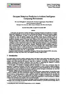
Figure 2.2: Lightswitch-2002 algorithm for the electric lighting and blinds as presented in [11]. The diagram to the right corresponds to the “set blinds” procedure.

2.1. STATE OF THE ART 17


18

- daylight independent (Di) - the user controls the lighting system independently of ambient daylight conditions, and two towards blinds: - blinds dynamic (Bd) - the user uses the blinds on a daily basis, - blinds static (Bs) - the user keeps the blinds permanently lowered with a slat angle of 75 ◦ . The electric lighting system and blind status are set (according to the algorithm shown in figure 2.2) at each 5 minute time step depending on the irradiance on the workplace (DAYSIM, a daylight simulation method developed by Reinhart and Walkenhorst [26], provides irradiance data every 5 minutes based on hourly averages entered as inputs), the presence of the simulated occupant (either measured or simulated with the model presented earlier) and on which of the 4 above behaviours (s)he adopts (it is supposed that each occupant will adopt one of the above behaviours and behave consistently over the whole simulation period). Control of blind position can be automated, in which case they are lowered if the irradiance on the workplace reaches the arbitrary threshold of 50W/m2 , then slanted to an angle of either 0 ◦ , 45 ◦ or 75 ◦ to block the direct sunlight from causing risks of glare; they are lifted or kept open otherwise. An occupant with behaviour Bd will close blinds in the same way under the same conditions but only open the blinds on arrival into the office. Finally occupants with behaviour Bs will leave the blinds in the closed position all year round. Lighting systems are switched ON either at arrival (by occupants of behaviour Di) or when the indoor illuminance level is too low. The probability that an occupant with behaviour Dd considers the indoor illuminance level to be too low is given either by a distribution proposed by Hunt [27] in the case of arrival into the office or after the status of the blind has been changed, or by another distribution proposed by Reinhart and Voss [28] in the case of intermediate switch ON (i.e. while the occupant is in the office). The lighting system is switched OFF only at departure; the probability of this event happening depends on whether the system is equipped with occupancy sensors or not (based on observations made in [29] and [28] that the latter systems are more often left ON by the occupant). Systems equipped with sensors and left ON will switch OFF after a specific number of time steps; systems not equipped with occupancy sensors will be switched OFF at the occupant’s departure with a probability Pclosing based on their likely duration of absence. Lightswitch-2002 is the most comprehensive model to date for the integration of occupant behaviour towards lighting appliances and blinds into dynamic building simulation tools. Yet it does suffer from clear limitations discussed by its author in [11]: - so far it is restricted to one- and two-person offices; - the author does not know how well the four types of behaviour proposed represent the true behaviour of people and, if they do, what proportion of occupants corresponds to each type of behaviour;


19

- the consideration that lighting systems are only turned OFF once a day and that blinds will only be opened once a day is restrictive and needs to be further investigated. Nevertheless, when applied to a case study the model predicted a 20% saving in energy for offices equipped with occupancy sensors, which agrees with field measurements.

2.1.3

Integration of occupant models

We have discussed within this chapter different ways of considering the effect of occupants on the energy consumed by buildings (for heating, cooling and ventilation) and within buildings (electricity consumption of appliances and lighting systems). These can be grouped into three categories: - those that consider occupant presence and behaviour in a statistical way, - those that combine occupant presence with occupant activity, - and finally those that consider occupant presence to be a necessary condition for occupant interaction with the building and simulate the two separately, considering the former to be an input to the latter. Diversity profiles are an example of the first method: a profile of hourly values ranging between 0 and 1 is chosen for a type of interaction (metabolic heat gains resulting from occupant presence, internal heat gains resulting from the use of office appliances, of lighting appliances, etc.) and then multiplied by the measured or estimated peak value of the variable of interest. The resulting profiles are then used as the input of internal heat gains to either a steady state or dynamic building energy simulation program. Yamaguchi et al. ([13] and [30]) are interested in choosing the optimal set-up of plant systems (mix of technologies, sizing and network design) that can cover the thermal and electrical needs of a city district. Its electrical load profile is composed of fixed schedules, for lighting systems and appliances used collectively, and the consumption profiles generated by the stochastic model of the occupant’s activity at her/his office desk. We believe that the amalgamation of occupant’s presence and activity actually weakens the model, therefore we are in favour of separating the two because occupant presence can be used as an input to any model of occupant behaviour (so that the results are directly reusable), but not all of these models require the different activities of the occupant in order to function correctly. The added information of activity can be useful but it comes with a cost: the more activities we wish to consider the more information we will need on the probability of the occupant exercising these activities and, in the case of Markov chains (the method proposed by Yamaguchi) on the probabilities of transition from one activity to another. The task of generating a model of occupant presence that is easy to calibrate and can be used as an input for any model of occupant behaviour of any type of building is already a great challenge. Once this challenge has been met, one could devote more effort to developing separate models of occupant behaviour using presence as an input.


20

This method was adopted by Bourgeois [31] in the development of his sub-hourly occupancy control (SHOCC) model, described by himself as being a “self-contained, whole-building energy simulation module that is concerned with all building occupant related events” [32]. SHOCC works as an independent module that handles all information related to the presence and behaviour of the occupants that are used as inputs to simulation tools such as ESP-r (the tool used for its development). SHOCC updates ESP-r only when necessary and with the needed information at the right time step of the tool’s algorithm, making it unnecessary for ESP-r itself to consider the occupants of the building. To do so it needs: - a database, with all the information related to the occupants and the objects they use, - a model of occupant presence (the model discussed in [31] is the one present in Lightswitch-2002), - and models of occupant behaviour (those discussed in [31] are Lightswitch-2002 and a simplified model simulating the use of a laptop). Bourgeois claims that any model of occupant presence and behaviour can in principle be used within SHOCC, and that SHOCC can communicate with almost any building simulation tool; its main asset is to provide a platform linking the former to the latter. Of course the crucial issue is to develop models that prove themselves capable of simulating occupant presence and the aspects of occupant behaviour that have an impact on the resource flows (e.g. energy demand) within a building.

2.2

Family of stochastic models integrated into SUNtool

We present here our own efforts in developing a set of stochastic models capable of integrating the impact of occupants on the building they occupy and with which they interact. This work was conducted as a part of the “project SUNtool”; the models were integrated within the modelling tool developed during the project.

2.2.1

SUNtool

Funded under the European Community’s 5th Framework Programme, Project SUNtool8 (for S ustainable U rban N eighbourhood modelling tool ) was a three year research project (from 2003 to 2005) that united 6 teams of collaborators from 6 different European countries (BDSP Partnership from London, England, the Czech Technical University of Prague, Electricité de France, IDEC S.A. from Athens, Greece, the Technical Research Centre of Finland and the LESO-PB of the EPFL this last team was composed of my colleague Nicolas Morel and myself) to develop a tool that can help designers to optimise the sustainability of urban neighbourhoods (see [33] and figure 2.3). The aim of project SUNtool was “to develop an integrated 8

Detailed information on SUNtool as well as a downloadable version of the software can be found at the website www.suntool.net.

Figure 2.3: Workflow stages in the use of SUNtool: 1. Choice of location; 2. Choice of iDefault set or replacement with values entered by the user; 3. Use of the 3D sketching tool to draw and attribute buildings; 4. and 5. Management of simulations; 6. Display of results.

2.2. FAMILY OF STOCHASTIC MODELS INTEGRATED INTO SUNTOOL 21

22


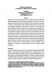
Figure 2.4: Structure of the SUNtool modelling tool and detail of the exchange of information between the models of the solver (see [34]). resource flow Modelling tool and associated Educational Tool to support sustainable urban planning - so that urban planners are equipped both with sustainable masterplanning guidance as well as a comprehensive software tool for quickly optimising the performance of the master-plan.”[35] The educational tool contains a set of guidelines and case studies to acquaint the user with the concept and technicalities of sustainable urban planning, as well as a tutorial for the use of the modelling tool. The latter is composed of (see figure 2.4): - a transient heat flow solver. This is the core of the modelling tool. It calculates the heat flowing in and out of each zone9 of each building with a time step of one hour. - an advanced radiation model that is run before the main simulation is carried out by the core solver and provides it with inputs of short- and long-wave radiation as well as daylight entering the building. 9 The thermal solver first splits the building vertically into zones of identical use (i.e. residential zones and offices zones). Each floor is then split into a “passive zone”, on its periphery, and a “non-passive” core zone. Within the stochastic models, we consider a zone to be a flat containing one household in the case of a residential building (or the residential zone of a mixed building), or an office (singly or multiply occupied) in the case of an office building.

Figure 2.5: Functionalities of the GUI.



24

- plant and equipment models for the local production of resources (heat and cold, electricity, recycled water and possibly bio-fuels). - and the stochastic occupant-related models we discuss in this thesis. A user-friendly graphical user interface (GUI - shown in figure 2.5) accompanies the user through the different steps of the simulation of the neighbourhood. The first step is to define its geographical location (loading the solver with the appropriate climate files and national data sets of default properties with which to attribute individual buildings). The buildings can be entered using a 3D sketching tool; the user can then attribute properties to each of these by adopting the proposed “iDefaults” (simply by defining their use and age - which themselves have default values) as shown in figure 2.6. These i ntelligent Default values are data sets corresponding to national statistics (e.g. of occupant-related parameters, construction guidelines, regulations) that were collected by the partners during the project and integrated within the tool’s database. By using these default attributes, or updates of them, for given buildings or parts of buildings, the SUNtool solver can simulate the whole or a fraction of the given neighbourhood for any period of time up to a year. The micro-climate models run independently of the solver in a pre-processing stage; so do the stochastic models of occupant presence and behaviour aside from the model of the window opening; the latter communicates with the solver during the processing stage, providing it with inputs as well as receiving inputs from it at each of its time steps (see figure 2.4). At the end of the simulation the GUI displays a table summarising key environmental performance indicators for the modelled master-plan as well as a series of standard graphs (see figure 2.7), enabling the user to assess the value of the scenario simulated (lay-out and choice of properties of buildings and plants). Hourly results of key variables may also be exported for further analysis using proprietary data analysis tools

2.2.2

Stochastic models of occupant presence and behaviour

This chapter has exposed the reasons why the integration of occupants’ interactions with buildings has become a necessity and how this has been done by fellow researchers. In addition, we have argued that: - White-box models are more flexible than black-box models and will therefore be easier to adapt to changes in occupants’ behaviour and in the objects they use. Their use should therefore be preferred as long as this is possible. - The presence of an occupant is a necessary condition for her/his interaction with a building. Occupant presence should be simulated separately and serve as an input to models of occupant behaviour. Developing an excellent model of occupant presence should be our first priority as the quality of its output will limit the quality of the outputs of occupant behaviour models. Based on the literature review and the above hypotheses we have identified the need for a set of 5 stochastic models (see figure 2.8) to simulate: - the presence of occupants within a zone,


Figure 2.6: SUNtool’s 3D sketching tool and attribution of the building’s properties. Design of a neighbourhood of buildings with the sketching tool and attribution of the use of each building.

CHAPTER 2. CONTEXT OF RESEARCH 26

Figure 2.7: Display of typical outputs of the SUNtool modelling tool.


Figure 2.8: Set of the stochastic models integrated into SUNtool. Fine arrows describe information delivered by one model to another, thick arrows represent information used directly as an output of the modelling tool. - their use of the appliances of that zone, - their use of windows of that zone’s facade, - their production of solid waste, - their use of the lighting system and blinds of the zone. The spatial resolution of these models, i.e. the “zone”, is an office room (occupied by one or more occupants) in the case of office buildings, or a flat inhabited by one household in the case of residential buildings (so far SUNtool only considers these two types of buildings). The temporal resolution varies from one stochastic model to the other. Presence The model of occupant presence simulates the state of presence (“absent” or “present”) of each occupant of the zone at each time step. Its output serves simultaneously as an input to the thermal solver by providing it with the total metabolic heat gains accumulated over the hourly time step and as an input to all the models of occupant behaviour. This implies that the model has to reproduce different characteristics of occupant presence; for example, the cumulated presence over a day or a week might be a level of detail sufficient for the thermal solver or the model of solid waste production, whereas the models of appliance and window use will need to have reliable information on the time of arrival and departure of the occupant into and out of the zone or the periods of intermediate absence. The temporal resolution of this

28


model should therefore be dictated by the finest resolution required by related models. Although any divisor of an hour could be used, we have opted for 15 minutes; our choice has also been conditioned by the resolution of the data used to calibrate the model. We have chosen to use the profile of probability of presence as its main input, as this is a standard input to building simulation tools and should be easily accessible to the user. Other inputs are parameters related to long periods of absence and a parameter we have chosen to represent the typical mobility of occupants. The model is discussed in great detail in chapter 3. Use of appliances The model of appliances is discussed in chapter 4. Appliances considered are household and offices appliances that consume electricity or water (hot and cold) or both. The output of the model will provide the thermal solver with the internal heat gains accumulated over the hourly time step due to appliance use and export to plant and equipment models profiles of electricity, water and hot water demand as well as the production of wastewater. This is useful for designing plant and storage capacities as well as the distribution network as these will have to cover all or a fraction of the neighbourhood’s needs in resources. We have opted for a behavioural model. Appliances are split into categories related to their dependence on occupant presence for their use; each category is then simulated differently. A temporal resolution of 15 minutes was chosen in the case of offices and 2 minutes in the case of residential zones due to the resolution of the data collected; although any time step could be used. The input to the model is data related to the appliances (e.g. type, number, peak and stand-by power demands), either entered by the user or given by the iDefaults, as well as the profile of presence generated by the model of occupant presence. As the model of appliance is considered to be independent of the thermal conditions in the building it can run before the thermal solver as a pre-process. Use of windows The model of window use is the only model that communicates bi-directionally with the thermal solver and therefore needs to run simultaneously with it. It simulates the exchange of air of the zone with the outside. Occupants choose to open and close windows based on the thermal and olfactory comfort they experience within the zone. Randomness results from changing climatic conditions, the changing number of people present within the zone and the level of tolerance each occupant has towards the coolness, the heat and the concentration of pollutants of the air within the zone. The model calculates the amount of air exchanged through the window over an hour and provides this to the thermal solver. From the solver, it receives the indoor air temperature for each hour. Since this can change drastically if a window is left open for one whole hour, we have integrated into the model a simplified thermal solver that calculates the indoor air temperature every 5 minutes thereby allowing for the simulation of window openings of such short lengths of time. Other inputs are the profiles of presence for the zone and data related to its glazing (and openable proportion) area. The model is discussed in greater detail in chapter 5.

2.2. FAMILY OF STOCHASTIC MODELS INTEGRATED INTO SUNTOOL 29 Production of solid waste This model, described in chapter 5, is a simple attempt to estimate the amount of solid waste produced per building and the fraction of it that could be reused within the neighbourhood (mainly as a bio-fuel). It is basically an empirical model and therefore strongly depends on the data available. The temporal resolution chosen is 1 week which more or less corresponds to the frequency of collection of household waste. The output gives the amount of solid waste produced per zone in a week and its separation into recyclable wastes (including organic waste, metal, paper and glass). Use of blinds and lighting systems The model for the use of blinds and lighting system by the occupant integrated within SUNtool does not figure within this thesis report. It is an adaptation, by Nicolas Morel, of the Lightswitch-2002 model proposed by Reinhart [25] discussed previously within this chapter. It provides the thermal solver with the internal heat gains due to the use of electrical lighting appliances as well as the position of blinds (which could be used in the future to calculate the solar heat gains let into the zone). Combined with the output of the appliance model, it also provides SUNtool with the electrical load profile of each zone of each building.

30


Chapter 3

Occupant presence 3.1

Introduction

Being present within the building is clearly a necessary condition for being able to interact with it. Occupant presence is therefore an input to all other models and the model for occupant presence will be central to the family of other stochastic models [36]. Furthermore, since humans emit heat and “pollutants” (such as water vapour, carbon dioxide, odours, etc.), their presence directly modifies the indoor environment. A model capable of reproducing patterns of presence of occupants in a building is therefore of paramount importance in simulating the behaviour of occupants within a building and their effects on the buildings’ demands for resources such as energy (in the form of heat, cold and electricity) or water as well as the production of waste (which may be later used to derive energy). We discussed in chapter 2 the use of diversity profiles for integrating metabolic heat gains resulting from occupant presence into simulation tools. The weakness of this method lies in the repetition of one, sometimes two, rarely three profiles (usually a “weekday” and a “weekend” profile, the latter sometimes being split into a “Saturday” and a “Sunday” profile) and the fact that the resulting profile represents the combined behaviour of all the occupants of a building. The latter simplification reduces the variety of patterns of occupancy particular to each person by replacing it with an averaged behaviour. The former simplification neglects the temporal variations, such as seasonal habits, differences in behaviour between weekdays (that appear in monitored data) and atypical behaviours (early departures from the zone, weeks of intense presence and of total absence, unpredicted presence on weekends in the case of office buildings - events that all appear in monitored data). An improvement on this approach is a simple stochastic model which is present within [11]. This introduces some randomness in the arrivals and departures of occupants into offices as we have seen earlier. While this represents a certain progress towards a realistic simulation of occupant presence the fact that the major portion of the profile is fixed (presence of 100% during most of the working hours, presence of 0% from 18:15 to 7:45, repetition of the same profile for all weekdays and the assumption that the zone is unoccupied during weekends) prevents the model from reproducing the variety both in behaviours and over time of occupant pres31

32

CHAPTER 3. OCCUPANT PRESENCE

ence. One important aspect of this restriction is the lack of periods of long absence (corresponding to business trips, leaves due to sickness, holidays, etc.) leading to an overestimation of the total yearly presence and associated energy consumption, as recognized by the authors. The appearance of occupants on weekends, their arrival before 7:45 and departure after 18:15 are phenomena that are common to the real world but are omitted by the model. Finally the absence of occupants outside of breaks is also an event that it fails to simulate. Wang et al. [12] attempted a clear move away from fixed profiles of presence. The daily presence of an occupant in a singly occupied office is modeled with a random arrival followed by alternating periods of intermediate absence and presence whose length is distributed exponentially. They propose a truly stochastic model for occupant presence. This is simple and elegant but it still fails to reproduce the complexity of real occupant presence. As the authors acknowledge themselves, periods of presence cannot be reproduced by an exponential distribution with a homogeneous coefficient, and times of arrival, of departure as well as absences during lunch breaks are not normally distributed. Like all its predecessors the model supposes that all weekdays are alike and that offices are always unoccupied during weekends. Periods of long absence are also neglected so that total presence is once again overestimated. The motivations behind the model proposed by Yamaguchi et al. [13] are very similar to ours. They want a model that can predict the heating, cooling and electricity loads of a commercial building. Part of this will result from occupant presence and activity and these are amalgamated into the four states an occupant can be in: absent, present but not using a computer, present and using one or two computers (for more details see chapter 2). In our work however we prefer to decouple occupant presence from any activity thereby ensuring that the output of the occupant model can be used by any model requiring occupant presence as an input. Furthermore it is not clear in their explanation of the model in [13] whether it is being used to simulate only one repeated day of occupant activity or each and every day of the year. In the latter case it is also unclear whether weekends are treated differently or whether periods of long absence are considered; we suppose that this is not the case. The calculation of an occupant schedule for only one day, if this is the case, would be restrictive as we have argued above and the lack of long periods of absence when simulating a whole year would likewise be erroneous as we shall explain below. The hypothesis that the duration of time an occupant spends in a given working state does not depend on time (i.e. the time of day) is one that Wang proved to be wrong in at least the case of presence. Dividing the state of presence into different states of working activity during presence will most probably not change that. Although their model could prove useful when only considering the use of PC’s, the hypothesis of time-independence shall cause difficulties when wanting to simulate less invariable activities such as the use of lighting appliances or activities performed in residential buildings for example. We propose in the following pages an alternative model for the simulation of occupant presence. By using a profile of probability of presence, rather than an adjusted fixed profile, as an input to a Markov chain we are able to produce intermediate periods of presence and absence distributed exponentially with a time-dependent coefficient as well as the fluctuations of arrivals, departures and typical breaks. A

3.2. MODEL DEVELOPMENT

33

failed attempt to validate an earlier version of the model highlighted the importance of periods of long absence and led to important amendments to the model. Twenty zones of an office building were monitored providing us with two years of data that was used for the calibration and validation of the model. The latter was based on the analysis of statistics of importance for the stochastic models of occupant behaviour that will use the results of the model of presence as their input. Although it was tested with data from an office building, this model, when given the corresponding inputs, is applicable to any type of building and any pattern of occupant presence.

3.2 3.2.1

Model development Aims

It is important to know what properties need to be reproduced by the model as they shall serve as a guideline for its development and as statistics to be checked during its validation. The model of occupancy is destined to deliver the metabolic heat gains and pollutants released by the occupants within the zone and to serve as an input for the use of windows, lighting appliances and other electrical and water appliances (see figure 3.1). To serve this purpose it needs to reproduce, in the most reliable way, properties of patterns of occupancy such as the first arrival and last departure of the occupant, the duration of the periods of intermediate presence and absence, as well as of long absence and the time of intermediate arrival for each and every occupant. Patterns of occupancy are so diverse and complex that we decided that the simplest way to develop a model capable of doing this was to build it from a priori hypotheses and check later whether the above properties are reproduced within reason.

3.2.2

Hypotheses

We are interested in simulating the presence of occupants within a specific “zone” of a building. This corresponds to the area occupied by a household in the case of residential buildings (typically a flat) and to a (single or multiple person) office in that of office buildings. We are not interested in simulating the movement of occupants from one zone to the other (a model for this has been proposed by [37]), but simply whether each occupant is present within the zone or not. The hypothesis of independence allows us to model in a simple way the patterns of presence of each occupant individually. The presence of occupants sharing the same zone can then be simulated by: 1. multiplying the obtained pattern by the total number of occupants (this case of collective behaviour would correspond to the occupancy of a meeting-room), 2. or by simulating each occupant separately and then adding the produced patterns of presence. We make the hypothesis that the probability of presence at a time step only depends on the state of presence at the previous time step. In other words the probability that an occupant is present now only depends on whether (s)he was


34

Occupancy [# of people]

ts

Resource consumption electricity and water

Lighting utilities [W and state of blinds]

n ta llu Po

Electrical / Water appliances [W / m3 of water]

Presence

Presence

Metabolic heat gains

Presence

Internal heat gains

Windows [m3 of exchanged air]

Ventilation

Figure 3.1: Outputs of the occupancy model and their direct and indirect impact on a building’s consumption of resources. present one time step ago and not on whether (s)he has been present over the past N time steps. Mathematically this statement corresponds to asserting the following property on the conditional probability: P (Xt+1 = i|Xt = j, Xt−1 = k, ..., Xt−N = l) = P (Xt+1 = i|Xt = j) =: Tij (t)

(3.1)

with Xt being the random variable “state of presence at time step t” and i, j, k and l taking on values 0 (absent) or 1 (present). This corresponds to considering the state of occupancy as a Markov chain with probabilities of transition Tij (t) (for more details on Markov Chains we direct the reader to [2]). The probability that an occupant should arrive at the office at 8:00 or at 22:00 are clearly not the same, therefore the values of Tij (t) need to be time dependent and we have the general case of an inhomogeneous Markov chain (with discrete states and discrete time steps).1 In order to determine the time dependence of these probabilities of transition we will need the following inputs to the model: the profile of probability of presence over a typical week and a parameter of mobility that gives an idea of how much people move in and out of the zone. 1

We will determine the initial state (at t0 =00:00 on January the 1st) of the time series as “present” for residential buildings and “absent” for office buildings.


3.2.3

35

Development

Based on our hypotheses we are looking for a model capable of generating a time series of zeros (absence) and ones (presence) that renders arrivals into and departures from the zone (typically going to work and coming from work for residential zones, arriving at work and leaving work for office zones) as well as alternating short periods of presence and absence in between. It should not simply reproduce the pattern given as an input (the profile of probability of presence and the parameter of mobility) but create a pattern that never repeats itself while reproducing the statistics of the real world it is simulating. To do this we have based the model on the inverse function method (IFM)2 that generates a time series of events from a given probability distribution function (PDF). Earlier we made the hypothesis that the value of occupancy at the next time step should only depend on the state we are in now and the probability of transition from this present state to either the same state (0 to 0; 1 to 1) or its opposite state (0 to 1; 1 to 0). These probabilities of transition T00 , T01 , T10 , T11 are therefore the PDF’s we need (in this case the values that the random variable can take are discrete). Only two of the four variables need to be known, let us say T01 and T11 , as T00 and T10 can be deduced from T00 + T01 = 1 and T10 + T11 = 1. As we have seen in previous models, the profile of probability of presence is a rather standard input for a simulation tool including occupancy and should be available to the user.3 Having this as an input provides us with a relationship for the probability P (t + 1) that the occupant is present at the time step t + 1: P (t + 1) = P (t) · T11 (t) + (1 − P (t)) · T01 (t)

(3.2)

From this we can deduce that : T11 (t) =

P (t) − 1 P (t + 1) · T01 (t) + P (t) P (t)

(3.3)

However, we still lack one piece of information to be able to determine uniquely the value of T01 and T11 at all times. This further input to the model should make sense to the user who will be entering it. Keeping this in mind we defined the “parameter of mobility” as the ratio between the probability of change of the state of presence over that of no change: μ(t) :=

T01 (t) + T10 (t) T00 (t) + T11 (t)

(3.4)

To simplify the inputs to the model we consider μ(t) to be constant and to assist the user of the model we will define numerical values to levels of “low”, “medium” and “high” mobility. It is important that these values be well adapted to the length 2

An explanation of the inverse function method and what we understand by “selecting” a number, or a value, given a probability density function are provided in Appendix A. 3 In the case of users unfamiliar with such inputs, default profiles corresponding to types of occupants will have to be made available.


36

of the time step used for the simulations.4 Given relationships (3.3) and (3.4) and the inputs P (t) and μ we should now have a complete profile of T01 (t) and T11 (t): T01 (t) = T11 (t) =

μ−1 · P (t) + P (t + 1) μ+1 P (t) − 1 μ − 1 P (t + 1) · · P (t) + P (t + 1) + P (t) μ+1 P (t)

(3.5) (3.6)

Unfortunately not quite. For certain values of P (t), P (t + 1) and constant μ, the condition 0 ≤ Tij (t) ≤ 1 can be violated. This typically happens when P (t) is far greater or smaller than P (t + 1). This situation corresponds to an almost deterministic change in behaviour, such as a regular time of first arrival into the zone, a regular lunch break or a regular time of last departure from the zone, rather than the random movement into and out of the zone expressed by a constant value of μ. In each of these cases the model would fail to reproduce such clear changes in occupancy when using the initial value of μ; to counter this the model temporarily replaces the value of μ, for that particular time step, by one that fulfills the above condition and is closest to the initial constant. For an initial fixed value of the state of presence at t0 we are now able to generate a time series of the presence of an occupant within a given zone. This first version of the model was calibrated with data of occupancy recorded in the offices of the LESO building (for more details on the building see [38]) and a preliminary validation was made by comparing the cumulated presence over a week resulting from the original data and the simulations done with the model (this can be seen in figure 3.2). The data contained a great variety of results ranging from weeks of total absence, corresponding to periods of leave due to sickness, work outside of the office or vacations, to weeks of high cumulated presence, corresponding to periods of overtime work and unusual presence over weekends. The model was only capable of producing a Gaussian-like distribution centered around the average of the empirical data. This showed that, although the Markov chain model works well at reproducing periods of short absence and presence during one day, it needs to be complemented in order for the model to generate long periods of absence. These have been included by adding to the algorithm the possibility to start, at random, a period of long absence at each time step.5 To generate them we need to know the probability of them happening and the parameters that determine the distribution of their duration; these shall be new inputs to the model. For the validation of this improved version of the model of occupant presence the periods of long absence (lasting more than one day but not corresponding to a weekend) were extracted from the empirical data and treated to give the necessary inputs to the model. The remaining data was used to calibrate the Markov chain. 4

We have already encountered a similar case of this in chapter 2 (see equation 2.4). In this particular situation, the probability of transiting from state i to state j in one hourly time step is Tij , while that of visiting state j starting from state i at least once within twelve 5 minute time n steps is Tij · 1 + 11 n=1 (1 − Tij ) . 5 This means that periods of vacation will be distributed randomly over the year rather than attributed to fixed days of the year.

Figure 3.2: Cumulated hourly presence (in hours - x axis; occurrences - y axis) of 115 weeks from various LESO offices (solid red line) compared to the results from the first version of the model (solid blue line).

3.2. MODEL DEVELOPMENT 37


38

Figure 3.3: Preprocessing stage: extraction from the inputs of the probability distributions needed for the inverse function method to be used in the processing stage.

3.2.4

Algorithm

The model was implemented as a MatLab script. The presence of each occupant in each zone was simulated independently based on the inputs related to that occupant. The profile of probability of presence and the parameter of mobility are used to determine the profile of T01 and T10 (see figure 3.3). The occupant is considered to be absent in the case of office buildings and present in that of residential buildings at t0 , i.e. 00:00 of the 1st of January. From then on the time series of presence is generated by using the IFM at each time step. Figure 3.4 shows how the algorithm works: given the probability of starting a period of long absence (derived from the number of long absences happening in a year, entered as an input) we first check whether the occupant starts a period of long absence or not by using the IFM, if so we determine the length of that absence given the distribution of the duration of periods of long absences (entered as an input) with the same method, during which period the occupant is considered to be absent. At her/his return, or if (s)he did not start a long period of absence, we find ourselves in the case of the Markov chain of “usual daily” changes in state of occupancy. The present state of occupancy will tell us which profile of probability of transition to choose between T01 and T10 ; the next state of presence is determined by the use of the IFM. By doing so we are capable of generating a time series of the state of presence of a particular occupant in a particular zone. The state of presence of each occupant of one zone and the states of occupancy of different zones being considered independent it is enough to repeat this algorithm as many times as the number of total occupants, respecting, of course, the inputs particular to each


Figure 3.4: Algorithm of the model (processing stage).

39


40 occupant simulated.

3.3 3.3.1

Results Data collection

The data needed for the calibration and validation of the model was collected from mid December 2001 to the beginning of January 2006 in 20 “zones” of the LESO-PB building at the EPFL each equipped with a movement sensor. Of these, ten zones were offices having seen their number of occupants vary over the period of monitoring and five zones had not been constantly used as offices (printer room, conference room, classroom and workshop). The remaining five zones which had been singly occupied offices over the whole period of data acquisition, were used for model calibration and validation. The people at the LESO work mainly on research, sometimes taking or giving courses. Occupants are very mobile often leaving their office to visit other zones of the same building, such as the workshop, the library or computer-room or offices of colleagues, or to leave the building. This may make the patterns of presence not particularly representative of an office building (and even less so of a residential building!). Nevertheless, this shall not weaken the validation of the model as it has been conceived to be independent of the characteristics of the occupants to be simulated. Indeed only the inputs to the model (profile of probability of presence, parameter of mobility, distribution of periods of long absence) are related to the simulated occupants; the model itself, given the right inputs, should be applicable to any type of building and any pattern of occupant presence.

3.3.2

Treating data for calibration

The acquired data needed to be processed before information for the calibration and validation of the model could be extracted. Problems either with the sensor, the bus used for the transfer of monitored data or with the server used to store the data caused gaps within the acquired data, reducing the amount of usable data to approximately 2 years and the longest period of uninterrupted data acquisition to approximately 6 months. Also the acquisition system only records changes of the variable to be acquired; in the case of occupancy this means that the time and date are recorded: 1. the first time the sensor notices motion in the office when it previously considered it to be empty - this corresponds to a switch to the state “occupied”, 2. when the sensor has not noticed any movement for 30 seconds in an office considered to be occupied - this corresponds to a switch to “vacant”. The sensor only recognizes two states of presence: occupied or vacant, and can therefore not distinguish whether the zone is multiply occupied or not. This however is not a problem, since the presence of guests in an office is dependent upon whether the owner of that office is present so that the owner-occupant presence is continuously accounted for. The first step in processing the raw data was to check which days of acquisition had suffered from the technical problems stated above and

3.3. RESULTS

41

only conserving those that are completely intact. This data was then cleaned of all periods of absence lasting less than 2 minutes (this usually corresponds to a sensor that stops recording the presence of an occupant because (s)he is too still for her/his movement to be noticed). We then constructed a time series of the data with a 15 minute time step by summing over each 15 minute interval the duration of periods of presence and of absence and allocating to that interval the state with the longest total duration. The treated data could then be used for the extraction of information first of all to deduce the inputs necessary to calibrate the model, then to have reference data for its validation. The first step was to check the length of both periods of presence and of absence. The periods of absence were then divided into periods of “short” absence (less than 24 hours), of absence that could be related to weekends and periods of “long” absence (greater than 24 hours but not taking place over a weekend).6 Periods of long absence were studied to deduce the distribution of their duration and the average number of their occurrences in one year, which will both serve as inputs to the model. The long absences were removed from the time series and the remaining data was used to provide information on the day-to-day occupancy such as the profile of probability of presence and the profiles of probability of transition T01 and T10 . A profile of the parameter of mobility was deduced from the profile of T01 and T10 by using equation (3.4). The average of the positive values of the profile is used as input to the model.

3.3.3

Validation

The occupancy model has been developed to simulate the time an occupant spends in a particular zone but above all to produce a time series of presence that will serve as an input for models capable of simulating the occupant’s behaviour. Each of these models may have different expectations of the occupancy model’s output; while a model for the opening of windows needs reliable information on the time of arrival of the occupant, a model for the use of household appliances will need to know how long the occupant’s periods of presence will last. In order to estimate the success of the model we listed the statistics that should cover each of these expectations: - the effective total amount of presence will be given by the “cumulated presence per day” and “cumulated presence per week”, - the “first arrival” into the zone and the “last departure” from the zone of each day of presence; the difference between these two corresponds to the duration of “daily presence” (in contrast to the duration of effective presence mentioned above), - the duration of “periods of intermediate presence” and of “periods of intermediate absence”, 6

Most intervals of acquired data are relatively short due to interruptions during data acquisition (intervals range from 2 days to 6 months with the average duration being 2-3 weeks). This of course limits the sample of periods of long absence available. It may also shorten periods of absence that could have lasted longer.

CHAPTER 3. OCCUPANT PRESENCE 42

0.7 0.6 0.5 0.4 0.3 0.2 0.1 0

0.5 0.4 0.3 0.2 0.1 0

0

0

96

96

192

192

384

Profile of probability of presence

288

Profile of parameter of mobility

288 384 Quarters of an hour (96 per day)

480

480

576

576

672

672

700

700

Figure 3.5: Comparison, between the monitored data (solid blue line) and the simulated time series (dotted red line), of the profiles of probability of presence (above) and of the parameter of mobility (below) for office no 3.

Probability

3.3. RESULTS

43

- the “number of changes” of the state of presence during the same day. We then compared the distributions of those statistics deduced from the measured data and from simulated data produced by the model. For each of the offices of the LESO building we produced a 5 year time series based on its calibrated inputs. From these time series we calculated the profile of probability of presence, the profiles of probabilities of transition T01 and T10 and the profile of the corresponding parameter of mobility as well as the distribution of the duration of long absences, in order to make sure that the model’s output is still consistent with its inputs. While the profiles of probability of presence compare very well, the simulated values of the parameter of mobility are clearly below those entered (see figure 3.5). This might be due to its relatively frequent recalculation (discussed in section 3.2.3) that could limit its impact. The time series used to calibrate the model and those resulting from the simulations were then processed to produce the distributions of the statistics of interest for comparison.

3.3.4

Discussion of results

We discuss here the results from 4 of the 5 “singly occupied” offices.7 The simulation of “multiply-occupied” offices shall nevertheless not be a problem for the future use of the model as the user will enter inputs for each occupant and each occupant will be simulated independently (unless a dependent behaviour is required, such as for a meeting room, in which case a single profile may be used). The green solid lines correspond to data from the monitored offices, the red dotted lines are the results from the simulations. We have shown both the PDF and the CDF of the statistics. For comparison we have added to the CDF’s the histogram(s) equivalent to a standard deterministic representation of occupant presence used in dynamic thermal simulation programs of buildings: 100% presence on weekdays from 8:00 to 12:00 and from 14:00 to 18:00. The results from the monitored data provide us with a valuable insight into what the statistics really look like and in understanding the influence of occupants on the building. We will now discuss the different categories of statistics and observe how well the model reproduces what happens in reality. Arrivals into and departures from the zone The first category of interest is that of the first arrival of the occupant into the zone and her/his last departure from the zone (shown in figures 3.6 and 3.7). The difference between the two, the “daily presence” (shown in figure 3.8), gives us an idea of how long the occupant could have interacted with the zone, although (s)he might not have always been present during that interval. The behaviour of occupants is usually very different at their first arrival and last departure than during any intermediate arrivals and departures. The first arrival of the occupant usually corresponds to the setting by the occupant of her/his environment to her/his favourite configuration, for example the setting of the state of the blinds, the state of 7

Although all five offices produced similar results, we show only four of them for aesthetical reasons.


Time of first arrival − office no.1

96

96

96

0

0.5

1

0

0.1

0.2

0.25

0

0.5

1

0

0.1

0.2

32 48 Quarters of an hour



96

0.25

0

0

0.2 0.1

0

1

0.5

0

0.2

0.25

0.1 0

1

0.5

0

0

Time of first arrival − office no.2


96

96

96


96

0

0


32 48 Quarters of an hour Time of first arrival − office no.4

0

Figure 3.6: Comparison, between the monitored data (green solid line) and the simulated time series (dotted red line), of the PDFs and CDFs of the time of “first arrival” into the zone for four private offices. The blue histograms correspond to the repeated use of a standard fixed profile.

0

32 48 Quarters of an hour Time of first arrival − office no.3

0.25

0

Pdf Cdf Pdf Cdf

Pdf Cdf Pdf Cdf

Pdf

Cdf

Pdf

0

0.5

1

0

0.05

0.1

0.15

0

0.5

1

0

0.05

0.1

0

0

0

0

72

48 Quarters of an hour


72

72

48 72 Quarters of an hour Time of last departure − office no.3


Time of last departure − office no.1

96

96

96

96

0

0.5

1

0

0.05

0.1

0.15

0

0.5

1

0

0.05

0.1

0.15

0

0

0

0

72



72

72

48 72 Quarters of an hour Time of last departure − office no.4


Time of last departure − office no.2

96

96

96

96

Figure 3.7: Comparison, between the monitored data (green solid line) and the simulated time series (dotted red line), of the PDFs and CDFs of the time of “last departure” from the zone for four private offices. The blue histograms correspond to the repeated use of a standard fixed profile.

Cdf

Pdf Cdf Pdf Cdf

0.15

3.3. RESULTS 45


0.2 0.15 0.1 0.05 0

1

0.5

0

0.2 0.15 0.1 0.05 0

1

0.5

0

0

0

0

Daily presence − office no.1


40 48 Quarters of an hour Daily presence − office no.3



96

96

96

96

0.2 0.15 0.1 0.05 0

1

0.5

0

0.2

0.1

0.15

0.05 0

1

0.5

0

0

0

0



40 48 Quarters of an hour Daily presence − office no.4


96

96

96

96

Daily presence − office no.2

0

Figure 3.8: Comparison, between the monitored data (green solid line) and the simulated time series (dotted red line), of the PDFs and CDFs of the “daily presence” within the zone for four private offices. The blue histograms correspond to the repeated use of a standard fixed profile.

0

Pdf Cdf Pdf Cdf

Pdf Cdf Pdf Cdf

3.3. RESULTS

47

the lights and appliances, the set-point of the heating system or the opening status of windows. These might often stay unchanged until the last departure, during which the occupant returns the zone to its unoccupied state (with, for example, lights and appliances being switched off, windows closed, etc), knowing (s)he will not be back until the next day or beyond. Although most values of arrival and departure correspond approximately to values one would expect (arrival around 8:00 ± 1 hour - corresponding to 32±4 quarters of an hour, departure around 18:00 ± 1 hour - corresponding to 72 ± 4 quarters of an hour) and that are adopted by other models of occupancy, the figures show that the times of arrival and of departure are particular to the occupant and that these times can depend on the day of the week simulated, explaining the lesser peaks. Values might be off by a time step or two (15 to 30 minutes) and the peaks from the original data might be spread out a little but the model captures quite well the different characteristics, recognising the main peak while also reproducing the later arrivals, earlier and later departures as well as the days of longer or shorter daily presence. It should be pointed out that the occasional very early arrivals that appear in the simulations are the result of the model reproducing the non-zero probability of the occupant being present overnight that can be seen in the profile of probability of presence entered as input (figure 3.5). One can also notice in figure 3.8 the stochastic nature of the model: while some occupants will depart exactly ten hours after a first arrival that might fluctuate around an average (offices 1, 2 and 4), the simulated occupant might arrive and leave a bit earlier or later without the two being strongly correlated (just like the behaviour of the occupant of office no.3). Periods of intermediate presence and absence Figures 3.9 and 3.10 show the distribution of periods of presence and of short absence (less than 24 hours). So far the models that have tried to reproduce periods of intermediate presence and absence 8 have done so by assuming their duration is distributed exponentially and is independent of time. Standard profiles of occupancy propose the histograms shown with the CDFs; they correspond to 2 periods of 4 hours of presence separated by a two hour lunch break and the fourteen hours of absence between the last departure (at 18:00) of one day and the first arrival (at 8:00) of the next. The periods of short absence simulated by the model can be split into periods of such absence between workdays (the lower peak at the right of the figure) and periods of intermediate absence (to the left and smaller than, let us say, 48 quarters of an hour). Periods of very short presence and absence (1530 minutes) are clearly underestimated in the case of absence and only slightly in that of presence. Nevertheless the model confirms that presence does not follow an exponential distribution and that each occupant has her/his own behaviour, which the model picks up rather well. The lack of very short periods favours the occurrence of longer periods; a confirmation of this can be seen in the distributions of the number of changes per day of figure 3.11. These appear in pairs as none of the occupants ever stayed present overnight; each arrival is therefore followed by a departure. 8

Wang had some success in the case of periods of absence, while Yamaguchi has, to our knowledge, not published any validation of their model.


0.3 0.2 0.1 0

1

0.5

0

0.3 0.2 0.1 0

1

0.5

0

0

0

0

8

8

8

8


72

Periods of short absence − office no.1

24



72

72

24 48 56 72 Quarters of an hour Periods of short absence − office no.3

24

24

96

96

96

96

0.3 0.2 0.1 0

1

0.5

0

0.3 0.2 0.1 0

1

0.5

0

Periods of short absence − office no.2

96

72


24

96

8

72

96

0


72

96

24


8

8

24

0

0

8

24 48 56 72 Quarters of an hour Periods of short absence − office no.4

0

Figure 3.9: Comparison, between the monitored data (green solid line) and the simulated time series (dotted red line), of the PDFs and CDFs of “periods of short absence” for four private offices. The blue histograms correspond to the repeated use of a standard fixed profile.

0

Pdf Cdf Pdf Cdf

Pdf Cdf Pdf Cdf

Pdf

Cdf

Pdf

0

0.5

1

0

0.1

0.2

0.25

0

0.5

1

0

0.1

0.2

0

0

0

0

16

16

16

16


72

24

24



72

72

48 72 Quarters of an hour Periods of presence − office no.3

24

24

Periods of presence − office no.1

96

96

96

96

0

0.5

1

0

0.1

0.2

0.25

0

0.5

1

0

0.1

0.2

0.25

0

0

0

0

16

16

16

16


72

24

24



72

72

48 72 Quarters of an hour Periods of presence − office no.4

24

24

Periods of presence − office no.2

96

96

96

96

Figure 3.10: Comparison, between the monitored data (green solid line) and the simulated time series (dotted red line), of the PDFs and CDFs of “periods of presence” for four private offices. The blue histograms correspond to the repeated use of a standard fixed profile.

Cdf

Pdf Cdf Pdf Cdf

0.25

3.3. RESULTS 49


0.5 0.4 0.3 0.2 0.1 0

1

0.5

0

0.5 0.4 0.3 0.2 0.1 0

1

0.5

0

0

0

0

2

6

8 10 12 Number of changes

14

16

Number of changes in a day − office no.1

4

4

4

6

6



14

14

16

16

18

18

18

2 4 6 8 10 12 14 16 18 Number of changes Number of changes in a day − office no.3

2

2

20

20

20

20

0.5 0.4 0.3 0.2 0.1 0

1

0.5

0

0.5 0.4 0.3 0.2 0.1 0

1

0.5

0

20

20

Number of changes in a day − office no.2

18

20

20

16

18

18

14

16

16


14

2 4 6 8 10 12 14 16 18 Number of changes Number of changes in a day − office no.4

2

6


14

0

4

6


0

2

4

6

0

2

4

0

Figure 3.11: Comparison, between the monitored data (green solid line) and the simulated time series (dotted red line), of the PDFs and CDFs of the number of changes for four private offices. The blue histograms correspond to the repeated use of a standard fixed profile.

0

Pdf Cdf Pdf Cdf

Pdf Cdf Pdf Cdf

3.3. RESULTS

51

One can so far recognise that the model suffers from two flaws: 1. it underestimates the number of days of total absence, 2. it underestimates the number of changes by approximately one pair, suggesting less intermediate periods of absence and presence than seem to take place. This last discrepancy is probably linked to the drop in value of the parameter of mobility mentioned earlier; and, as occupants move less than in reality but their daily presence is realistically reproduced, longer periods of intermediate presence and absence will be slightly favoured as we have observed. Effective time spent in the zone So far we have discussed : 1. the times of arrival and departure of the occupant, stressing that these are the instants of a day when the occupant is most likely to interact with her/his environment (as observed for example by [9]), as well as the daily presence that gives an idea of how long the occupant will actively (when present) or passively (when temporarily absent) interact with the zone, 2. the number of changes of the state of occupancy and the durations of periods of presence and short absence that take place during one day, that give an idea of how often the occupant might interact with her/his surroundings at intermediate arrivals and departures. What we need to know now is how much time the occupant effectively spends in the zone during a day, a week or the whole year. This will govern what heat gains and pollutants each occupant will emit as well as how much total time the occupant has to affect her/his zone of occupancy. This can be deduced from the presence cumulated (i.e. total number of 15 minute time steps) over one day or over a whole week. Figure 3.12 shows the total number of quarter hours of presence during a whole week. As we can see from the monitored data, although the occupants’ duration of daily presence is typically greater than 12 hours (48 quarters of an hour per week), her/his effective cumulated presence over one week averages to around 24 hours. This is explained by the great movement of occupants and the work time they spend outside of their office. It can also be explained by days of total absence from the zone that called for the revision of the model we mentioned earlier. By adding periods of prolonged absence we have been able to adapt our model to weeks of total absence and weeks of overtime giving us a similar spread distribution as with the collected data. A chi-squared test with α = 0.95 confirms that both histograms could be the result of the same distribution for these four offices. Even though the addition of periods of long absence to the model has drastically improved its performance we still seem to underestimate the number of days of complete absence. This can be seen from the value of the CDF at 0 quarters of an hour in figure 3.13, that teaches us that approximately 35 to 40% of days include no period of presence (2 days of absence per week, such as a weekend, would correspond


Pdf Pdf

0.05

0.025

0

1

0.5

0

0.05

0.025

0

1

0.5

0

0

0

0

80 120 160 Quarters of an hour

200

240

Cumulated presence over a whole week − office no.1

40



200

200

240

240

40 80 120 160 200 240 Quarters of an hour Cumulated presence over a whole week − office no.3

40

40

Pdf Pdf

0.05

0.025

0

1

0.5

0

0.05

0.025

0

1

0.5

0

0


200

240

Cumulated presence over a whole week − office no.2

40

40



200

200

240

240

0

0

40

40 80 120 160 200 240 Quarters of an hour Cumulated presence over a whole week − office no.4

0

Figure 3.12: Comparison, between the monitored data (green solid line) and the simulated time series (dotted red line), of the PDFs and CDFs of the “cumulated presence” over one full week for four private offices. The blue histograms correspond to the repeated use of a standard fixed profile.

0

Cdf Cdf

Cdf Cdf

0

0.025

0.05

0

0.2

0.4

0.6

0.8

1

0

0.1

0.2

0.3

0

0

0




96

96

96

Pdf 0.05

0

0.2

0.4

0.6

0.8

1

0

0.1

0.2

0.3

0.4

0

0.025

Cdf

Pdf

Cdf

0

0

0




Pdf

Pdf

0.05

0

0.2

0.4

0.6

0.8

1

0

0.1

0.2

0.3

0.4

0

0

0

0




Cumulated presence over a day office no.3 0.5

0.025

Cdf

0.4

Pdf

0

0.025

0.05

0

0.2

0.4

0.6

0.8

1

0

0.1

0.2

0.3

0.4

0

0

0





Figure 3.13: Comparison, between the monitored data (green solid line) and the simulated time series (dotted red line), of the PDFs and CDFs of the “cumulated presence” over one day for four private offices. The blue histograms correspond to the repeated use of a standard fixed profile. The bottom figure corresponds to the same PDF as above without a value of cumulated presence equal to zero.

Pdf

Pdf Cdf


Pdf


3.3. RESULTS 53


54

to 28.5%) while the model only predicts an absence of 23 to 28%. The top part of figure 3.13 shows the whole PDF of this distribution. By subtracting the bin of zero presence we get an idea of what the distribution of cumulated presence looks like for days when the occupant appears for at least 15 minutes (see bottom line of plots in figure 3.13). This shows us how well the model reproduces the statistic and how it covers very closely the whole span of the distribution.

3.4

Discussion

To fully grasp the contribution of the model of presence it is important to compare it with models already available. Those recently developed by Wang [12] and Yamaguchi [13] are the first capable of simulating, in a reasonably realistic way, the periods of presence and absence between an occupant’s arrival and departure from an office. However they are based on the fact that the duration of periods of presence is time-independent and periods of long absence are neglected. Both Wang’s analysis and the validation of our model (see figure 3.10) have shown that the former hypothesis is wrong whereas the validation of the first version of the model highlighted how important it is to consider periods of long absence when generating a time series of occupant presence. All other methods used to model occupant presence can be summarised by the repetition of a standard or averaged fixed profile, with, in the best of cases, the spreading of times of arrival and departure using a Gaussian distribution in order to avoid strong peaks [11]. The results above have shown that our model, while having simple inputs, is capable of producing a non-repeating time series of any length, including essential periods of long absence and otherwise reasonable movements to and from the zone resulting in an excellent estimate of the total time an occupant really spends within the zone simulated. It is true that the model underestimates the amount of days of total absence as well as the amplitude of real movement into and out of the offices. The former could be due to an underestimation of the number or duration of periods of long absence9 and/or to the overestimation of presence during weekends.10 The latter is probably due to the recalculation of the parameter of mobility. These two aspects need to be better understood and improved. Nevertheless the model has proven itself capable of simultaneously: - reproducing periods of absence, - picking up the trends of periods of presence that cannot be simply modeled by an exponential distribution, - smoothing the peaks of times of arrival and departure, 9

The probability that the Markov chain alone might produce a work day of complete absence is extremely small as it will try at each time step to direct the simulated profile of occupant presence towards the profile of probability of presence it is given as an input. 10 The profile of probability of presence given for Saturday and Sunday (see top plot of figure 3.5) typically corresponds to rare periods of continuous presence that, if the parameter of mobility is kept the same for weekdays and weekends, the Markov Chain will simulate as occasional ultra-short periods of presence.

3.5. CONCLUSION

55

- while also considering days of atypical presence or of total absence. Although the benefits of the model will become apparent in terms of numbers only once it is coupled to models of occupant behaviour, one can already assert from the distributions shown in figures 3.5 to 3.13 that: - (figure 3.5) people working during weekends will need power and maybe heating or cooling that will be predicted neither by the standard model nor by Wang’s model, but will be by our model. - (figure 3.6) Likewise, arrival earlier than that predicted by other models will correspond to extra-lighting time during the darkest days of the year, just as later arrival can correspond to saved lighting, - (figure 3.7) early departure could correspond to saved hours of lighting, - (fig. 3.9 and 3.10) there is potential for saving electricity by implementing a smart switch-off option for appliances and lights left on when occupants are not present during periods of intermediate absence. - The clear difference between figures 3.8 and 3.13 shows that, although occupants might be “at work” approximately ten hours a day, they only spend about half that time in their office. This corresponds to a ¨decrease of 50% of the predicted metabolic heat gains (within that zone) as well as a potential decrease in electricity consumption linked to the non-use of lights and appliances.

3.5

Conclusion

While there is still room for its improvement the model already produces a realistic picture of occupant presence within zones of a building, the basis for related models of occupant interactions with their environment. It has been conceived to be capable of simulating any pattern of occupancy of any type of building when given the corresponding inputs. This general nature of the model has allowed us to validate it with data from an office building and to still claim that it will be useful for the simulation of any other type of building, in particular residential buildings. The outcome of the validation shown here emphasizes the progress this model represents compared to the standard procedures used today and even the latest model recently proposed. Indeed, the model, although relatively simple, has proven itself capable of reproducing important characteristics of occupant presence such as the times of first arrival and of last departure, typical long absences and the effective time of presence of the occupant within the zone of simulation while using only a small set of simple inputs. It produces a time series of the state of presence that includes the typical randomness of human behaviour: each person arrives into and departs from the zone they occupy at different times; people tend to enter and leave the zone several times during periods of occupancy, reducing the amount of total time spent in the zone and increasing the number of departures from and arrivals into the zone; people may be absent from the zone during long periods of time.

56


This gives a more realistic picture of the time the occupant spends in the zone and how often (s)he might interact with her/his indoor environment; it also avoids the unnatural peaks that arise from repeating the same pattern for each occupant.

3.5.1

Possibilities of improvement

The data available for the calibration of the model was very detailed. As future (nonexpert) users of model will not have the possibility to enter such detailed inputs an effort should be made in simplifying the inputs, replacing quarter-hourly profiles of presence by hourly profiles and empirical distributions of the duration of long absence by theoretical ones whose parameters would be entered by the user. This simplification of the inputs to the model will have an impact on its results and the extent of that impact needs to be studied. The appearance of long periods of absence and the parameter responsible for the amount of movement in and out of the zone are both represented simply by a constant. These two inputs have a deep impact on the model; the dependence of its results on the value they take should be analyzed in order to assess the robustness of the model and to offer the user with reasonable inputs. While values of the average number of long absences are easily interpretable, the parameter of mobility μ is new and deserves some further study. As we have seen μ has to adapt to the length of the time series used for the simulations and some research should be devoted to creating tables of values that correspond to what one would expect from the labels “low”, “medium” and “high”.

Chapter 4

Appliance Use 4.1 4.1.1

Introduction Motivation

The aim of almost every building is to serve as a sheltered locus for human activities. Its consumption of resources can be split into those used by the HVAC and lighting systems to ensure a comfortable indoor environment to its occupants, and those used by the occupants themselves while tending to their activities. As we have discussed in chapter 2, the use of appliances to execute these activities has a double effect: - it is an important source of consumption of electricity and of hot and cold water by the building, - it is an indirect source of casual heat gains to the zones of the building that will need to be taken account of by the thermal solver used to simulate demand in heating and cooling of the building. Just as the “waste” heat given off by appliances can be at times beneficial in reducing energy consumption, so the re-usable wastewater (so-called “grey water”) can be recovered for various needs and thereby reduce the building’s consumption of potable water. The use of appliances within a zone (residential or office zone as treated here) can vary greatly from one example to the other. Baker [39] observed this in the case of electricity consumption per square meter of a sample of offices, while Eggimann [40] did the same for electricity and hot water consumption among the flats of a same residential building. The consumption resulting from appliance use indeed depends on the occupants using them, but in different ways. The types and number of appliances installed within the zone are an important factor often depending on the use of the zone, the number of people sharing the zone, and sometimes (but not necessarily) the “status” of the occupants (within society or within the hierarchy of their company). For appliances to be used by occupants these need to be present; people often present at home (e.g. housewives or househusbands and elderly people) will be more active consumers than those mainly absent. Finally the behaviour of occupants towards the appliances they use (switching them OFF or not at departure, 57

CHAPTER 4. APPLIANCE USE

58

using various appliances at once, their behaviour towards stand-by) will play an essential part in determining both annual consumptions and load profiles. Two main fields of research are interested in reproducing realistic time series of appliance use: building physics, to reliably model internal heat gains for HVAC and passive system design, and energy supply technologies (in particular low-voltage electricity networks), to assess the size and timing of peaks and related risks. As decentralised energy production is integrated into buildings and coupled to existing networks (in the form of grid-connected PV panels or small networks of CHP) researchers of both fields now need to model load profiles (i.e. power consumption profiles) with ever finer granularity and precision. Questions will arise such as: What is the optimum sizing of a local power plant and the network of clients it can reach? How many local power plants can a low-voltage grid bear before technical problems appear or demand and supply are no longer possible to coordinate? How efficient can demand side management be in shaving peaks and ensuring supply? How can we reliably calculate the cost of energy as a function of time? The answers to these questions will have a considerable impact on future urban energy scenarios.

4.1.2

State of art

Both fields of research (building physics and energy supply technologies) have their own tools for modeling the use of electrical appliances. Building physicists have mainly been interested in knowing how much heat given off by appliances will serve as casual heat gains to the zone during the heating season and what heat will need to be evacuated by cooling systems in the cooling season. Predictions of annual electricity consumption will also figure in building performance simulation tools as national norms (such as the Swiss norm SIA 380/4 proposed by the SIA, i.e. Swiss Society of Engineers and Architects [41]) fix upper limits for the consumption of electricity per square meter of building to be built or refurbished. The methods used for the consideration of appliances depend on whether the tool used to estimate the performance of the building of interest is dynamic or not. Non-dynamic (steadystate) tools will make predictions of monthly or yearly energy needs. As inputs they will typically use: - space-related parameters, such as the number of occupants per square meter, installed power per square meter of lighting appliances or of electrical appliances in general; - these may be combined with time-related parameters, such as the daily use of hot water per person per day, the number of hours spent within the zone per person and per day. The latest guide proposed by the SIA [8]) provides specialists with the values to be used for 44 different types of uses of the spaces simulated. The diversity profiles, discussed in chapter 2, are a more advanced and commonly used method for both dynamic or steady-state simulation tools to represent the heat gains induced by occupants’ presence and behaviour. They provide a value between 0 and 1 for each time step of a typical day for different source of heat gains.

4.1. INTRODUCTION

59

Typically one profile will represent occupant presence; it is multiplied by the total number of people occupying the building when integrated into the simulation tool. Other profiles correspond to the use of different types of appliances (lighting, office appliances, etc.); the values of the profile are then multiplied by the installed power of the type of appliances. Diversity profiles represent typical behaviours usually linked to the use of the building (residential, office work, other types of work) and the types of occupant (elderly people, families, single occupants, etc). An extensive report on the compilation of such profiles (used by the American simulation tools DOE-2, BLAST and EnergyPlus) has been produced by Abushakra [7]. Instead of the typical average profiles (occasionally supplemented by their standard deviation) the authors provide for each time step the 10th , 25th , 50th , 75th and 90th percentiles of the parameter of interest. They suggest the use of the 50th percentile for the calculation of the needs in heating and that of the 90th percentile for the sizing of cooling units. The 10th percentile gives a good idea of the base load of a building; this can be of value for assessing constant casual heat gains as well as valuable information for the sizing of renewable energy systems (as these will at least want to cover the base load). These profiles are compiled by collecting hourly total and appliancerelated consumption data of a maximum amount from buildings of different types (building use and types of occupants), treating the data to make it independent of variations over the year, normalising the values by dividing them by the peak power value of the building over the whole year of measured consumption, separating the days into “weekday” and “weekend” categories and then deducing, for each of the categories, the distributions for each hour of the day. The percentile diversity profiles are produced with the percentiles of the distributions of each hour. When using a dynamic simulation tool, the users can choose the weekday and weekend profiles corresponding to the building and occupants of interest, choose the parameters (occupant presence, lighting, office appliances, etc.) and percentiles they are interested in, multiply them by the peak values (total number of people, installed power) and enter them as inputs to the solver.1 As usual the limitations of such methods are the averaging of the variety of behaviours and of their variation with time. They provide a coarse estimation of internal heat gains, but the percentiles proposed by Abushakra do give valuable indications of how values cumulated over all the occupants of a building and over all the days of a whole year might vary. But if one is interested in a resolution finer than that of the building and the two day types provided, or in the elements that compose each type of diversity profile then these methods become less helpful. This is typically the case when trying to assess the demand in electricity of a building or a set of buildings, in what is called Demand Side Management (DSM). Traditionally the priority in the field of energy management has been to understand (and sometimes influence) the use of electricity in order to maximise benefits. In liberalised electricity markets distributors will buy from different energy producers at the lowest possible cost while securing a provision of electricity to their clients at fixed rates. The price of electricity will essentially depend on the type of plant 1

In the case of the simulation tool ESP-r convective, radiative as well as latent heat gains are considered separately and all heat gains of a type are cumulated to form one sensible casual heat gain profile.


60

producing it and how far in advance it is bought: for example nuclear power plants, that have no flexibility in their production, generating an almost constant amount of power all year round, will be a source of cheap electricity to cover the base load within demand. Hydro-power plants can provide electricity almost instantaneously and will be used as a last minute resort to cover unexpected peaks. The electricity market operates on a 30 minute basis and last minute buys are the most costly; an accurate prediction of demand is therefore essential in securing profits.2 This is so far the main motivation for research in DSM.3 It is accomplished by collecting data on the various electricity consumers (typically in national load profile studies), developing methods to model load profiles at different levels of cumulated consumption and developing strategies to reduce peaks or procedures to minimise the effects of blackouts. In chapter 2 we have discussed in detail two state-of-the-art models from this field developed by McQueen [18] and Paatero [19]. While McQueen’s model has proven itself useful for the immediate estimation of the maximum demand of a low-voltage network, as a “black-box model” it is intimately linked to the data used to develop it. Changes in the behaviour of occupants and in the ownership and consumption of appliances (new energy-efficient appliances replacing older ones, leaps in generations of appliances such as the switch from PC’s to laptops, cathode ray tube (CRT) monitors to liquid crystal display (LCD) monitors, the disappearance of radios in favour of radio on the internet) cannot be implemented within his model because they are not considered to start with. New measurements would have to be made regularly to adapt to these changes. Because McQueen’s model does not distinguish the different appliances that play a role in the total consumption it is not able to simulate the casual heat gains of appliances whose energy consumption is not totally given off to the zone (such as dishwashers or washing-machines). Nor does it allow us to identify the electricity consumption linked to lighting appliances and therefore predict the energy that can be saved by adopting better control strategies or lighting systems. In addition to predicting the maximum load of a network, DSM may also help intervene in the electricity consumption of clients to shave the expensive peaks: this can be done by introducing time dependent tariffs or by prioritising the end-use of electricity and implementing strategies switching off appliances of lesser importance at specific times with the accord of clients. This requires a method that can split the end use of electricity consumption into that of different appliances, the so-called “bottom-up” approach that was adopted by Paatero. The strength of his model lies in the statistical method used to populate the building with appliances, and in the definition of the probability of switch ON which was used to start the cycle of use of appliances. However these are the only aspects of randomness included in the model, as appliances switched ON always function with the same constant power for 2

Nationalised electricity markets face similar issues as the producer-distributor monopoly wants to be sure he can cover demand while minimising an over-production that will not be paid for nor be useful. 3 As half the world’s population is not connected to a grid and extending existing networks will prove to be extremely expensive providing these people with electricity will involve the development of islanded scenarios of limited supply and also require the application of DSM.

4.2. METHODOLOGY

61

the same duration. Furthermore occupant presence is not considered explicitly and while one could argue that it is implicitly integrated into the probability of switching ON an appliance, its switching OFF is considered to be completely independent of occupant presence or behaviour. It is unclear to us how the validation of the model discussed in [19] satisfies the needs of the authors let alone our own. They have calibrated their model with data provided by previous studies as well as parameters deduced from data collected by themselves, then validated it by comparing the results of the cumulated electricity consumption of 10000 simulated flats to those of the 1000 flats measured. This method of validation does not tell us much about the part played by types of appliances in the total load profile, an essential aspect of the model. Such validation should in fact test the ability of the model to indicate to the user the effect of switching OFF certain appliances at certain times of the day; an issue which is also important for our needs as we want to work at levels of granularity as low as one flat and cannot be satisfied by a validation based on such an aggregation of load profiles. This chapter exposes the method we have developed to simulate the use of separate appliances.4 Based on a bottom-up approach, it distinguishes categories of appliances according to their dependence on occupants for being switched ON and OFF. At the beginning of the simulation the zone is randomly populated with a number of appliances by using national statistics of appliance ownership. This, the stochastic input of occupant presence provided by the synonymous model, the probability of switching ON an appliance and the random values of their duration and power aim to address the key sources of randomness influencing the use of appliances. This general model is designed to cover any type of appliance which may consume any type of resource (water - hot and cold, electricity but possibly other resources such as gas) which is directly used by occupants. Its validation has been limited to that of electricity consuming appliances due to a lack of precise data related to water consumption. However there is no reason to believe that appliances consuming other resources cannot be simulated in the same way.

4.2

Methodology

We understand “appliance” to mean a group of appliances fulfilling the same function or participating in that function. For example a computer, a printer, a modem and a set of loud-speakers will be considered as a “computer appliance”, with parameters covering the aspects of these individual appliances; a sink, a shower and a bath can be the various incarnations of a “body cleansing appliance”. The model distinguishes four categories of appliances: - cat.1 those that have a constant consumption (such as a fridge) or a fixed profile of use (hot water boiler) and are independent of occupant presence, - cat.2 those switched ON by a user and therefore depend on her/his presence but switch OFF independently of occupant presence (e.g. washing-machine), 4

Although some aspects of our model are similar to those proposed by Paatero, both models were developed independently and quasi-simultaneously


62

- cat.3 those switched ON and OFF by an occupant (e.g. shower, television), - cat.4 called “stuff”, this category regroups appliances which are too small to be modeled individually but can be collectively significant. Before simulating the use of appliances it is necessary to determine: - which appliances are to be found within each zone (what types of appliances and how many of each type), - at what rate(s) of electricity consumption (i.e. distribution of power) and water consumption (hot and cold) they will be used, - for how long they will be used (i.e. distribution of duration of use), - what their stand-by power is and whether or not the occupant leaves the appliance in this state when not using it, - and finally what the probability is that an occupant might switch an appliance ON for each time step of the time unit of our choice (a day or a week). The values of these parameters are fixed in a pre-process phase, given the technical characteristics of the appliances installed and the more social characteristics such as the type of occupancy (commercial or residential - with family size given in this latter case), the ownership of appliances and behaviour regarding appliance use. The inverse function method (IFM, see Appendix A for more details) is used to select the appliances (types and amount) to be found within the zone. It can also be used to select what kind of appliances (whether “energy efficient” or not) as well as what kind of occupant (does the occupant leave appliances on stand-by or switch them completely OFF?5 does (s)he switch appliances ON very often - corresponding to a high probability of switch ON - or not? does (s)he use appliances for a long time - corresponding to a distribution of duration of use shifted towards higher values - or not?). In a more simplified version of the model the choice of occupant behaviour towards appliances can be left to the user of the program or replaced by one universal behaviour. This preliminary part of the model determines the installed power within the zone; it is therefore the first step in reproducing the random resource consumption related to the occupant. Interactions of occupants with appliances depend on them being present. The time series for each occupant of the zone produced beforehand by the presence model will therefore serve as an input to this model. This covers the next cause of randomness within resource consumption, namely occupant presence. Appliances of category 1, as well as of category 4 are considered in the pre-process phase. The former consume pre-determined amounts of resources (e.g. water, electrical and/or thermal energy) given either by their constant rate of consumption or by their fixed schedules of consumption. In the case of “stuff” we generate consecutive sequences whose duration of use and rate of energy consumption are selected 5

When appliances are not ON they are considered to be on stand-by. The power demand of stand-by can be equal to or greater than 0 depending on whether the occupant(s) choose to switch appliances completely off or not.

4.2. METHODOLOGY

63

stochastically (i.e. generated with the IFM). The sum of the consumption of these appliances serves as an occupant-independent base load. Appliances that rely on occupants’ presence to be switched ON (categories 2 and 3) are simulated in the processing phase. At each time step the model checks for each occupant whether (s)he wants to switch ON a type of appliance unused at the moment (one occupant only uses one appliance of a type, for example one TV when two are available). It does this by applying the IFM to the probability of switch ON given by the probability profile for this time step of the week or day. When an appliance is switched ON the duration of its use is deduced thanks to the IFM from the corresponding distribution entered as an input. The power at which the appliance is used is simultaneously selected thanks to the IFM and the distribution of power values related to the appliance; the level of power is kept constant for the whole duration of the appliance’s use. A counter allocated to the use of the appliance is decremented by one unit at each time step. An appliance is switched OFF when the counter is equal to 0, or when the occupant using the appliance leaves, in the case of appliances whose switching OFF necessitates the interaction of an occupant (appliances of category 3). Once OFF the appliance stays OFF for at least one time step. Certain appliances may be used collectively (a cooker for example) in which case the power will be related to the number of occupants using them: these types of appliances will constitute the sub-category 3$. At each time step the model calculates the total water consumption and wastewater produced, the total electrical and thermal energy (from hot water) consumed and the resulting heat given off to the zone by all the appliances (electrical appliances ON or on stand-by, fraction of heat from appliances using hot water), the temperature of hot water and fraction of (grey) water recoverable from the wastewater. From this we can also determine the load profile and rate of consumption of hot and cold water of the zone and therefore the distribution of its peaks.

4.2.1

Model development

The model of appliance use was developed based on the hypotheses exposed above and translated into a MatLab function in order to be easily tested before being integrated within the SUNtool solver. The simulation is performed (see figure 4.1) one zone after the other for the total number of zones, at each time step (of 1 minute); then one time step after the other for the whole period to be simulated. Ownership of types of appliances is input to the model as an average number of appliances per household, per surface of the zone or per person. This average is (so far) considered to be the lambda parameter of a Poisson distribution. The IFM is used in a preprocessing stage to determine how many appliances of each type will populate the zone, thereby fixing the installed power of the zone. It is during this stage that appliances of category 1 (functioning at constant power or following a programmed schedule) as well as “stuff” are simulated; this provides the base time series of amounts of resource consumed and of by-products produced (heat given off to the zone, grey and black wastewaters produced) to which those of appliances directly used by occupants will be added. The state of presence of each occupant of the zone is imported from the occupant presence model, the latter being processed

64


before any other stochastic model. Algorithm Once the pre-processing stage has defined the appliances within the zone, the main process simulates the use of each of these for each time step (see figure 4.1). The “using matrix” stores the use of each type of appliance of category 3 by each occupant (an “appliance type” would be a TV for example; this “type” can have one or more units). Its row n corresponds to an occupant of the zone, its column m corresponds to the type of appliance, so that the component (n, m) of the matrix is the unit number of the appliance of type m used by occupant n. At each time step the program first checks whether any of the occupants present during the previous time step have left, in which case it switches OFF any appliances that the occupant might have been using by replacing the corresponding line of the “using” matrix by zeros. Appliances are then chosen one appliance type after the other. The program recognises the category of the appliance type and then considers all appliances of this type. Appliances of categories 2 and 3 are switched ON in similar ways. The model first checks whether the appliance is ON. If this is the case it decrements the counter by one time step. If the appliance is not in use the model first checks whether an occupant is present and not already using an appliance of this type and then whether (s)he is “interested” in switching this appliance ON. This is done by applying the IFM to the probability of switching ON this appliance at this hour of the day. If the outcome is to switch ON the appliance then the IFM is used again, with the distributions of duration and power of use for the relevant type of appliance, to determine for how many time steps (recorded by the counter) and at which power the appliance will function. For appliances consuming hot water the IFM will also be used to determine the supply temperature. Appliances of category 2 will stay ON until the counter reaches zero. For those of category 3 the corresponding component of the “using” matrix will be updated. The appliance will be switched OFF when the counter reaches zero or when the occupant using the appliance leaves. Finally, in the case of appliances used collectively (sub-category 3$), the distribution of power will be shifted accordingly to the number of occupants present, thereby favouring higher powers of use in the presence of more users. At the end of each time step the model calculates the total power load, the total flow of (cold) water, the amount of heat needed for the flow of hot water, the total amount of grey water produced, the total amount of heat given off to the zone (all electrical energy is considered to be converted to thermal energy, in the case of hot water the fraction of energy given off to the zone by each type of appliance is entered as an input) and the maximum temperature of hot water supply for all corresponding appliances. This done by cumulating the contribution of all appliances (switched ON or on stand-by). The algorithm then moves on to the next time step. Inputs to model The models presented within this thesis have been developed to be as general as possible and therefore applicable to any type of building and type of occupant. This

4.2. METHODOLOGY

65

Figure 4.1: Successive steps of the appliance model’s algorithm and example of the “using matrix”. The outputs of the model are highlighted in green.


66

generality implies that the models rely on the data that has been given to them as inputs; the simulations resulting from the models will reflect the quality of the data entered. In addition to generality this approach allows the models to be flexible. A change in technology, the appearance of a novel appliance or a radical change in occupants behaviour can be entered by a simple change of inputs. The data needed by the model can be split into that related to the populating of a zone with appliances (ownership data) and that related to the performance and use of those appliances. Of the former the model needs information on the parameters that will allow it to select a number of appliances of a given appliance type. The model distinguishes 3 types of ownership: ownership per household, per person and per square meter of surface of the zone. The type of zone will define the function of ownership to be used. We have supposed that all three types of ownership are related to a Poisson distribution whose parameter λ corresponds to the average number of appliances per household, per person or per square meter respectively. This average has to be given as an input for each appliance as well as the type of ownership to be considered and the floor area or total number of occupants in the zone. The inputs related to the presence of each occupant are entered as a matrix with as many lines as occupants and as many columns as time steps considered by the simulation. The process itself requires technical data on the appliances being used as well as data related to the use of appliances by occupants. In the case of electrical appliances this involves the distributions of its duration of use and of the power at which the appliance is set when used, its power in stand-by mode and the hourly probability of it being switched ON by a user present. In the case of appliances consuming water power is replaced by the flow of water (water consuming appliances are considered either in use or not; there is no “stand-by” mode); we will also need to know the distribution of the temperature of hot water and whether its wastewater can be re-used (grey water) or not (black water). Some appliances can consume both electricity and water and will have inputs for both resources. Electrical appliances are considered to give off all of the energy consumed to the zone in the form of heat; in the case of water consuming appliances the fraction of heat given off to the zone will need to be given as an input. The cases of electrical and water “stuff” are considered as one appliance and their inputs are entered accordingly. Each of these inputs are available as default values (provided by the iDefaults determined for the SUNtool solver) but users are naturally given the possibility to override these values and enter those of their choice. They are also able to enter new appliances, in which case these are added to the list of appliances (see figure 4.2), their category is given and the inputs mentioned above are entered. These two aspects are essential for the modularity of the model and to allow for its constant adaptation.

4.2.2

Data collection and treatment

Data collection In order to check the validity of the model and the different hypotheses at its core it was necessary to acquire the correct data. The calibration and validation of our model of appliance use requires the simultaneous measurement of occupant presence

4.2. METHODOLOGY

category of appliances 1

2

3$

3

4

Appliance

fridge freezer combined fridge/freezer file server telephone server fax washing machine dryer dishwasher cooker coffee machine laser printer photocopier microwave TV set hifi computer + monitor laser printer inkjet printer desktop computer CRT monitor LCD monitor laptop computer kitchen sink shower bath toilet household electrical appliances household water appliances office electrical appliances office water appliances

67

category of buildings residential

ownership specification per household

appliance type 1 2 3

offices

per unit

residential

per household

residential offices

per household per unit

residential

per household

offices

per person

residential

per household

residential/office residential

per household/unit per household

4 5 6 7 8 9 10 11 12 13 14 15 16 17 18 19 20 21 22 23 24 25 26 27 28 29

offices

per unit

30 31

Figure 4.2: List of appliances considered so far by the model of appliance use. New appliances can be added to the list by the user.


68

Figure 4.3: Acquisition of the total electricity consumption of a household. Fake fuse sockets (bottom left) were used to divert the current to the EMU32.x1M device (top right). Counts of 2 or 5Wh were recorded by the TinyTag (yellow box in the middle of the image). and the consumption of each appliance to be simulated. The rarity of such detailed data has motivated us to collect the data ourselves. For the validation of office buildings we have collected data on the 5 singly occupied offices of the LESO building; also used for the model of occupant presence. The consumption of each office was monitored: the sockets of an office are split into “Lumière” and “Force” categories based on measurements being constantly made at the EPFL. “Lumière” sockets should be used for office appliances (such as lighting devices and computers) while “Force” sockets are kept for appliances un-related to office use (such as workshop appliances, appliances used for experimental set-ups and for electrical heating in the case of the LESO building)6 ; we used the data coming from the ”Lumière” sockets. Consumption is measured by recording the rotations of the electricity meter’s disc, each revolution corresponding to 2Wh. For the case of residential buildings we collected data in 8 different households. Each occupant was asked to manually record her/his departures and arrivals. The total consumption of the household was read by diverting the current entering the household before the electricity meter and recorded every 2 or 5Wh depending on 6

Unfortunately the correct use of “Lumière” and “Force” sockets was not always respected.

4.2. METHODOLOGY

69

Figure 4.4: Use of the EMU10.MEMO to acquire the power load of a single appliance.


70

the expected peak of the load profile of the household. The set-up needed for these measurements, including a measuring device (EMU 32.x1M provided by EMU Elektronik) and a data-logger (TinyTag Plus Re-ed Count TGPR-1201 from Gemini Dataloggers), can be seen in figure 4.3. A similar technique could sometimes be used to measure the consumption of appliances functioning with 3-phase current, such as cookers or washing-machines. For mono-phase appliances we acquired measuring devices capable of recording instantaneous real power and energy consumption (EMU10.MEMO). They measure the current diverted from a female-male plug placed between the plug of the appliance(s) and the socket in the wall (see figure 4.4). Six of these appliances were available per household. We therefore regrouped appliances into sets of interest that we will simulate as a “global appliance”; other appliances were measured alone. Examples of such sets are: - “leisure appliance”, corresponding to TV sets, videos, DVD players, playstations, stereos, radios - “computer appliance”, typically regroups a PC (or laptop), a monitor, loudspeakers, maybe a printer, a modem, etc. - “kitchen appliances”, corresponding to the set of typical small electrical appliances found in a kitchen (kettle, coffee-machine, mixer, etc) Having recognized which appliances (single and global) we wanted to measure we plugged them to the EMU10.x MEMO devices and programmed them to record the instantaneous real power and total energy consumed every 2 minutes.7 Data treatment Data acquisition in the 8 households lasted at least 2 weeks (in some cases longer). The 2 minute load profiles of the appliance and total consumptions and the profiles of presence of each occupant (typically 15 minute profiles) are imported into MatLab and transformed to create time series with a 1 minute time step. Clearly aberrant data are removed, as well as incomplete days of measured data. The load profiles of appliances of category 3 were also modified when an appliance was left ON while all the occupants were absent; in this case the values of the profile were replaced by those considered to be typical when the appliance is in stand-by and the measured values were recorded and set aside. This artificial switching OFF of appliances of category 3 at the departure of the last occupant was done to be able to correctly calibrate the model. Of the 52 weeks of acquired data on the LESO offices we were able to keep at least 38 weeks of useful data per office. The presence data was treated in the same way as for the model of occupant presence, in order to build a 15-minute profile of the occupants’ presence. Obvious outliers were removed. The 2Wh steps in total consumption were used to create a 15-minute time series of average power demand 7

Though normally less reliable, instantaneous power (in Watts) was preferred over the difference of total energy consumption (in kWh), whose resolution did not turn out to be fine enough. The discrepancy between the measured total energy and that deduced from the instantaneous power over the whole period of data acquisition is almost always smaller than 5 %.

4.3. RESULTS

71

over each time-step. Aberrant data was removed. All offices typically contain a set of appliances belonging to the “computer appliance” group and a lighting appliance (either a desk lamp or a floor lamp). The profile of total consumption was treated to be split into the load profiles of two such appliances (a computer and a lighting appliance).8 The occupants whose behaviour was monitored would typically not switch an appliance OFF when leaving the zone for an intermediate period of absence but usually switched all appliances OFF at their departure from the office at the end of the day (the floor lamps installed in the LESO offices switch OFF after 15 minutes of monitored absence). The detailed presence of the occupants was reduced to their arrival and departure and the load profile of appliances left ON outside of periods of presence was replaced by that of the appliance in stand-by mode.

4.3 4.3.1

Results Validation method

The data collected was needed to both calibrate and validate the model. As relatively little data was available (especially related to residential buildings) we applied the “Leave-One-Out” validation method (explained shortly in “Method of validation”); this being well adapted to such situations. We were also limited by the nature of the data so that we needed to restrict ourselves to testing only the parts of the model that were covered by it. Aim and choice of statistics It is first of all important to understand what is expected from the model as well as what it claims to do better than standard methods commonly used and state-of-art models proposed by others. Standard methods are usually well adapted at predicting values of energy consumption cumulated over a period of time (typically monthly or yearly values) and over a number of zones (total consumption of a building). We will want to check how realistically the model can predict values of total energy consumption over a unit of time9 . This can be done for a single zone or for a cluster of zones (5 offices, 8 households). However more is expected of the model: it should be capable of predicting the base load of the zone (and cluster of zones) that could be covered by renewable energy technologies (RETs) as well as the peak loads that play an important part in sizing whatever means is used to cover resource demand. Four statistics are used to compare the model’s results with measured data as well as with predictions from other methods: - the total energy consumed over a unit of time 8

This was done by observing the profiles, measuring the minimum and maximum power consumption of each appliance, deducing intervals of consumption corresponding to the use of one or the other appliance alone or the two together, splitting the total profile along these lines and then double-checking whether the resulting profiles made sense or not. 9 A unit of time corresponds to one day in the case of residential data and to one week in the case of office data.


72

- the base load will be defined as the 10th percentile of the values of power over the time unit - the 90th percentile as a threshold for the peak load - the 100th percentile as the maximum peak load. Simplifications made Unfortunately it has not been possible to validate all features of this relatively rich model. Most of the data at our disposal relating to the consumption of water was collected for whole buildings. A few samples of data for the total hot and cold water consumed in single households were available but could not be correlated with occupant presence nor with the use of specific appliances. The lack of data useful for the calibration of water-consuming appliances convinced us to concentrate on electrical appliances whose data was much more detailed. The limited number of power measuring devices prompted us to focus our efforts on appliances whose use is directly linked to occupant presence and behaviour, i.e. electrical appliances of categories 2 and 3. Although the total electricity consumption of households was measured, as it included the consumption of lighting appliances, it was difficult to deduce load profiles for “stuff” by subtracting the sum of the load profiles of individual appliances measured from the total; its validation was therefore not considered. Method of validation With the “Leave-One-Out” method we simulate the use of one appliance for one unit of time, by leaving out the measured data of that unit of time and using the measured data of all other units of time to calibrate the model (with the profile of probability of switch ON, the duration of use, the power of use and stand-by power). Each appliance is simulated this way for each unit of time; providing us with the individual load profile of all appliances over the whole period of time measured. In this way we make the best possible use of a small amount of data without significantly biasing the calibration of the model. The measured profile of presence of the unit of time simulated is an input to the model and is therefore common to both the simulated load profile and that of reference, used for validation. 100 simulated load profiles of the appliance are generated for each time unit based on the measured profile of presence and on the calibrated parameters. We then repeat the process for all time units of measured data. When validating the cumulated load of a set of appliances we apply this method to simulate each appliance separately and compare the sum of the measured load profiles with the sum of the simulated load profiles. The validation itself is based on comparing the values of each of the four statistics (total energy, base load, peak load and maximum load): 1 first by observing the distribution (boxplots) of the 100 values of the statistic Xsimul resulting from the 100 simulations of each time unit, 2 then by comparing this distribution with the value of the statistic Xmeasured resulting from the reference (measured) time unit,

4.3. RESULTS

73

3 by deducing the average value Xsimul,ave of the distribution of the statistic for each time unit, 4 estimating, for each time unit, the discrepancy between these averages and the measured values Xmeasured by using the statistic we devised named abs(Xave,simul −Xmeasured ) P-Indicator:= Xmeasured 5 and observing what values the P-Indicator takes on for all simulated time units.

4.3.2

Validation of office buildings

Method All 5 of the LESO offices were equipped with appliances that can be grouped into one “computer appliance” and one “personal lighting appliance”10 which are typical of office zones. The total electricity consumption was treated as explained in footnote 8 to calibrate these two appliances whose use was then simulated independently according to the “Leave-One-Out” method. The simulated total consumption was compared to that measured for the same week thanks to the boxplots and PIndicators of our 4 statistics. The base load and peak load were deduced by sorting in ascending order the 672 values of power of the 15-minute time steps and picking out the 10th and 90th percentiles. The results of 3 offices are shown in the boxplots and blue-star plots of the P-Indicators of figures 4.5 to 4.16. The other 2 offices showed similar results for certain weeks and completely aberrant results for others. These were weeks where the occupant was present and clearly using office appliances but whose consumption was not measured. On subsequent inspection it was clear that some appliances of the zone in question had been plugged into the wrong (“Force”) socket. Data from these two offices was therefore rejected. The results at a first glance seem positive: the P-Indicator (almost) never exceeds 1, suggesting that the orders of magnitude are correct. The measured values are usually within the whiskers (1.5 times the interquartile range) of the boxplots and occasionally within the interquartile range, a sign that the model would (even though rarely) simulate the value actually measured. On the whole the model equally overestimates and under-estimates the measured results, indicating that it might be missing out on an underlying fluctuation but captures the general behaviour. In addition to this empirical validation it is helpful to further compare predictions with those of the best available alternative model, in order to judge the value added from this work. Diversity profiles are an excellent candidate for comparison as they are well adapted to predicting the load profiles of office buildings. We adopted the same method used in [7] to create these by: 1 summing the profiles of 38 weeks of each office to deduce the load profile of a hypothetical building composed of our 3 offices, 10

We would normally rely on the model of lighting and blind use for the simulation of lighting appliances. Due to the limited number of appliances in each office we had to consider desk-lamps and floor-lamps as electrical appliances in order to have more than one electrical appliance to simulate for each zone.


74

2 noting the top peak load of this building and using it to normalise its weekly load profiles, 3 noting the top peak of the load profile of each individual office 4 splitting the normalised weeks into 5 “weekdays” and 2 “weekend” days; this gives us 38 · 5 (38 · 2) values between 0 and 1 for each 15-minute time-step of a “weekday” (“weekend”) diversity profile of our building, 5 deducing the 10th , 50th , 90th and 100th profiles of “weekday” and “weekend” 6 multiplying these profiles by the top peak of each office to obtain the office’s own diversity profiles 7 creating diversity profiles over a whole week composed of 5 “weekdays” and 2 “weekends”. The value of the top load statistic will be the top peak of each office. That of total energy is the sum of values of the 50th percentile. For the statistic of peak load we have opted for the maximum value over the 90th percentile profile, and for the base load the minimum value of the 10th percentile profile. The values of theses statistics and the corresponding P-Indicators have been integrated into the results of our model to show how it compares with Abushakra’s method. Discussion of results : total energy The P-Indicators of offices 1 and 2 show that the appliance model and the (mean) diversity profile do comparatively well in predicting total energy consumption. However, while the measured values fluctuate both below and above the fixed value given by Abushakra’s method, it is also clear that the values predicted by the appliance model vary from those measured, sometimes overestimating and sometimes underestimating in the case of office 1; regularly underestimating them in two thirds of the weeks of office 2 while doing very well with the other third. In each office a fraction of the weeks corresponds to periods of quasi null consumption (and typically complete absence of the occupant); this is something only a model using presence as an input can simulate, a core feature of the appliance model and a clear advantage over models that cannot do this. Obviously it will need reliable inputs of occupant presence. The model of occupant presence presented in the previous chapter has proven itself to be the best so far at doing so. Abushakra’s method seems to be badly adapted in the case of office 3; this may be due to the office’s outlying peak which was used as a scaling factor for the diversity profiles. The boxplots of office 3 (figures 4.7, 4.13 and 4.16) show a clear variation of its statistics with time, with a sudden change after week 26. The model, in its present state, cannot match any time-dependent variation other than that resulting from variation in occupant presence. The inputs to the model stay constant for the whole period of validation. In this particular case the appliance whose use varies with the time of year is the lighting appliance11 ; the use of most electrical appliances the 11

See footnote 10.

4.3. RESULTS

75

Total energy consumed over the week [kWh]

Boxplots (100 simulations) for Total Energy : model vs diversity profiles (r) vs measured results (g) 20

18

16

14

12

10

8

6

4

2 1

2

3

4

5

6

7

8

9 10 11 12 13 14 15 16 17 18 19 20 21 22 23 24 25 26 27 28 29 30 31 32 33 34 35 36 37 38 39 40 41 42

Weeks

P − Indicator for Total Energy : model (b) vs diversity profiles (r) 1

0.9

0.8

P − Indicator

0.7

0.6

0.5

0.4

0.3

0.2

0.1

0

1

5

10

15

20

25

30

Sorted Weeks

Figure 4.5: Total energy office 1.

35

40

42


76

Boxplots (100 simulations) for Total Energy: model vs diversity profiles (r) vs measured results (g)


12

11

10

9

8

7

6

5

4

3

2 1

2

3

4

5

6

7

8

9 10 11 12 13 14 15 16 17 18 19 20 21 22 23 24 25 26 27 28 29 30 31 32 33 34 35 36 37 38

Weeks


0.9

0.8

P − Indicator

0.7

0.6

0.5

0.4

0.3

0.2

0.1

0

1

5

10

15

20

25

Sorted Weeks


30

35

38

4.3. RESULTS

77

Boxplots (100 simulations) for Total Energy : model vs diversity profiles (r)vs measured results (g)


11

10

9

8

7

6

5

4

3

2 1

2

3

4

5

6

7

8

9 10 11 12 13 14 15 16 17 18 19 20 21 22 23 24 25 26 27 28 29 30 31 32 33 34 35 36 37 38

Weeks


0.9

0.8

P − Indicator

0.7

0.6

0.5

0.4

0.3

0.2

0.1

0

1

5

10

15

20

25

Sorted Weeks


30

35

38

78


model is meant to simulate will fluctuate less over the year and often not at all. Office 3 changed owners during the period of measurement, an event we overlooked. This probably contributed more to the variation in 3 of its statistics over the 38 weeks than any seasonal variation itself. The appliance model is designed to simulate behaviours that are random but stay consistent over the period of simulation. The boxplots show this as the values of the model correspond (well) to the behaviour averaged over the two successive occupants. Here too one notices the marked change in measured values, probably due to the change in occupant, and the fact that the model adopts an averaged behaviour; considering this the model does well with values of the P-Indicator below 50% and an average of about 25%.

Discussion of results : base load As approximately 60-70% of the time steps of the load profiles lie outside of hours of use they correspond to periods of stand-by of all the appliances of the zone. Our model does well with the second office but overestimates the base load by 50% otherwise. This is probably because the stand-by power we entered for each appliance is constant while the measured values fluctuate around this average and the 10th percentile represents their lower boundary. This statistic is not of great use to us here and would be more useful when more appliances are present.

Discussion of results : peak loads We defined the peak threshold (the 90th percentile) as a statistic to delimit the occasional high power demand from the more usual load in order to get an idea of their distribution in a later analysis. The appliance model overestimates the threshold (by 40% for office 1 and 100% for office 2) while underestimating the top peak (by 30% and 15% respectively).12 The distribution of the power of use of each appliance is calibrated by the actual values measured. When an appliance is switched ON one of these values is selected, the probability of it being selected depending on how often it appeared in all the measured periods of use of that appliance. The appliance then keeps this value as its constant power for the duration of its use. Therefore appliances whose load strongly fluctuates during their use will be simulated by the model as appliances with a great variety of levels of constant power of use. This restricts the variety of values that appear in one week to the number of times the appliance is used.13 Despite this handicap the model generally does better at predicting the top peak over a week than the method proposed by Abushakra. 12 Again, the results of office 3 clearly vary over the 38 weeks. The model sometimes overestimates, other times underestimates the statistics but still does surprisingly well as can be seen with the P-Indicator. 13 A remedy to this would be to add some sort of intermittency to the power profile of appliances in use.

4.3. RESULTS

79

Base load (10th percentile) over the week [W]

Boxplots (100 simulations) for Base Load: model vs diversity profiles (r) vs measured results (g) 25

20

15

10

5

0

1

2

3

4

5

6

7

8

9 10 11 12 13 14 15 16 17 18 19 20 21 22 23 24 25 26 27 28 29 30 31 32 33 34 35 36 37 38 39 40 41 42

Weeks

P − Indicator for Base Load : model (b) vs diversity profile (r) 1

0.9

0.8

P − Indicator

0.7

0.6

0.5

0.4

0.3

0.2

0.1

0

1

5

10

15

20

25

30

Sorted Weeks

Figure 4.8: Base load office 2.

35

40

42


80


Boxplots (100 simulations) for Base Load: model vs diversity profiles (r) vs measured results (g)

12

10

8

6

4

2

0

1

2

3

4

5

6

7

8

9 10 11 12 13 14 15 16 17 18 19 20 21 22 23 24 25 26 27 28 29 30 31 32 33 34 35 36 37 38

Weeks

P − Indicator for Base Load : model (b) vs diversity profile (r) 1

0.9

0.8

P − Indicator

0.7

0.6

0.5

0.4

0.3

0.2

0.1

0

1

5

10

15

20

25

Sorted Weeks


30

35

38

4.3. RESULTS

81


Boxplots (100 simulations) for Base Load : model vs diversity profiles (r) vs measured results (g)

13

12

11

10

9

8

1

2

3

4

5

6

7

8

9 10 11 12 13 14 15 16 17 18 19 20 21 22 23 24 25 26 27 28 29 30 31 32 33 34 35 36 37 38

Weeks

P − Indicator for Base Load : model (b) vs diversity profiles (r) 1

0.9

0.8

P − Indicator

0.7

0.6

0.5

0.4

0.3

0.2

0.1

0

1

5

10

15

20

25

Sorted Weeks


30

35

38


82

Boxplots (100 simulations) for Peak Load: model vs diversity profiles (r) vs measured results (g)

Peak load (90th percentile) of the week [W]

400

350

300

250

200

150

100

50

1

2

3

4

5

6

7

8

9 10 11 12 13 14 15 16 17 18 19 20 21 22 23 24 25 26 27 28 29 30 31 32 33 34 35 36 37 38 39 40 41 42

Weeks

P − Indicator for Peak Load : model (b) vs diversity profiles (r) 1

0.9

0.8

P − Indicator

0.7

0.6

0.5

0.4

0.3

0.2

0.1

0

1

5

10

15

20

25

30

Sorted weeks

Figure 4.11: Peak load threshold office 1.

35

40

42

4.3. RESULTS

83

Boxplots (100 simulations) for Peak Load : model vs diversity profiles (r) vs measured results (g) 220

Peak load (90th percentile) over week [W]

200

180

160

140

120

100

80

60

40

20 1

2

3

4

5

6

7

8

9 10 11 12 13 14 15 16 17 18 19 20 21 22 23 24 25 26 27 28 29 30 31 32 33 34 35 36 37 38

Weeks


2.5

P − Indicator

2

1.5

1

0.5

0

1

5

10

15

20

25

Sorted Weeks


30

35

38


84

Peak load (90th percentile) over the week [W]

Boxplots (100 simulations) for Peak Load : model vs diversity profiles (r) vs measured results (g)

250

200

150

100

50

1

2

3

4

5

6

7

8

9 10 11 12 13 14 15 16 17 18 19 20 21 22 23 24 25 26 27 28 29 30 31 32 33 34 35 36 37 38

Weeks


3.5

3

P − Indicator

2.5

2

1.5

1

0.5

0

1

5

10

15

20

25

30

Sorted Weeks


35

38

4.3. RESULTS

85

Top load (100th percentile) over the week [W]

Boxplots (100 simulations) for Top Load : model vs diversity profiles (r) vs measured results (g) 450

400

350

300

250

200

150

100

50

1

2

3

4

5

6

7

8

9 10 11 12 13 14 15 16 17 18 19 20 21 22 23 24 25 26 27 28 29 30 31 32 33 34 35 36 37 38 39 40 41 42

Weeks

P − Indicator for Top Load : model (b) vs diversity profiles (r) 1

0.9

0.8

P − Indicator

0.7

0.6

0.5

0.4

0.3

0.2

0.1

0

1

5

10

15

20

25

Sorted Weeks

Figure 4.14: Top load office 1.

30

35

40

42


86


Boxplots (100 simulations) for Top Load : model vs diversity profiles (r) vs measured results (g) 220 200 180 160 140 120 100 80 60 40 20 1

2

3

4

5

6

7

8

9 10 11 12 13 14 15 16 17 18 19 20 21 22 23 24 25 26 27 28 29 30 31 32 33 34 35 36 37 38

Weeks


2.5

P − Indicator

2

1.5

1

0.5

0

0

0.1

0.2

0.3

0.4

0.5

0.6

Sorted Weeks


0.7

0.8

0.9

1

4.3. RESULTS

87

Boxplots (100 simulations) for Top Load : model vs diversity profiles (r) vs measured results (g)


350

300

250

200

150

100

50

1

2

3

4

5

6

7

8

9 10 11 12 13 14 15 16 17 18 19 20 21 22 23 24 25 26 27 28 29 30 31 32 33 34 35 36 37 38

Weeks


1.8

1.6

P − Indicator

1.4

1.2

1

0.8

0.6

0.4

0.2

0

1

5

10

15

20

25

Sorted Weeks


30

35

38


88

4.3.3

Validation of residential buildings

The same method used to validate office buildings was applied to residential buildings: the “Leave-One-Out” (“one” this time being one day) method was used on the data collected on the 8 households in order to calibrate and validate the model. The validation was first limited to single appliances and to the observation of the statistic of total energy consumption. The largely unsatisfactory results convinced us to suspend the validation at this point in order to analyse in detail the functioning of the model and to understand what it was doing wrong. The results of this analysis can be found in Appendix B.

4.4

Conclusion

Although the sample used to validate the proposed new appliance model was very limited, the results it has produced enable us to make important observations of the model’s capacity to reproduce the behaviour of occupants regarding their appliances. It has also shown that the model compares very well with the most up-to-date method in practice today, namely the diversity profiles proposed by Abushakra. In almost every case it has made better predictions than the latter and, more importantly, it has proved its capacity to adapt to variations in the statistics used to assess the model. A clear advantage of the model over any other is its direct dependence on occupant presence. This can be seen when analysing all statistics (apart from the “base load”), as the worse predictions made by diversity profiles appear on weeks of total absence of the occupant. However this shifts part of the model’s success on the strength of its inputs and emphasizes the need to have a reliable model of occupant presence. The model does reasonably well in predicting the “total energy” consumed per week. The results over all three offices demonstrate its capacity of adapting itself to any occupant, while the diversity profiles seem handicapped either by an unusually high scaling factor (maximum measured peak) in the case of office 3 or because of weeks of reduced presence (as can be seen in all 3 offices). The appliance model does struggle though at following the behaviour of office 3 over the whole 38 weeks. Any change in occupant behaviour or appliances installed cannot and should not be matched by the model. This highlights the hypothesis of consistency behind the model: it is designed to simulate an occupant whose behaviour is consistent over the whole simulation period and that uses a fixed set of appliances. The difficulty in predicting the behaviour of office 3 is therefore a weakness inherent to the method of validation and not the model itself. While the model generally does a better job at predicting the “peak load” and “top load”, it barely ever simulates the maximum measured peak over the whole period. Indeed the absolute top peak cannot be overestimated, as the measured values serve as inputs to the model, nevertheless the recurrent underestimation points out a limitation of the model: the lack of intermittency for the periods of use of an appliance and the fact that the constant powers of use are selected from the range of values measured will be a disadvantage when simulating appliances whose power fluctuates during use (e.g. a computer or adaptive lighting system); on the

4.4. CONCLUSION

89

other hand the model will be well adapted for simulating appliances functioning at constant and clearly distinct levels of power, such as cookers.14 Although a complete validation of the model in the case of residential buildings has not yet been terminated, the detailed analysis of the model discussed in Appendix B has provided us with valuable suggestions for its improvement (in particular for the simulation of peak loads) and the indication that the unsatisfactory result of its validation depended on an ill-adapted calibration of inputs rather than a weakness of the model itself. Once the distribution of peak loads is validated for residential data, it will be possible to estimate the model’s capacity to predict the time at which these take place and also how this varies when cumulating the load of an increasing amount of households. We have made assumptions on how occupants share the use of appliances and allow occupants to use an unlimited amount of appliances (of different types). Although the data collected does not indicate who is using what appliance, it should be possible to relate the amount of appliances in use and their power of use to the number of occupants present; this might help us to confirm our hypotheses or amend them. The profiles of presence used as the model’s input were those measured. A further step in the validation of the models as a whole would be to use as inputs the simulated patterns of presence provided by the model of occupant presence. The data we have at our disposal can help us in testing the model on the aspects mentioned so far. Further data collection, over longer periods of time and of the detailed use of water (hot and cold) would help to assess the seasonal variation of appliance use and whether the assumptions made on the use of water-consuming appliances by occupants (basically considering these to be used in the same way as electrical appliances) are valid or not. Although the validation of the model is only partly completed, we have nevertheless been able to show that it is capable of reproducing random aspects of occupant behaviour towards appliances without compromising on parameters well simulated by current methods, such as total energy consumption. This is an encouraging observation that supports our assumption that an adequate appliance model needs to depend on occupant presence and be based on a “bottom-up” approach capable of simulating the actual use of appliances by occupants present. The positive results encountered at this point of the validation argue in favour of a deeper testing of the model and its further development based on the analysis of a greater amount of data.

14

The inclusion of intermittency within the model discussed in Appendix B responds to this weakness and shows a clear improvement of its predictions.

90


Chapter 5

Window opening and waste production 5.1 5.1.1

Stochastic model of window opening Introduction

The use of windows is a quick and efficient means commonly used by occupants to either cool or refresh the air within a building. It therefore has a deep impact on the thermal behaviour of the building and plays an important part in ensuring the comfort of its inhabitants. As discussed, in chapter 2, a variety of approaches are used to simulate their opening and closing. Fritsch suggests that the changes in the angles of windows can be modelled with Markov chains [21]. He acknowledges that the angle of a window should be related to the indoor temperature in summer, spring and autumn, and admits that, during winter (his model is meant to simulate the use of windows in winter), the indoor temperature will be affected by the state of the window. Nevertheless he argues in favour of outdoor temperature as the sole stimulus for interaction by the occupant as it is easily available (through meteorological data) and does not need to be calculated by a dynamic building simulation tool to be known. Roulet [20] observed that occupants open a window to refresh or cool the indoor air. In winter, the state of the window, or more likely the duration of it staying open, will depend on the outdoor temperature simply because it is reducing the indoor air temperature. In addition, the outdoor temperature is common to all buildings; this implies that, because different buildings (or simply different facades of a same building) are subjected to the same outdoor temperature, the occupants, even though they do not experience the same sensation of heat due to different indoor temperatures and solar radiation, shall behave in the same way in a model using only outdoor temperature as a stimulus. Rijal [23] considers a combination of indoor and outdoor temperature as a stimulus for the logit model developed previously by Nicol [22]. With the help of Humphreys he has developed an algorithm capable of generating an hourly time series of the state of windows and integrated this into ESP-r. An open window correlates indoor with outdoor temperature; it is not clear to us that, by applying a multiple regression on these two stimuli, one really captures the part both play 91

CHAPTER 5. WINDOW OPENING AND WASTE PRODUCTION

92

in motivating occupants to interact with their windows. Of the two we have preferred to consider the one that the occupant is constantly subjected to, i.e. indoor temperature. To this stimulus, we have added the “freshness” of the indoor air, a parameter curiously dismissed by the other models.

5.1.2

Driving variables

We believe that our model for the use of windows by the occupant should be a behavioural one. Its randomness should depend on the presence of the occupant, the physical stimuli causing her/him to open or close the window and the variability of occupants’ tolerance towards these stimuli. Based on the study conducted by [20] we consider the principle reasons why occupants interact with windows to be to: - open a window to ventilate the zone when discomforted by the concentration of pollutants, - open a window to cool the zone when the indoor temperature is considered to be uncomfortably high and the outdoor temperature is lower, - open a window to create a draught within the zone when the indoor temperature is considered to be uncomfortably high and the outdoor temperature is similarly high, - close a window when the indoor temperature is uncomfortably low, - close a window when the outdoor temperature is uncomfortably high, - close a window at departure during “cold days” (i.e. when the average temperature over the last 24 hours falls below a given threshold). Other possible factors that might influence the occupant behaviour (outdoor noise level, rain and wind, issues of security, outdoor temperature) are considered less influential and therefore not considered within this model. The occupants’ levels of tolerance towards the concentration of pollutants and their level of discomfort when exposed to cold and hot indoor temperatures behold the randomness of the model related to occupant behaviour as we shall select a value for each of these discomforts for each occupant with the inverse function method (IFM, see Appendix A for more details).

5.1.3

Indoor pollution

As we consider olfactory discomfort to be a stimulus for the opening of the window by an occupant, it is necessary to be able to model the concentration of pollutants within the zone as well as to attribute thresholds to this discomfort above which the occupant will decide to take measures against it. For this we have adopted the method proposed by Fanger who attempted to quantify the perception of air pollution by occupants [42].

5.1. STOCHASTIC MODEL OF WINDOW OPENING

93

Dynamics of indoor pollution If we suppose that a source of pollution 1 emits at a constant rate Sp [m3 /s] in a room of volume V [m3 ] with an exchange of air with outdoors of V˙ex [m3 /s], then the level of indoor pollution p (in fractions of the total volume) can be written: V ·

dp = Sp − V˙ex · (p − pe ) dt

(5.1)

with pe , the level of outdoor pollution (also in fractions of volume). In order to handle all sources of pollution together in the form of a cumulative index, new units were defined by Fanger: the “olf” and the “pol”. The olf is a measure of the source of pollution, 1 olf being the quantity of pollution emitted by an average person (in [l/s]). The pol is a measure of the steady-state concentration of pollution in a room resulting from a constant source of pollution of one olf in a flow of 1 liter per second of unpolluted air. Typical values of sources of pollutant are 1 olf for an average person, 6 olfs for a smoker not smoking and 25 olfs when smoking. A room can be considered as a source of pollution (due to construction materials, paints and varnishes, furniture, paper, etc.) equal to approximately 0.5 olfs per square meter of floor area. Typical outdoor pollution concentration is 0.1 pol. With this in mind (5.1) can be re-written: V ·

Sp dCi = − V˙ex · (Ci − Ce ) dt 1000

(5.2)

where Sp is now expressed in olfs and Ci and Ce are the indoor and outdoor concentrations of pollution in pols. If we can consider Sp , Ce and V˙ex to be constant (which is almost the case as we are working with time steps shorter than or equal to the 1 hours time step of the thermal solver), we can use (5.2) to calculate the indoor concentration of pollutant as: Ci = A · e− τ + Ce + t

Sp 1000 · V˙ex

(5.3)

S

with τ = VV˙ [s] and A = Ci0 − Ce − 1000·pV ˙ (Ci0 being the value of Ci at time t = 0, ex ex the beginning of the hourly simulation). Tolerance of occupants towards indoor pollution In [42] Fanger also conducted a study on a sample of 168 “judges” in order to relate a percentage of people dissatisfied (PPD) to values of pollutant concentration. This results in the distribution, that can be seen in figure 5.1, given by: −0.25

1

P P D = 395 · e−1.828·Ci

for Ci ≤ 3.13[pol]

(5.4)

PPD =

for Ci > 3.13[pol]

(5.5)

100

We shall consider our pollutant to be CO2 as it is typically used as a reference for a mix of different pollutants present in buildings, and is well documented.


94

Figure 5.1: Relationship proposed by Fanger between the concentration of pollutants in [pols] and the PPD (percentage of people dissatisfied). We make the hypothesis that we can associate the PPD to the cumulated density function of the probability that one person is dissatisfied. In this case we can apply the IFM on the above relationship to attribute a threshold value of pols above which the person we want to simulate will be dissatisfied and want to open the window in order to ventilate the zone and reduce the value of Ci , but below which the person will not be dissatisfied and therefore not act upon the window. We suppose that occupants are only sensitive to the concentration of pollutants at their arrival into the zone and then get used to it. An occupant will therefore interact with the window for reasons of olfactory comfort only when arriving into the zone. In this particular situation thermal comfort is checked at the next time step, or if the state of the window has not been changed.

5.1.4

Occupants’ thermal comfort

The next stimulus for opening the window (and only stimulus for closing it) is the thermal comfort felt by the occupants within the zone. Again we want to assign to each occupant a threshold value based on the application of the IFM on a cumulated distribution function. We would like to do this for a temperature of thermal comfort Tcold , under which the occupant will want to close the window if it is open, and a temperature of thermal comfort Thot , above which the occupant will want to open the window to either cool the zone (if the outdoor temperature is low enough to do so) or create a draught (otherwise) and the resulting sensation of comfort.2 2

The upper limit to outdoor temperature that would motivate occupants to close the window because leaving it open would heat the zone without providing a relief to thermal discomfort has been arbitrarily fixed at 35 degrees Celsius for all occupants.


95

Figure 5.2: Left: Relationship between the PMV and the PPD proposed by Fanger. Centre: “Individual profile of dissatisfaction” of each occupant (the random variable is the indoor temperature at which each occupant feels comfortable, i.e. with PMV=0). Right: Comparison of Fanger’s profile (in blue) with the one proposed for σ = 3 ◦ C. We start with the formalism proposed by Fanger [43] that relates the thermal comfort of an “average person”, given by her/his predicted mean vote (PMV), to the predicted percentage of dissatisfied persons (PPD), as shown in the left plot of figure 5.2) and given by: P P D = 1 − 0.95 · e−αP M V

4 −βP M V 6

(5.6)

The scale of the PMV ranges from values of uncomfortable cold: −3 (cold) and −2 (cool), through an interval of values of relative comfort: −1 (slightly cool), 0 (neutral) and +1 (slightly warm), back to values of uncomfortable heat: +2 (warm), +3 (hot). An ISO standard [44] relates the values of the PMV to the indoor and radiant temperatures, the activity and clothing of people as well as the air velocity and relative humidity they experience. By considering radiant and indoor temperatures to be equal and fixing the other parameters we can relate the PPD to the indoor temperature (Ti ) rather than to the PMV. The PPD now represent for each value of Ti the percentage of a large sample of people dissatisfied with the conditions of indoor temperature alone. Yet our final objective is to select values of individual comfort. A individual profile of dissatisfaction related to indoor temperature would resemble that to the left of figure 5.2 but would be centered around a temperature of comfort proper to the person considered; it might also be broader or narrower than the “averaged” profile and could be asymmetrical depending on whether the person has a higher tolerance to (or personal preference for) either hot or cold. If we allow ourselves to neglect the skewness and width of these profiles and keep as unique parameter the temperature of comfort we can represent the individual profile of dissatisfaction of all people by step functions (like the one shown in the centre of figure 5.2) with a central interval of total satisfaction for indoor temperatures higher and lower than the personal temperature of comfort Tcomf of the person by 2 ◦ C;3 3

This corresponds approximately to a PMV of ±1.5 with the values entered for activity, clothing, air velocity and relative humidity (and possibly radiant temperature).


96

all other indoor temperatures resulting in the complete dissatisfaction of the person. We choose the lower threshold of thermal comfort to be Tcold,i = Tcomf,i − 2 ◦ C and the higher to be Thot,i = Tcomf,i + 2 ◦ C for all occupants i; we now need to have a distribution for Tcomf,i on which we can apply the IFM. We suppose this distribution to be a Gaussian centered on the temperature of comfort Tcomf,ave corresponding to P M V = 0 and whose standard deviation σ is determined by considering the relation between PMV and PPD (on the left of figure 5.2) to be the result of the superposition of individual profiles of dissatisfaction (as given in the centre of figure 5.2) centered around temperatures of comfort generated by the Gaussian distribution. The best fit (shown in the right of figure 5.2) gives us a value for σ of 3 ◦ C.4 We now have a procedure to attribute the critical hot and cold temperatures Thot,i and Tcold,i for a given occupant of the zone: - First calculate the optimal comfort temperature Tcomf,ave for an “average person” by using the ISO standard with PMV = 0 and the values for activity, clothing, air velocity and relative humidity (and possibly radiant temperature) given as inputs to the algorithm. Tcold,ave = Tcomf,ave − 2 ◦ C and Thot,ave = Tcomf,ave + 2 ◦ C. - Select, with the IFM, for each occupant a random shift ΔTi from a Gaussian distribution with an average of 0 degrees Celsius and a 3 ◦ C standard deviation. - Finally calculate the critical hot and critical cold temperatures for that occupant with: Thot,i = Tcomf,ave + ΔTi + 2 ◦ C ◦

Tcold,i = Tcomf,ave + ΔTi − 2 C

5.1.5

(5.7) (5.8)

Sub-hourly thermal solver

Air exchange Ventilation through openings is driven by two sources of pressure difference between inside and outside: buoyancy and wind. In this model, we have only considered the buoyancy pressure difference (or “stack effect”). Moreover we have supposed that no ventilation occurs between zones (all doors are therefore supposed to be closed); only air flowing in and out from a zone’s window(s) are considered. All openable glazed surfaces of the zone are summed to represent one single window to which we apply the calculation of the exchange of air. Buoyancy-driven ventilation depends on the relationship between the height of the considered opening and the neutral level (the height at which the inside air pressure is equal to outside air pressure). In our case the neutral level is situated at mid-level of the window opening: cold air penetrates the room at the bottom of the window, and warm air leaves the room through the top of the window (if the inside air is warmer than the outside air; for 4

The estimation of σ was produced by Nicolas Morel; more information on this can found in [35].


97

the opposite situation, the reverse is of course true). The exchange of air V˙ex [m3 /s] between indoors and outdoors is then given by [45]:

g · H · ΔT 1 ˙ (5.9) Vex = · A · Cd · 3 T¯ were H is the height of the window (in [m]), A is the total window surface area (in [m2 ]), Cd is the discharge coefficient (typically fixed at the empirical value 0.6), g is the acceleration due to gravity, ΔT and T¯ are respectively the difference and average (in [K]) between the indoor and outdoor temperatures. Two-node Solver The rate of communication of the model with the thermal solver (in our case the SUNtool solver) is determined by the time step of the latter, typical values being one hour. The indoor temperature will vary quickly when the difference between indoor and outdoor temperatures is significant, due to the low Cp of air, and in such cases the threshold will be met before the end of that (hourly) time step. It is therefore necessary for the model to have its own thermal solver for such scenarios (typically during the winter season) to avoid overestimating the heat gains/losses due to windows being left closed/open for too long. As the period considered is no longer than one hour we consider that only the air (and materials of small thermal inertia such as the furniture) will see their temperature vary while the large thermal masses (walls, slabs, etc) will not. This micro-solver will be updated by the hourly values of indoor temperature and outdoor temperature (considered to stay constant over the time step) given by the main thermal solver. We have chosen to use a two-node conductance-capacitance equivalent network to calculate the indoor air temperature T1 (first node) as a function of both the outdoor temperature Te and indoor temperature of the mass of the zone T2 (second node), which are held constant during the period of simulation: t − t0 (5.10) T1 (t) = Te + (T2 − Te ) · exp − τ The parameter τ is the time constant of the network equal to (ρCp ) · g1e V+g12 with V the volume of the zone, ρ · Cp the density of air times its specific heat capacity, g12 the heat conductance between nodes 1 and 2 and g1e the heat conductance between node 1 and the outside. While the former is directly entered as an input, the latter includes the conductance of heat by the wall and the glazing (an input), as well as the transfer of heat due to infiltration through the facade and to the exchange of air when the window is open. This is equal to (ρCp ) · V˙ex , where V˙ex is the rate of exchange of air with or without the open window. Finally t0 is the value of time at the last time step of the main solver.

5.1.6

Algorithm

Based on the assumptions made above we developed a MatLab function capable of simulating the use of the windows of a zone by its occupants. This function is called

98


Figure 5.3: Actions taking place at each (5 minute) time step of the window model.

by the thermal solver of the simulation tool at each of its hourly time steps. As we have mentioned, this time step will probably be greater than that of the time steps we want to use within our window opening model of say 5 minutes. The outputs of the function will therefore be short arrays of values of the state of the window (so far restricted to: closed - 0 or open - 1) and exchange of air [ ms3 ] that have been generated over the larger time step which may be useful for results analysis purposes. The inputs on the properties of the zone (volume and floor surface, thermal conductances g1e and g12 , air infiltration, width and height of the openable glazed surface) are provided by the main solver at the beginning of the simulation. At each of the solver’s hourly time steps, the window opening model is also provided with the indoor temperature at the beginning of the period to be simulated and the 15 minute sequences of occupants’ presence and meteorological data (outdoor temperature and solar radiation) over that period. The following example illustrates how the model works: we suppose that the model’s time steps last 5 minutes, that it received inputs from the core solver at the time step of 10:00:00 and is now calculating what happens over the time step covering the period from 10:15:01 to 10:20:00. From time step 10:15:00 we have the instantaneous values of the meteorological data (including Te ) and the state of occupants’ presence over the preceding 15 minutes; we also have the instantaneous values for the indoor temperature Ti , the thresholds of olfactory comfort Ccomf,i and the shift ΔTi (allowing for the calculation of Thot,i and Tcold,i ) of each occupant i present as well as the indoor concentration of pollutants Ci , the state of the window and rate of ventilation that are all parsed by the model’s simulation of its last time step. At 10:15:01 new values of the state of occupancy will be valid for the period from 10:15:01 to 10:30:00. The model checks whether there is a change in the state of


99

occupant presence. At the arrival of a new occupant, new values for Ccomf,i and ΔTi are selected. If the input of occupant presence is an array with one component for each occupant, we can store these values picked at the first arrival of the occupant and keep them constant during the whole simulation. If not, these values need to be recalculated at each change in the number of occupants present. In the former case the occupant the most sensitive will act when (s)he is uncomfortable, in the latter case the values of the thresholds of comfort in use will be compared to the new selection and the most stringent values will be adopted. When an occupant leaves, her/his parameters of comfort will be erased in the former case, in the latter case they will go unchanged. At her/his departure the last occupant “decides” whether (s)he will close the window or not; this will depend on the season (“yes” during the cooling season5 , “no” otherwise). Once the parameters of comfort are determined for the coming time step they are compared to the values of indoor temperature Ti and concentration of pollutants Ci . If the state of the window needs to be changed to improve the occupants’ comfort it will be changed and the new state recorded for this time step and the resulting rate of ventilation, concentration of pollutants and indoor temperature will be calculated for an opened or closed window during the time step and stored. These values are then parsed on to the next time step and the above process is re-iterated.

5.1.7

Discussion

In order to validate this model it would be necessary to be able to couple it to a reliable thermal solver and apply it to the case study of a building monitored for many variables (occupant presence, state of windows, level of pollutant concentration, indoor temperature, meteorological data). This has unfortunately not been possible. Although this is undeniably a weakness of the model, it should not lessen its importance. The algorithm we have developed is straight-forward and based on well-accepted hypotheses: occupants need to be present to operate windows, the stimuli motivating people to open and close windows are both thermal and olfactory in nature. Nevertheless there are some obvious limitations to the model: 1 Fanger’s formalism is well-accepted in the case of air-conditioned buildings yet studies have shown that people in naturally ventilated buildings are more tolerant to higher and lower indoor temperatures. Nevertheless the model could easily adapt to this by either improving the distributions entered for Tcold and Thot 6 ; an even stronger amendment to the model would be to integrate more advanced models of occupants’ thermal comfort such as those proposed by [46]. 2 The interaction between occupants is not really clear: of all the people present, who makes the decision to change the state of the window? The occupant with 5 “Heating” and “cooling” seasons are determined based on the outdoor temperature averaged over the last 24 hours. 6 This will also improve the debatable assumptions made on the distance between Tcomf and Tcold and Thot (constant width of interval of tolerance and symmetry of occupants’ comfort regarding cold and hot we mentioned in the previous chapter.


100

the most authority? The most sensitive occupant? We so far we have chosen the latter. This subject is discussed in [6]; the integration of the authors remarks should be studied and the model maybe improved. 3 The model considers neither inter-zonal flows (and the simulation of the opening of doors), nor wind-driven ventilation). It also considers the “window” of a zone to be the total of all its openable glazed surface. These assumptions were necessary for the development of a simple model concentrated on occupants’ behaviour towards windows in situations (e.g. for urban planning) in which little is known of the internal organisation of space. However, the model could be straightforwardly integrated with a more comprehensive building simulation program which would include transient calculations of bulk inter-zonal airflows. 4 Windows are considered to be either open or closed. A future version of the model might consider different proportions of opening and the associated consequences for rates of ventilation. This model is nevertheless a good starting point for the development of a more reliable and complete model of air exchange and occupant thermal comfort due to occupants’ interactions with windows.

5.2 5.2.1

Model of solid waste Motivation

Although solid waste plays no direct part in the thermal behaviour of a building and its needs in resources, it can nevertheless act as a useful source of matter and of energy, requiring direct incineration or the combustion of biogas produced by (an)aerobic digestion, or as a burden, demanding its transport to centres of treatment or disposal; the latter consuming energy and emitting CO2 in the process. If we want to promote decentralised local production of energy in its various forms, encourage autonomy in cities’ resources and reduce their impact on the environment7 , it is useful to model the production of waste and to integrate this within a modeling tool such as SUNtool.8

5.2.2

Description of the model

Although the construction of buildings is an important contributor to the waste produced during their life cycle, we only concentrate on the solid waste produced by their occupants. In this, we consider each zone of each building on a weekly basis, as this is the typical time scale of collection of waste by city services. It is important to distinguish between the different types of solid waste, as each type will have different uses. We first consider organic waste as it can be used to produce biofuel (to be locally used for the production of electricity and heat) and useful organic 7

For this we refer the reader to an excellent article published by the “New Scientist” [47] We have already considered “liquid waste” in chapter 5 in the form of grey water produced by appliances. 8

5.2. MODEL OF SOLID WASTE

101

matter (such as fertilizer or construction material). Among non-organic waste we distinguish recyclable refuse (glass, paper, aluminium, metal) from the rest that will either be directly buried in a landfill or burnt (thereby producing energy and emitting CO2 and other pollutants). Finally we differentiate, for all types of waste (recyclable and non-recyclable), the fraction that can be used locally and the remaining part that will have to be transported out of the simulated neighbourhood; this can be considered as an output of a neighbourhood’s “metabolism”. The total amount of waste produced per week by a zone will depend on whether the zone is residential or commercial. Within the latter category we distinguish different types of trade as the types of waste and amounts will strongly depend on this. For each zone (of both categories) we calculate the total amount of waste produced each week from annual averages per person that we then multiply by the total number of occupants of the zone multiplied by the “fraction of normal presence” (i.e. the cumulated hours of presence of all occupants over the week compared to the average over the year). Each different type of waste represents a constant fraction of the total. We then have for each type i and each zone j the weekly value of: Wij (t) =

OccCumulj (t) · W eeklyP rodi OccCumulAvej

(5.11)

This calculation can be done in a pre-processing stage as soon as the time series of occupant presence has been generated for each zone.

5.2.3

Discussion

Commercial activities in the municipality of Lausanne (that was kind enough to give us their data) each have to declare an estimation of the yearly amount of recyclable and non-recyclable waste they produce in order to be taxed. This gives an excellent idea of the amount of waste produced per trade and per number of employees but no clue on how this evolves over the year. Domestic non-recyclable waste is collected twice a week and recyclable wastes are collected at lower frequencies depending on their type. This high temporal resolution is helpful in understanding the seasonal variation in waste production. On the other, hand spatial resolution is very low as the collection of waste is done per neighbourhood of approximately 10000 people. This simple model is an attempt, based on yearly averages, to reproduce realistic figures that could give a global idea of the waste that can be recovered and waste that will need to be treated which arises from a neighbourhood. A more complex model could consider the variation over time (while many studies observe little variation within households and offices, certain trades have clear seasonal variations) and variation over households in general or the relation between the size of a household (i.e. number of people) and the amount of waste produced, provided that data to study these dependences is available.

102


Chapter 6

Discussion Contribution of this thesis to the modelling of occupant behaviour The work presented in this thesis aims at contributing to the prediction of resource demand (energy, water and waste as well as possible exchanges between them, e.g. derivation of energy from waste) and its evolution with time within an urban context - whether at the scale of a whole neighbourhood or that of a zone within a building. Occupants play a important role in defining that demand either directly, with the use of appliances, or indirectly by interacting with the building: opening windows, moving blinds or simply being present and thus giving off heat. They are also the main producers of the solid and liquid wastes that can be recycled into new resources for the neighbourhood. Our objective has been to develop models capable of predicting the aspects of occupant behaviour that have an important impact upon urban resource consumption and waste production. To satisfy this objective we have developed a suite of stochastic models. At its core we have a model simulating occupant presence thereby providing the necessary condition (presence) for related models of occupants’ interactions. This has two important advantages: because the output of the model of occupant presence has to be useful to all models of occupant behaviour it has pushed us to develop a model capable of covering all aspects of occupant presence that can be of importance to each model of occupant behaviour. The model is therefore a complete stand-alone model and can be used as an input to any model of occupant behaviour, whether developed by ourselves or not. On the other hand the randomness of variables (e.g. electricity consumption) caused by occupant behaviour results from the combined randomness of occupant presence and of the behaviour of occupants when these are present; by using occupant presence as an input to models of occupant behaviour we are able to concentrate on the part of this randomness directly due to the behaviour of occupants and model it appropriately. The model of occupant presence we propose is the first to our knowledge that simulates a pattern of presence that varies over a whole year, thereby including days of total absence over short and long periods of time that have important implications for the time varying resource flows. The model has been developed to use inputs that are easily available and/or simple to use: the profile of the probability of presence is already a standard input to building simulation tools, data on long periods of 103

104

CHAPTER 6. DISCUSSION

absence are easy to find or deduce and we have devised the “parameter of mobility” as a variable that can be easily understood by a non-expert user of the model. In the case of office buildings the validation of the model has shown very convincing results for a set of statistics (intermediate periods of presence and absence, time of first arrival and last departure, cumulated hours of presence over a day and a week) that essentially cover the different characteristics of occupant presence which are important to the models of occupant behaviour. The strength of the model of appliance use is the fact that it focuses on each aspect of randomness in a dedicated way: randomness is split into occupants’ ownership of appliances (this determines, at the beginning of the simulation, the appliances to be considered), their presence (a necessary condition for the use of certain appliances) and the use of appliances, which are themselves split into different categories of use based on how this depends on occupant presence. Moreover the adoption of a bottom-up approach makes the model easy to update with new inputs and to amend where necessary. The validation done so far in the case of offices shows better results than the best standard method available to date and this in a situation where that method should do well: it has proven itself capable of simulating variation over time and variety between occupants similar to that measured without compromising on aggregated. The use of indoor temperature and concentration of pollutants as stimuli for occupants’ interaction with windows seems to be a sound choice that other models are gradually adopting. Outdoor temperature plays a part in influencing occupant behaviour by reducing or increasing indoor air temperature due to its low thermal capacity; this is taken into account by the sub-hourly thermal solver integrated into the model allowing us to work with very short time steps, an important feature during the heating season. The fact that the model of window opening is behavioural makes it very flexible and a good starting point for further development; perhaps based on more comprehensive models of stimuli-interaction relationships. Finally, we have also developed a simplified model for predicting refuse production. Although temporally crude, this last stochastic model is nevertheless appropriate for its purpose - given the usual frequency with which refuse is removed for treatment. It is also worth noting that these models represent the first comprehensive suite of stochastic models of the key features of occupants’ presence and related interaction which influence urban resource flows. Furthermore, the generic nature of these models is such that they are scale independent; by this we mean that they are equally applicable for integration with single building or urban simulation programs. There is nevertheless scope for their further improvement. Scope for further validation and improvement The model of occupant presence has done well in generating patterns of presence for offices but it has not yet been tested in the case of residential buildings. As we pointed out in chapter 3 there should not be any fundamental differences between the simulation of presence within an office zone or a residential zone by the model; nevertheless this hypothesis obviously needs to be tested and new default values for its inputs need to be determined. There is however a potential difference in terms

105 of occupants’ activity; that is, whilst present within a residential zone, an occupant might not be “active” during hours of sleep. This does not change the functioning of the model itself but, in the case of residential zones, the output of the model will have to be complemented by an indication of the state of “activity” (asleep or awake) of the occupant before being used by the models of occupant behaviour. Furthermore, for the model to be used generally we will need to determine, for residential zones in particular but also for offices, reliable default values (profiles of probability of presence, long absences, mobility, etc.) and check how sensitive the model is to changes in these inputs. The parameter of mobility was also deduced from the data measured for each office; we will need to define, for both types of buildings, levels of “mobility” (e.g. “high”, “medium”, “low”) and the numerical values of the parameter that will correspond to them. For the time being periods of long absence are initiated randomly for random periods of time based on the inputs entered; the model would profit from slight modifications that would make the longer periods of absence correspond more closely to typical periods of vacation. We used for the validation of the model inputs based on measured data with a time step of 15 minutes; we will need to see how the results of the model change if we adopt less detailed profiles of probability of presence.1 We have seen that applying the IFM at different scales of time with the same inputs can lead to catastrophic results. For the model to be able to operate with time steps of any length, we should produce the necessary calculation to adapt the probabilities of transition to the change in length of the time step. In order to simplify calculations we have supposed that the state of presence of an occupant is independent of that of any other. While this is not true we can probably make the model compensate for this error by feeding it with the same inputs for occupants whose presence would be correlated.2 It should be checked how well this works and how we could otherwise consider the dependence in presence of occupants without having to make the model unnecessarily complicated. Finally, this model has been conceived to provide inputs to behavioural models. It would be an interesting step in the testing of the model to use it to generate the input to a well-accepted model of occupant behaviour (such as Lightswitch-2002) and compare the results of the combined models with the results provided by other models of occupant presence and with measured data to further assess the model’s validity. Due to time constraints, the significant effort that has been invested in data collection has unfortunately not been exploited to validate the appliance model. Terminating this validation would be extremely helpful, particularly as we expect residential load profiles to be a greater challenge for the model than those from office buildings. Once the results of the model have been assessed the same data can be used to determine the relative importance of each appliance type to overall (aggregate) predictions. For example the stochastic simulation of certain appliances (probably low power appliances such as phones and fax-machines) might be of little consequence for the prediction of peak loads while the precision with which others 1

Standard profiles of probability of presence are typically available on an hourly basis. In the case of occupants whose presence is known to be identical (e.g. the presence at home of a parent and a young child, or the occupancy of a conference room) we generate one pattern of presence and multiply it by the number of occupants. 2

106


are simulated (most probably cookers) may prove to be determinant. In such a case it might be more efficient to reduce the level of detail of unimportant appliances (e.g. by incorporating them into the “stuff” category) and concentrating on the precise simulation of important appliances. On a related issue, the cyclic and intermittent load profiles of certain appliances have been represented by levels of constant power. In the former case (e.g. fridges, freezers, washing-machines, tumble-driers, dishwashers, etc.) the effect of this averaging should be compared to that of using fixed profiles; this will then indicate which option to choose. In the latter case (modern induction cookers, computers, etc.) the same comparison as above should be applied for each type of appliance and a method for integrating intermittency in the cases where it seems necessary should then be developed. Finally, once well validated model is available for a given set of installed appliances and a given profile of presence of its occupants it will be necessary to assess the importance of appliance ownership and occupant presence inputs to the model by analysing the sensitivity of results to changes in these inputs. Regarding the calibration of the model, it will be easy to find inputs directly related to appliances (e.g. power of use and stand-by), while those related to occupant behaviour (e.g. probability of switch ON, duration of use) will probably require the further collection and analysis of profiles of appliance consumption and occupant presence, unless reliable studies of this kind have already be made (e.g. within national surveys or by appliance manufacturers or researchers in the field of energy simulation) and can be used. The same data and analysis can also inform us of the relationships that exist between the number of people present and the number of appliances being used, such as how many appliances will a single person use? How many people will share the same appliance? How will the power of an appliance depend on the number of people using it? Validation the model of window opening would require the acquisition of data. This could be performed on the offices of the LESO building as occupant presence (room occupancy), the status of windows (open/closed) and outdoor and indoor temperature are already being measured. Some offices are also equipped with CO2 detectors (a measure of air quality). This could lead to a first assessment of the model, a test of its founding hypotheses (mainly the choice of indoor temperature and concentration of pollutants as stimuli) and a prioritisation of what aspects need to be amended. The use of Fanger’s method to determine the thermal comfort of occupants (initially developed in the case of air-conditioned buildings) could be complemented or simply replaced by methods better adapted to naturally ventilated buildings.3 Finally, once the behaviour of the occupants is considered to be well simulated, the model could be equipped with more advanced methods for the simulation of air exchange with outdoors and adjacent zones of the building. Research needs in the field of occupant behaviour Stochastic modelling of human interactions is still in its infancy. This thesis has presented important stepping stones that have been developed by ourselves and by 3

Haldi and Robinson propose in ref:Haldi Robinson a model capable of considering occupants’ adaptation to indoor conditions from which the model could clearly profit.

107 many fellow researchers over the past few years. There are nevertheless many gaps to be filled and whole fields or new research to be developed; we present in the next lines those that seem most important. While much effort has been put into simulating the use of lighting appliances and windows, blinds and doors have not profited from the same attention; both these models of occupant interaction will remain incomplete until more advanced algorithms for their simulation have been developed. Issues such as the reactive inertia of the occupant or group dynamics have yet to be studied. As humans tend to be a little lazy the frequency of interaction tends to be affected by the convenience with which the interaction is realised. In other words, we have ’interaction inertia’, but since we are responsible for our own discomfort, we may be forgiving of the corresponding departures from optimal comfort. Interactions are likely to differ between mono-occupant and multi-occupant spaces, where decision making process of the group can vary from “polite” (the first person experiencing a discomfort is allowed to decide) through “democratic” (the majority vote decides the response) to dictatorial” (someone with an assertive personality who creates a culture of dominating the environmental regulation controls). One of the most straight-forward means for an occupant to (consciously) influence her/his indoor environment is the use of controls regulating the HVAC system. This “behaviour” of the occupant is among the most influential on a buildings’ needs in resources for heating and cooling yet its simulation has so far received little attention. The models presented in this thesis show great possibilities for the integration of occupant behaviour into building simulation programs. However, owing to the scarcity of data that supported their development they do not necessarily have widespread applicability: the occupancy presence model is based on data from a limited number of single occupant offices, so that non-office uses are not necessarily covered and there is a dearth of up to date data regarding use of the range of appliances, both domestic and non-domestic. What is needed is a concerted effort to gather high quality data from a good sample of the range of key building types to develop and validate the set of stochastic models of human interactions.

108


Appendix A

The inverse function method The “Inverse Function Method” (IFM) is used to generate a sample of realizations of events from a given probability distribution function (PDF). The method works by: - inverting the cumulated density function (CDF) of the random variable of interest, - selecting1 uniformly a number between 0 and 1 and - using the inverted CDF to relate the selected number to a value adopted by the random variable. Procedure Let us go through the corresponding successive calculations. Say we would like to “sample” an exponential distribution whose PDF is given by: p(x) = λ · e−λx

for x ≥ 0

(A.1)

We first need to deduce its CDF, corresponding to the probability that the random variable X takes on a value equal or smaller than a given x (≥ 0): x p(X) dX = 1 − e−λx (A.2) Pr (X ≤ x) = 0

whose inverse function is: y = 1 − e−λx

⇐⇒

1 x = − ln (1 − y) λ

(A.3)

To each value of y between 0 and 1 corresponds a unique value of x of the domain of definition of the PDF. When the value of x is given, then y takes on the probability that the random variable X will take on a value smaller than or equal to x. When 1

We will use the verb “select” to represent the action of “randomly determining” the value(s) to be adopted by a random variable in accordance with its PDF. In the case of the uniform distribution this is done by random number generators available in most numerical computing environments; in the case of other distributions, this can be done with the IFM presented here.

109

110

APPENDIX A. THE INVERSE FUNCTION METHOD

the value of y is given, then x takes on the value for which the probability that the random variable X takes on a value smaller than or equal to x is equal to y. By considering x to be the value actually taken on by the random variable X and by generating for y random values distributed uniformly between 0 and 1, it is now possible to generate a sample of values for a random variable X with a given PDF. IFM with discrete empirical PDFs The successive steps of this method are shown in figure A.1 where the PDF to be sampled has been discretized into a set of histograms. The discretisation of the PDF is a common procedure. In many cases the analytical expression of the CDF is not invertible; replacing it by a set of discrete values simplifies the method without sacrificing the reliability of its predictions. Also the user might be interested in using empirical probability distribution functions (EPDF) computed directly from collected data. In this case it is more interesting to directly use the measured EPDF than try to fit it to an analytical expression (that might need to be discretized anyway). The most simple application of the IFM is its use to determine the outcome of a process with two discrete states. For example, in the case of the model of occupant presence, if we want to know whether the occupant will change her/his state of presence (given by the probability of transition Tij for i = j), we select a number between 0 and 1 and compare it to the value of Tij ; if it is smaller than or equal to Tij then the event will take place and the occupant will change her/his state, if it is greater than Tij the event does not take place and the state of presence is not changed. Monte Carlo Monte Carlo methods function by generating random numbers and observing what fraction of the numbers obey a given property. In their simplest form they are identical to the IFM. They can also be applied as a numerical method for the calculation of integrals which are too complicated to be solved analytically.

0

0.05

0.1

0.15

0.2

0

2

4 x

6

8

Poisson probability distribution function with lambda=3

1

10

0

n2 = 0.18

n3 = 0.52

2

n1 = 0.88

0

0.1

0.2

0.3

0.4

0.5

0.6

0.7

0.8

0.9

1

0

1

0

2

2

3

4 x

6

8

4

10

x

6

8

Poisson cumulative distribution function with lambda=3

Poisson cumulative distribution function with lambda=3

0

0.1

0.2

0.3

0.4

0.5

0.6

0.7

0.8

0.9

1

10

Figure A.1: Generation by the inverse function method of the series of values 5, 1, 3 in the example case of a Poisson distribution with λ = 3.

PoissonPDF(x)

0.25

PoissonCDF(x)

step 1: Derive the cumulative distribution function(cdf) from the pdf step 2: Generate random numbers distributed uniformly between 0 and 1 step3: Deduce the value taken on by the random variable.

Draw a number ni uniformly between 0 and 1.

PoissonCDF(x)

The inverse function method for the sampling of a random variable with a given probability distribution function (pdf) – in this case a discrete pdf (Poisson with lambda=3):

111

112

APPENDIX A. THE INVERSE FUNCTION METHOD

Appendix B

Simulating residential appliance use. Unsatisfactory results for the validation of the total energy consumption in the case of residential appliances have motivated us to analyse in detail how the model simulates the use of appliances that depend directly on occupant behaviour (i.e. appliances of categories 2 and 3). By adopting a simplified version of the model and comparing both measured and simulated “uses” of an appliance we were able to attribute the underestimation of total energy consumption to the input data rather than to the model itself. Furthermore the replacement of constant average values of power by intermittent values selected at each time step has proven itself an important step towards the correct simulation of peak values while not impairing the prediction of energy consumption. Finally the analysis of the model has pointed out the importance played by the probability of switch ON of each appliance in obtaining realistic profiles of appliance use and that this input must be entered as a daily profile of probability rather than as a constant value. Methodology The first step made was to strip the model down to its simplest form. Interactions between occupants were not considered and occupant presence was reduced to whether the zone was occupied or not. As we were interested in testing the model for the use of appliances by occupants, we focused our attention on appliances of categories 2 and 3 when not in stand-by mode. To do this we generated days1 of use of single appliances with the “Leave-One-Out” method, joining successive simulated days together to form 100 continuous simulated periods of appliance use of the same length in time as that of the measured period (as can be seen in figure B.1). Simulated and measured appliance use were compared by observing the following properties at each operation of the appliance: - duration of use of the appliance 1

The time step used for the calibration, simulation and validation is 1 minute.

113

APPENDIX B. SIMULATING RESIDENTIAL APPLIANCE USE.

114

Use of cooker: profiles Power [W]

5000 4,000 3000 2000 1000 0

1

3

5

7

9

11

13

15

Time [days]

5,000 4000 3,000 2,000 1,000 0

1

3

5

7

9

11

13

15

1

3

5

7

9

11

13

15

5000 4000 3000 2000 1000 0

Figure B.1: Measured (top) and simulated (centre and bottom) load profiles of a cooker. - energy consumed during at each use - daily frequency of use - probability of finding the appliance ON for each time step of a day - probability of the appliance being switched ON for each time step of a day - value of power of the appliance when in use (either power averaged over each period of use or value of power at each time step of all uses) Different strategies of simulation were considered concerning the level of power of an appliance in operation and the probability of switching it ON. For the latter we compared using either a constant value (such as initially done in the model of appliance use) or a profile of probability of switch ON (with 1 minute time steps) based on the measured times of switch ON of the appliance. The model as discussed so far considers appliances to function at constant levels of power selected, when the appliance is switched ON, from a distribution entered as an input to the model. The values of this distribution correspond to the power of each measured use of the appliance averaged over the period of that use. As argued in chapter 4, this way of modelling the power demand of appliances is clearly a handicap for the simulation of peaks, especially for appliances whose load profile varies greatly. An alternative method would be to select a level of power at each time step of the use

115 of an appliance; the input distribution of power would then correspond to all values of power appearing in the measured data. Results The first configuration tested was that closest to the initial model of appliance use: - the probability of switching an appliance ON is constant,2 - appliances operate at a constant power when switched ON - and are switched OFF when occupancy changes from 1 to 0. Of the properties used to test the model the daily frequency (i.e. average number of times the appliance is switched ON per day) does reasonably well. As expected the probability of switch ON as well as the probability of finding an appliance in use are more or less evenly scattered over the time steps of an average day. The average power is slightly underestimated (1000W simulated for a cooker compared to 1094W measured), but the distribution of power shows the model’s inability to simulate the peak values measured. This is quite obvious as only averaged values of power are entered by the input distribution and is made clear in the top plot of figure B.2 that compares (all) the levels of power measured with those simulated. Figure B.4 shows the distributions of the simulated and measured duration of use and energy consumption, here in the case of a computer. Both are similarly underestimated: the average simulated duration of use of a computer is 99 minutes (corresponding to 32% less than the measured average duration of 147 minutes); the total time of use simulated is 1080 minutes (corresponding to 39% less than the measured total time of use of 1771 minutes); the average simulated energy is 0.031kWh (36% of the averaged measured energy consumed by the appliance at 0.049kWh). The first modification we introduced was to replace the constant probability of switching ON an appliance by a profile of probability of switch ON. While this had little effect on the simulation of energy consumption it (quite naturally) greatly improved the probability of switching ON an appliance and the probability of finding the appliance ON at each time step of a day (see figure B.3). We then replaced the averaged values of power by intermittent values selected at each time step, and the distribution of average power previously used as an input by that of all values of power measured. This also has little effect on the simulation of energy consumption. It corresponds to a slight improvement of the average power (1025W instead of 1000W) but has a considerable impact on the distribution of the levels of power the appliance functions at as can be seen in figure B.2. Explanation to the underestimation of energy consumption The results obtained so far clearly indicate that the underestimation of energy consumption is linked to that of the duration of use. In order to test this assumption 2

We consider occupants to interact with appliances only from 7AM to 12PM; outside of this time-frame the probability of switch ON is equal to 0.


116

Use of Cooker (without intermittency) 0.45

0.4

0.35

Probability

0.3

0.25

0.2

0.15

0.1

0.05

0

0

500

1000

1500

2000

2500

3000

3500

4000

4500

3500

4000

4500

Power [W]

Use of Cooker (with intermittency) 0.35

0.3

Probability

0.25

0.2

0.15

0.1

0.05

0

0

500

1000

1500

2000

2500

3000

Power [W]

Figure B.2: Distribution of simulated (blue) and measured (red) levels of power of a cooker. The top plot results from the use of averaged power values while the bottom plot from the use of intermittent values selected at each time step.

117

Probability of switch ON of cooker 0.14 0.12

Probability

0.1 0.08 0.06 0.04 0.02 0 00:00

04:00

08:00

12:00 Time

16:00

20:00

24:00

Probability that the cooker is ON 0.16 0.14

Probability

0.12 0.1 0.08 0.06 0.04 0.02 0 00:00

04:00

08:00

12:00 Time

16:00

20:00

24:00

Figure B.3: Top: probability of switching ON a cooker for each time step of a day (in red the measured profile entered as an input, in blue the profile resulting from 100 simulations). Bottom: probability of finding a cooker ON (in red the measured profile, in blue the profile resulting from 100 simulations). we relaxed the condition that an appliance should be switched OFF at the departure of the occupant(s). Durations of use simulated then become samples of the distribution of durations used as inputs. This corresponds to a clear improvement in the simulation of both durations of use and energy consumption as can be seen in figure B.5. The average duration of use of a computer (140 minutes) now differs by only 5% from the measured value, the total time of use (1458 minutes) is only 17% less than that measured and, as we assumed, the average energy consumption is improved by very much the same proportion, to within 10% (0.044kWh as compared to the measured value of 0.049kWh). What we are witnessing here is not an intrinsic flaw of the model but rather one of the method used for its validation. As we have observed the simulations of appliances not switched OFF at departure (obviously) provide similar results to the measured values: both the duration of use and energy consumed are off by approximately the same fraction. This confirms that the underestimation of energy consumption is linked to the underestimation of duration of use. That the model is being biased by its inputs can be explained as follows: - The distribution of durations of use of each appliance input into the model contains periods of use where the appliance was and was not switched OFF at departure.


118

Use of computer (with switch OFF at departure)

0.25

Probability

0.2

0.15

0.1

0.05

0

0

50

100

150

200

250

300

350

Duration [minutes]

0.35

0.3

Probability

0.25

0.2

0.15

0.1

0.05

0

0

0.02

0.04

0.06

0.08

0.1

0.12

Energy [kWh]

Figure B.4: Distributions of simulated (blue) and measured (red) duration of use and energy consumption in the case of a computer switched OFF at the departure of the occupant(s).

119

Use of computer (no switch OFF at departure) 0.35

0.3

Probability

0.25

0.2

0.15

0.1

0.05

0

0

200

400

600

800

1000

0.4

0.5

Duration [minutes]

0.5

Probability

0.4

0.3

0.2

0.1

0

0

0.1

0.2

0.3

Energy [kWh]

Figure B.5: Distribution of simulated (blue) and measured (red) duration of use and energy consumption in the case of a computer not switched OFF at the departure of the occupant(s).


120

- When the model selects a duration for the use of the appliance it either selects a period of “normal” use or of “shortened” use. - As these simulated periods of use have a chance of then being shortened by the departure of the occupant the overall duration of uses will very probably be underestimated. This should nevertheless not be a problem for the future use of the model provided that periods of uninterrupted use of appliances are used to calibrate the model. Conclusion In essence the model has shown itself to be capable of predicting occupant-dependent appliance energy demand with a good degree of accuracy, provided as usual that the input calibration parameters are sound.

Bibliography [1] R. Rogers. Cities for a small planet. Faber and Faber (1997). [2] W. Feller. An Introduction to Probability Theory and Its Applications. John Wiley and Sons (1968). [3] S. Morgenthaler. Introduction a ` la statistique. Presses Polytechniques et Universitaires Romandes (2001). [4] G. Box, G. Jenkins, and G. Reinsel. Time Series Analysis, forecasting and control. Prentice-Hall International (1994). [5] A. C. Davison. Statistical models. Cambridge University Press (2003). [6] D. Robinson. Some trends and research needs in energy and comfort prediction. In Comfort and energy use in buildings, Windsor, United Kingdom (2006). [7] B. Abushakra, A. Sreshthaputra, J. Haberl, and D. Claridge. Compilation of diversity factors and schedules for energy and cooling load calculations (Technical report). Energy Systems Laboratory, Texas A and M University (2001). [8] SIA Merkblatt 2024 (Technical report). Swiss Society of Engineers and Architects (2005). [9] D. R. G. Hunt. Predicting artificial lighting use - a method based upon observed patterns of behaviour. Lighting research and technology 12 (1980), pp 7–14. [10] G. Newsham, A. Mahdavi, and I. Beausoleil-Morrison. Lightswitch: a stochastic model for predicting office lighting energy consumption. In Right Light Three, the Third European Conference on Energy Efficient Lighting, Newcastle-uponTyne, UK (1995) pp 60–66. [11] C. Reinhart. Lightswitch-2002: a model for manual and automated control of electric lighting and blinds. Solar Energy 77 (2004), 15–28. [12] D. Wang, C. Federspiel, and F. Rubinstein. Modeling occupancy in single person offices. Energy and Buildings 37 (2005), 121–126. [13] Y. Yamaguchi, Y. Shimoda, and M. Mizuno. Development of district energy system simulation model based on detailed energy demand model. In Eighth International IBPSA Conference, Eindhoven, The Netherlands (2003). 121

122

BIBLIOGRAPHY

[14] B. Saugy, D. Bonnard, P. Schmied, and F. Vuille. Distribution dans le temps de la consommation d’électricité des ménages (Technical report). Institut d’Economie et Aménagements Energétiques, EPFL (1982). [15] A. Capasso, W. Grattieri, R. Lamedica, and A. Prudenzi. A bottom-up approach to residential load modeling, IEEE Transactions on Power Systems 9 (1994), pp 957–964. [16] P. J. Boait, R. M. Rylatt, and M. Stokes. Optimisation of consumer benefits from micro-combined heat and power. Energy and Buildings 38 (2006), pp 981–987. [17] J. Tanimoto, A. Hagishima, and H. Sagara. Validation of probabilistic methodology for generating actual inhabitants’ behavior schedules for accurate prediction of maximum energy requirements. Energy and Buildings In Press (2007). [18] D. McQueen, P. Hyland, and S. Watson. Monte Carlo simulation of residential electricity demand for forecasting maximum demand on distribution networks. IEEE Transactions on Power Systems 19 (2004), pp 1685–1689. [19] J. Paatero and P. Lund. A model for generating household electricity load profiles. Energy Research 30 (2006), pp 273–290. [20] C.-A. Roulet, P. Cretton, R. Fritsch, and J.-L. Scartezzini, Stochastic model of inhabitant behaviour in regard to ventilation (Technical report). International Energy Agency: Energy Conservation in Buildings and Community Systems Programme, LESO-PB, EPFL (1991). [21] R. Fritsch, A. Kohler, M. Nygard-Ferguson, and J.-L. Scartezzini, A stochastic model of user behaviour regarding ventilation, Building and Environment 25 (1990), pp 173–181. [22] J. F. Nicol. Characterising occupant behaviour in buildings: towards a stochastic model of occupant use of windows, lights, blinds, heater and fans. In Seventh International IBPSA Conference, Rio de Janeiro, Brazil (2001) . [23] H. B. Rijal, P. Tuohy, M. A. Humphreys, J. F. Nicol, A. Samuel, and J. Clarke. Using results from field surveys to predict the effect of open windows on thermal comfort and energy use in buildings. Energy and Buildings In Press (2007). [24] S. K. Wittkopf, E. Yuniarti, and L. K. Soon. Prediction of energy savings with anidolic integrated ceiling across different daylight climates. Energy and Buildings 38 (2006), pp 1120–1129. [25] C. Reinhart. Daylight Availability and Manual Lighting Control in Office Buildings - Simulation Studies and Analysis of Measurements. Ph.D. Thesis, University of Karlsruhe (2001). [26] C. F. Reinhart and O. Walkenhorst. Validation of dynamic radiance-based daylight simulations for a test office with external blinds. Energy and Buildings 33 (2001), pp 683–697.

BIBLIOGRAPHY

123

[27] D. R. G. Hunt. The use of artificial lighting in relation to daylight levels and occupancy. Building and Environment 14 (1979), pp 21–33. [28] C. Reinhart and K. Voss. Monitoring manual control of electric lighting and blinds. Lighting Research and Technology 35 (2003), 243–260. [29] S. Pigg, M. Eilers, and J. Reed. Behavioural aspects of lighting and occupancy sensors in private offices: a case study of a university office building. In ACEEE Summer Study on Energy Efficiency in Buildings, volume 8 (1996) pp 161–171. [30] Y. Yamaguchi, Y. Shimoda, and M. Mizuno. Transition to a sustainable urban energy system from a long-term perspective: Case study in a japanese business district. Energy and Buildings 39 (2007), pp 1–12. [31] D. Bourgeois, C. Reinhart, and I. Macdonald. Adding advanced behavioural models in whole building energy simulation: a study on the total energy impact of manual and automated lighting control. Energy and Buildings 38 (2006), pp 814–823. [32] D. Bourgeois, Detailed Occupancy Prediction, Occupancy-Sensing Control and Advanced Behavioural Modelling within Whole-Building Energy Simulation. Ph.D. Thesis, Université de Laval (Québec) (2005). [33] D. Robinson, S. Stankovic, J. Page, N. Morel, F. Deque, M. Rylatt, K. Kabele, E. Manolakaki, and N. Jyri. Integrated resource flow modelling of urban neighbourhoods: Project SUNtool. In Buiding Simulation, Eindhoven, The Netherlands (2003). [34] D. Robinson, N. Campbell, W. Gaiser, K. Kabele, A. LeMouel, N. Morel, J. Page, S. Stankovic, A. Stone. SUNtool - A new modelling paradigm for simulating and optimising urban sustainability. Solar Energy In Press (2007). [35] N. Campbell, S. Stankovic, N. Morel, J. Page, A. LeMouel, K. Kabele, S. Spiliotoulou, J. Nieminen, M. Novkovic, and D. Robinson. Project SUNtool, Final Publishable Report (Technical report) (2006). [36] J. Page, D. Robinson, N. Morel, and J.-L. Scartezzini. A generalised stochastic model for the simulation of occupant presence. Energy and Buildings In Press (2007). [37] V. Tabak, B. de Vries, and J. Dijkstra. User behaviour modelling applied in the context of space utilisation. In Design and Decision Support Systems in Architecture and Urban Planning, Eindhoven University of Technology, Eindhoven, The Netherlands (2004) pp 141–156. [38] C.-A. Roulet, LESO building - report on monitoring (Technical report). LESOPB, EPFL (1999). [39] N. Baker. Energy and environment in non-domestic buildings - a technical design guide (Technical report). Cambridge Architectural Reserach Ltd. and The Martin Centre for Architectural and Urban Studies, University of Cambridge.

124

BIBLIOGRAPHY

[40] J.-P. Eggimann. Analyse énergétique de logements collectifs solaires (Technical report). LESO-PB, EPFL (1990). [41] Norme SIA380/4: L’énergie électrique dans le bˆ atiment. Swiss Society of Engineers and Architects (1995). [42] P. O. Fanger. Introduction of the olf and the decipol units to quantify air pollution perceived by humans indoors and outdoors. Energy and Buildings 12 (1988), pp 1–6. [43] P. O. Fanger. Thermal Comfort. Krieger (1982). [44] ISO7730 - Analytical determination and interpretation of thermal comfort using calculation of the PMV and PPD indices and local thermal comfort criteria. International Organization for Standardization (2005). [45] H. Awbi. Ventilation of Buildings. E and FN Spon (1995). [46] F. Haldi and D. Robinson. On the behaviour and adaptation of office occupants. Energy and Buildings Submitted May 2007. [47] F. Pearce, Ecopolis Now, New Scientist (17 June 2006), pp 36–45.