International Journal of Scientific & Engineering Research Volume 8, Issue 11, November-2017 ISSN 2229-5518
239
Simulating the Performance Variability matrix using Markov chains Ashish Pandey
Abstract In Operations performance analytics space, specifically into financial services firm we measure the associate or functional performance in form of performance rate which is the magnitude of requests processed per unit of time. Utilization is another key metrics that measures the time spent on core processing work as a percentage of the total time spent on core and the non-core work. Basis these key KPIs in relation to the variability of performance we map the associates into 4 performance states where each state provides the unique performance insight to line managers for better planning. The assumption here is that the performance rate and utilization levels at time “t” are independent of the past and only depend on the “t-1” state. Hypothesis for the same is that every interval of time may have different work complexity and business environment under which financial operations would function and thus assuming the same to be stochastic in nature. We then use the Markov chain application to make relevant business inferences and forecasts for the defined performance states. Modeling approach:
IJSER (Data is hypothecated for illustration purpose & tool used is R)
—————————— ——————————
Keywords: Operations, risk, Performance, optimization, Markov chain, analytics, Finance
1)
Introduction
Let 𝑉1 , 𝑉2, 𝑉3 , … … 𝑉𝑛 be the individual customer requests been processed by an individual associate 𝑋1 where the time taken to resolve the volumes are 𝑡1 , 𝑡2, 𝑡3 , … … 𝑡𝑛 then
Performance rate 𝑅𝑥1 = ∑𝑛𝑖=1 𝑉𝑖 /∑𝑛𝑖=1 𝑡𝑖
𝑡1 , 𝑡2, 𝑡3 , … … 𝑡𝑛 Also defines the time spent on actual core work by the associate while 𝑡𝑐1 , 𝑡𝑐2, 𝑡𝑐3 , … … 𝑡𝑐𝑛 defines the time spent on non-core activities Utilization 𝑈𝑥1 = ∑𝑛𝑖=1 𝑡𝑖 /(∑𝑛𝑖=1 𝑡𝑖 + ∑𝑛𝑖=1 𝑡𝑐𝑖, )
Basis the above two metrics we then define the compound metrics “Performance score” as 𝑃𝑥1 =𝑅𝑥1 ∗ 𝑈𝑥1
If the Performance rate of an associate is high but the utilization levels are low it highlights that the performance capability is not adequately utilized. The ideal scenario here would be the high performance rate accompanied with the adequate utilization levels. It becomes imperative for the line managers to ensure that their performance scores are improving consistently over the time period. Any inconsistency or high level of variability in the performance scores can compound to operational risk for the organization. ————————————————
• Ashish Pandey is a Certified FRM from GARP (Global association of Risk Professionals) with extensive experience into financial Services domain. E-mail:
[email protected]
IJSER © 2017 http://www.ijser.org
International Journal of Scientific & Engineering Research Volume 8, Issue 11, November-2017 ISSN 2229-5518
240
Variability in the performance score of an associate is defined as σPx1 for an individual associate X1 and can result from internal & external business factors and management needs to be vigilant about the same. Basis the two metrics Pxn & σPxn we define four possible states into which the associates would fall. These are summarized below: Performance state
Description
A
High Pxn and Low σPxn
B C D Table: 1
High Pxn and High σPxn Low Pxn and Low σPxn
Low Pxn and High σPxn
The optimal scenario would be the high performance score and low variability in the same. Any increase in the variability of the performance scores should call for a deep dive by the frontline managers to investigate the reasons for the same and take corrective measures.
IJSER
Economic and business scenarios are more dynamic in nature due to changing regulations, client requirements, high competition in the industry, changing technology and demographics. Thus the way financial operations would run in a given time scenario would be different from how it used to function historically. This forms our basis to the assumption that Operational KPI’s are independent to the historical observations and can only be at best related to the business environment at time “t − 1”.
IJSER © 2017 http://www.ijser.org
Disclaimer: The views, opinions, findings or recommendations expressed in this paper are strictly those of the author. They do not necessarily reflect the views of any specific industry.
International Journal of Scientific & Engineering Research Volume 8, Issue 11, November-2017 ISSN 2229-5518
241
Regulatory Changes
Client requirement s
Changing Technology
Financial operations
Industry competition
Fig: 1
Changing Demographi cs
IJSER
2. Performance Score Vs Variability Framework: PV Matrix Data table structure Employee
Quarter
X1 X2
Q1 Q2
Performance Score
Variability of Performance Score
7 8
30% 55%
Table: 2 PV Matrix highlights 4 scenarios in form of quadrants characterized as A, B, C and D. Quadrant A denotes the optimal scenario with high performance score and low variability while quadrant D is the most risky zone where the associate performance scores are low accompanied with high level of variability. The line managers should work towards ensuring that maximum percentage of their associates would fall under quadrant A and enabling their team members to migrate out from quadrant D and C.
Performance Score Vs Variability framework
Performance Mix
IJSER © 2017 http://www.ijser.org
Disclaimer: The views, opinions, findings or recommendations expressed in this paper are strictly those of the author. They do not necessarily reflect the views of any specific industry.
International Journal of Scientific & Engineering Research Volume 8, Issue 11, November-2017 ISSN 2229-5518
242
Fig: 2 The above composition highlights the initial state of the PV Matrix with 15% of the associates falling in quadrant A, 50% of the associates under quadrant B, 15% of the associates under quadrant C and 20% of the associates falling under the risky zone i.e. quadrant D. Quadrant D should be the core area of focus for the management to improve upon.
IJSER Fig: 3
Distribution of Utilization (X axis), Variability (Y axis) & Performance Rate (Z axis) for quadrant D associates
IJSER © 2017 http://www.ijser.org
Disclaimer: The views, opinions, findings or recommendations expressed in this paper are strictly those of the author. They do not necessarily reflect the views of any specific industry.
International Journal of Scientific & Engineering Research Volume 8, Issue 11, November-2017 ISSN 2229-5518
243
Variability
IJSER Utilization
Fig: 4
The Zones highlighted under the red circle are the ones that require immediate attention from the line managers. These points highlight the case of high variability, low Utilization levels and very low Performance Rate. Zones highlighted under white circle are running around the threshold Performance rate level or probably better thus here the focus is to bring down the variability of the performance score which is a compound metrics derived from Uxn and R xn . Given the initial state of the PV Matrix we can derive business inferences by forecasting the future state of the above Performance mix.
3. Application of Markov chains to PV Matrix. A Stochastic process is said to follow a Markov property if the conditional probability distribution of random process “future state” depends on the “current state” and not on the preceding events.
Statistical theory: If we have a sequence of stochastic variables K1, K2, K3 … … Kn then as per Markov property the probability distribution of the state K n+1 depends upon the initial state of K n and not the preceding states K n−1 , K n−2……… K n−k
Pr(K n+1 = k n+1 |K n = K n )
The transition of random variable chain from one state X i to another state X j is denoted by Pij
Pij = Pr(K1 = X j |K 0 = X i )
If the migration probabilities of transitioning from one state to the other remain fixed with the number of time steps it reflects the Time homogeneity property of the Markov chain. IJSER © 2017 http://www.ijser.org
Disclaimer: The views, opinions, findings or recommendations expressed in this paper are strictly those of the author. They do not necessarily reflect the views of any specific industry.
International Journal of Scientific & Engineering Research Volume 8, Issue 11, November-2017 ISSN 2229-5518
244
Pr(K n+1 = X j |K n = Xi ) = Pr(K n = X j |K n−1 = X i )
In our “Performance score Vs Variability framework” we have defined the associate performance into four possible states in a two dimensional graph. {X1 = A, X 2 = B, X3 = C, X 4 = D}
If all the possible states in the framework communicate with each other, X i → X j and X j → X i then the Markov chain is said to be irreducible. An absorbing state is where the transition probability of a particular state to itself is 1 thus Pjj = 1 for X i → X i
We will use the “markovchain” package in R to simulate the future state of the framework
> library("markovchain") > performancestates=c("A","B","C","D") Basis the graphical representation of the framework the performance states in the above function have been characterized as A, B, C and D Performance migration matrix: Basis the historical research and performance trends of the associate’s journey “performance migration matrix” is derived. It highlights the probability of the associates transitioning from one quadrant to the other and gives the scenarios of how our future state will evolve going ahead in time.
Table: 3
IJSER
Associates falling into quadrant A have 25% probability of transitioning to quadrant B, 10% probability each of transitioning to quadrant C & D. for the associates under quadrant D which stands to be the risky zone for the financial operations there is a high probability of 40% that they would continue to remain under the same quadrant while they also have a high probability of 30% of moving into quadrant C. Associates falling under quadrant C are generally new hires who in the initial state would be under the learning curve and thus have a high probability of remaining under quadrant C over the next quarter. Performance migration matrix needs to be updated on a timely basis (generally yearly) to realize the transition probabilities among the quadrants. For our future state analysis purpose we will assume the same to be constant over our period of analysis. Assuming the migration probabilities to be constant over time can pose risk to the organization. The reason for the same is that the business dynamics may change over time which can have a direct impact on the work mix and complexity of the client requests. Threshold levels of performance score and Variability in performance scores used to derive the quadrants A, B, C and D should be updated on a yearly basis for the model to reflect the realistic scenario. Markov chain has its applications across various domains and is highly used in the credit risk modelling space where transition probabilities are updated by the rating agencies on yearly basis. It is used to make inferences around default risk of a firm or a country. IJSER © 2017 http://www.ijser.org
Disclaimer: The views, opinions, findings or recommendations expressed in this paper are strictly those of the author. They do not necessarily reflect the views of any specific industry.
International Journal of Scientific & Engineering Research Volume 8, Issue 11, November-2017 ISSN 2229-5518
245
> performancematrix=matrix(data=c(0.55,0.25,0.1,0.1,0.2,0.6,0.15,0.05,0.1,0.3,0.5,0.1,0.1,0.2,0.3,0.4),byrow=TRUE,nrow=4,dimnames = list(performancestates)) Above matrix function under “markovchain” package is used to create the performance migration matrix. > PS= new("markovchain", states = performancestates, byrow = TRUE,transitionMatrix = performancematrix, name = "Performance") > summary(PS) Summary function provides the detail for closed classes, recurrent classes, Transient classes and absorbing states.
Graphical representation of the Migration matrix > plot(PS, edge.arrow.size=0.9,col="red",lwd=10)
IJSER Fig: 5 > initialstate=c(0.15,0.5,0.15,0.2) IJSER © 2017 http://www.ijser.org
Disclaimer: The views, opinions, findings or recommendations expressed in this paper are strictly those of the author. They do not necessarily reflect the views of any specific industry.
International Journal of Scientific & Engineering Research Volume 8, Issue 11, November-2017 ISSN 2229-5518
246
Basis the Performance migration matrix and initial state of the PV Matrix we can make business inferences about the future state of the framework. > after1quarter=initialstate*(PS) > after1quarter
Fig: 6 One quarter from now we can expect the quadrant A of the “PV Matrix” to have 21.75% of the associates falling under the same, 42.25% under quadrant B while quadrant C & D having 22.50% and 13.50% of the total population. Similarly we can derive the future state till infinity assuming the migration matrix to be constant (though not a realistic assumption). Future state after 2 quarters:
Fig: 7
> after2quarters=initialstate*(PS^2)
IJSER
The above calculation gives the Associate mix in the quadrants of the PV Matrix after 2 quarters of timeframe. Future state after 20 quarters:
> after20quarters=initialstate*(PS^20)
Fig: 8 IJSER © 2017 http://www.ijser.org
Disclaimer: The views, opinions, findings or recommendations expressed in this paper are strictly those of the author. They do not necessarily reflect the views of any specific industry.
International Journal of Scientific & Engineering Research Volume 8, Issue 11, November-2017 ISSN 2229-5518
247
Business inferences from the above migration matrix can be derived basis the probability theory. Let’s say for example that we want to know about the probability that an associate who is currently into quadrant C will move to quadrant A in a year’s time. > (PS^4)
From the above result we can infer that the probability of an associate moving from quadrant C to quadrant A in a year’s time is 23.65% and also there is 11.51% probability of the associate migrating to quadrant D over 1 year. Below chart describes the risk of an associate transitioning from Quadrant A to Quadrant D. The probability increases till the 3rd quarter and then stagnates to 11.50% levels from Q5.
IJSER Fig: 9
4. Conclusion The Primary objective of the paper is to describe how a framework can be designed using the key performance KPI’s into operations analytics like Performance rate, Utilization and variability as a risk measure to describe the performance states. High level of variability in the performance scores should make the concerned line managers to deep dive into the factors accompanying the same. Basis initial performance states the future state of the PV Matrix can be derived using Markov chain technique. Key here for the business is to focus on the quadrants C and D that pose major risk to operational performance of the IJSER © 2017 http://www.ijser.org
Disclaimer: The views, opinions, findings or recommendations expressed in this paper are strictly those of the author. They do not necessarily reflect the views of any specific industry.
International Journal of Scientific & Engineering Research Volume 8, Issue 11, November-2017 ISSN 2229-5518
248
organization and if the future states contain significant portion of the population percentage in the risky quadrants then it calls for the relevant corrective measures for the frontline managers to improve the same.
REFERENCES [1] https://cran.r-project.org/web/packages/markovchain/vignettes/an_introduction_to_markovchain_package.pdf [2] ALEXHWOODS MARKOV CHAINS IN R http://alexhwoods.com/markov-chains-in-r/ [3] Getting Started with Markov Chains http://blog.revolutionanalytics.com/2016/01/getting-started-with-markovchains.html [4] An introduction to Markov chains and their applications within finance http://www.math.chalmers.se/Stat/Grundutb/CTH/mve220/1617/redingprojects1617/IntroMarkovChainsandApplications.pdf
IJSER IJSER © 2017 http://www.ijser.org
Disclaimer: The views, opinions, findings or recommendations expressed in this paper are strictly those of the author. They do not necessarily reflect the views of any specific industry.