The PSA group for supplying the HDI Diesel engine, engine management data
and ...... development and tuning procedure, certain parts of the powertrain are ...
UNIVERSITY OF TTHESSALYY OL OF ENG GINEERING G SCHOO DEPAR RTMENT O OF MECHA ANICAL ENGINEERIN NG
Simulation aand experime ental vaalidatio on of stteady sstate operration of a turbochaarged, ccommo on rail H HDI Die esel en ngine rrunningg on bio odiesell blends THESIS submitted in n partial fulfillment of the req quirementts for tthe degree of Master of Scien nce of the Deepartmentt of Mechaanical Enggineering Univerrsity of The essaly BY Dimitrios Tziourtzzioumis* Dipl. Mechanical EEngineer ory Comm mittee: Adviso Pro of. A. M. Sttamateloss, supervissor Assoc. Prrof. H. Stap pountzis Prof. C C. Papadim mitriou Volos, Februaryy 2010 * “Alexander r S. Onassis” P Public Benefit Foundation
© 2010 Δημήτριος Τζιουρτζιούμης Η έγκριση της μεταπτυχιακής εργασίας από το Τμήμα Μηχανολόγων Μηχανικών της Πολυτεχνικής Σχολής του Πανεπιστημίου Θεσσαλίας δεν υποδηλώνει αποδοχή των απόψεων του συγγραφέα (Ν. 5343/32 αρ. 202 παρ. 2).
2
"To me, success can be achieved only through repeated failure and introspection. In fact, success represents 1 percent of your work and results from the 99 percent that is called failure." ‐ SOICHIRO HONDA
3
Acknowledgements During the period I have been working for this thesis, a variety of people helped and supported me in various ways. I would like to distinguish and express my special thanks to the following: My advisor Dr. Anastasios Stamatelos for his confidence from the first years of my undergraduate studies and his invaluable support in all phases of this work. Through these years, he guided me, contributed in every bit of this work and offered his thoughtful advice and knowledge that extend far beyond mechanical engineering. I am grateful to him because he generated the conditions for the completion of this work and inspired me the values of the R&D Engineer in this complex area of Engineering. The other members of my supervising committee ‐ Dr. Costas Papadimitriou and Dr. Herricos Stapountzis for their valuable advice and remarks. The PSA group for supplying the HDI Diesel engine, engine management data and test data. Special Acknowledgements: The research investigation is funded by “Alexander S. Onassis” Public Benefit Foundation under a doctoral Scholarship, No. G ZF 056 / 2009‐2010. This financial support is gratefully acknowledged.
4
Contents 1
2
3
4
5
Introduction ........................................................................................................................................................... 9 1.1 Main objectives of this thesis ............................................................................................................................ 9 1.2 Contents of this thesis ....................................................................................................................................... 9 Literature study ...................................................................................................................................................... 9 2.1 Main categories of engine models .................................................................................................................... 9 2.1.1 Zero‐dimensional models ...................................................................................................................... 9 2.1.1.1 Single‐zone models ........................................................................................................................... 9 2.1.1.2 Heat transfer correlations ............................................................................................................... 10 2.1.1.3 Wiebe function analysis .................................................................................................................. 11 2.1.1.4 Whitehouse‐Way model ................................................................................................................. 11 2.1.1.5 Multizone models ........................................................................................................................... 11 2.1.2 Multidimensional models .................................................................................................................... 12 2.1.3 Computational Fluid Dynamics Software Packages ............................................................................. 13 2.2 Modern commercial engine simulation software ........................................................................................... 13 2.2.1 The Stanford ESP ................................................................................................................................. 13 2.2.2 GT‐SUITE Engine Simulation Software ................................................................................................. 14 Experimental data available for the simulation ................................................................................................... 15 3.1 DW10ATED HDi Engine .................................................................................................................................... 15 3.2 Engine managements system information and maps ..................................................................................... 16 3.3 Data sets (engine manufacturer) ..................................................................................................................... 21 3.4 Data sets (in‐house) ......................................................................................................................................... 21 The GT‐SUITE One Dimensional Engine Simulation Software .............................................................................. 22 4.1 Overview ......................................................................................................................................................... 22 4.2 Software applications ...................................................................................................................................... 23 4.3 GT‐SUITE solver ............................................................................................................................................... 26 4.3.1 Computational Fluid Dynamics Governing Equations ......................................................................... 27 4.3.2 Internal Combustion Engine Simulation Model................................................................................... 29 4.3.2.1 Engine layout ................................................................................................................................... 30 4.3.2.2 Intake and exhaust camshafts ......................................................................................................... 30 4.3.2.3 Intake and exhaust cylinder ports ................................................................................................... 31 4.3.2.4 Fuel injection system ...................................................................................................................... 31 4.3.2.5 Throttle and EGR valve .................................................................................................................... 31 4.3.2.6 Combustion and emissions ............................................................................................................. 32 4.3.2.7 Air boxes and Air filters ................................................................................................................... 33 4.3.2.8 Mufflers and silencers ..................................................................................................................... 33 4.3.2.9 Intercoolers and EGR Cooler ........................................................................................................... 34 4.3.2.10 Controllers .................................................................................................................................. 34 4.3.2.11 Aftertreatment Exhaust Systems ................................................................................................ 34 4.3.2.12 Speed specification versus load specification ............................................................................. 35 4.4 Turbochargers ................................................................................................................................................. 35 4.4.1 Compressor stall .................................................................................................................................. 36 4.4.2 Design and function of compressor ..................................................................................................... 38 4.4.3 Design and function of a turbine ......................................................................................................... 39 4.4.4 Control system ..................................................................................................................................... 42 4.4.5 Variable turbine geometry .................................................................................................................. 43 4.4.6 Flow cross‐section control through variable guide vanes: VTG .......................................................... 43 4.4.7 Bearing system .................................................................................................................................... 44 4.5 Steady state simulation ................................................................................................................................... 45 Simulation Procedure ........................................................................................................................................... 46 5.1 Intake system .................................................................................................................................................. 46 5.2 Air Box/Filter ................................................................................................................................................... 46 5.3 Throttle valve – Accelerator position .............................................................................................................. 47 5.4 K03 Compressor .............................................................................................................................................. 47 5.5 Intercooler ....................................................................................................................................................... 48 5.6 Intake manifold ............................................................................................................................................... 49 5.7 Direct Fuel injection ........................................................................................................................................ 50 5.8 Intake camshaft ............................................................................................................................................... 51 5.9 Engine cylinder ................................................................................................................................................ 52
5
5.9.1 Combustion model .............................................................................................................................. 53 5.9.2 Heat transfer model ............................................................................................................................ 54 5.10 Engine block ................................................................................................................................................ 54 5.11 Exhaust system ........................................................................................................................................... 55 5.12 Exhaust camshaft ........................................................................................................................................ 55 5.13 Exhaust manifold ........................................................................................................................................ 56 5.14 EGR Circuit .................................................................................................................................................. 57 5.15 K03 Turbine ................................................................................................................................................. 57 5.16 Boost Controller .......................................................................................................................................... 58 5.17 Turbocharger Maps .................................................................................................................................... 58 6 Model calibration procedure to the measured data ............................................................................................ 61 6.1 Full load operation .......................................................................................................................................... 61 6.2 Part Load Conditions ....................................................................................................................................... 72 7 Results and discussion .......................................................................................................................................... 73 7.1 Steady State, Full Load Operation ................................................................................................................... 73 7.2 Steady State Part Load Conditions .................................................................................................................. 81 7.3 LTTE cycle using Biodiesel blend ..................................................................................................................... 82 8 Conclusions .......................................................................................................................................................... 87 9 Future work .......................................................................................................................................................... 88 10 Bibliography ......................................................................................................................................................... 89 11 ANNEX .................................................................................................................................................................. 92 11.1 Engine model in GT‐Suite environment ...................................................................................................... 92 11.2 Engine user technical manual – DW10 ATED engine .................................................................................. 93
6
NOMENCLATURE Acronyms A/F air‐fuel ratio ABDC after bottom dead center ATDC after top dead center BDC bottom dead center BBDC before bottom dead center BTDC before top dead center CA crank angle DI direct injection DPF diesel particulate filter ECU electronic control unit FAME fatty acid methyl ester NEDC new european driving cycle Re Reynolds number SOHC single overhead camshaft TDC top dead center UEGO Universal Exhaust Gas Oxygen sensor VTG variable turbine geometry Symbols bmep brake mean effective pressure [bar] bsfc brake specific fuel consumption [g/kWh] fmep friction mean effective pressure [bar] P Engine Power [kW] Pcomp,in Pressure before Compressor [bar] Pcomp,out Pressure after Compressor [bar] Pturb,out Pressure after Turbine [bar] T Engine Torque [Nm] TIC,out Intercooler Outlet Air Temperature [K] Tgas,turb out Exhaust gas Temperature (after turbine) [K] Greek symbols β coefficient of volume thermal expansion [Κ‐1] ΔPIC Pressure drop across Intercooler [bar] mechanical efficiency [per cent] ηm λ equivalence ratio, λ = (A/F)/(A/F)st ρf fuel density [kg/m3] density at 15 oC [kg/m3] ρο
7
ABSTRACT The steady state simulation results of a 2.0 l common rail high pressure injection passenger car diesel engine fuelled by conventional diesel are compared with the corresponding manufacturer’s results of baseline tests. The results include engine performance characteristics, turbocharger operation characteristics and air, fuel and exhaust gas flow characteristics in the full range of operating conditions. The primary aim of this study was to make an accurate model of the PSA Group DW10 ATED engine existing in the lab, that is to be employed in the study and optimization of its operation with biodiesel fuel blends. Another, secondary aim is to present the model development and calibration procedure in the GT‐Suite commercial simulation environment in sufficient detail for educational purposes. The main calibration parameters employed in this task were the equivalence ratio, exhaust gas temperature, engine torque and power, and brake specific fuel consumption. The analysis of the results indicated an overall high quality of simulation accuracy, with the exception of small deviations in certain operation parameters at low engine speed points. These deviations are related to the simulation accuracy of mass fuel flowrate and turbocharger operation characteristics. The calibration results indicated that an accurate simulation model has been developed. During the model development and tuning procedure, certain parts of the powertrain are studied in more detail. This includes the turbocharger matching procedure. Based on the successful model calibration to the measured data, additional computations, using biodiesel blends, were carried out. The simulation results are compared with existing measurement data performed in our lab. During the specific simulation task, the measured torque had to be imposed to model in order to study the effect of biodiesel blends on engine operation comparing equivalent operation points. The comparison between measured and computed results indicate that the model delivers the accuracy needed for our future engine simulations, testing and design modifications. Future research work is scheduled aiming at the incorporation of the three phase injection (pilot, main and post‐injection) in an improved combustion model, in order to exploit the advantage of our access to the respective engine ECU maps. Another important issue for future research is the extension of our model to cover also the operation of the Diesel Particulate Filter system installed in the engine. In this way, we are going to investigate certain influences of the biodiesel blend operation on the DPF operation characteristics.
8
1 Introduction 1.1 Main objectives of this thesis GT‐SUITE is a program that can be used within the engine development and research area. An engine model can be relatively fast generated and the mass and energy flow can be evaluated between the various engine components. The GT‐SUITE is employed in the frame of this thesis, in the modeling of an HDI, common rail, turbocharger diesel engine. The work presented here concerns the steady state operation of the DW10 ATED Diesel engine, using conventional diesel fuel and biodiesel blends. The procedure employed in the development of an accurate engine model is presented with sufficient detail. The simulation results are compared with existing measurement data with the specific DW10 ATED engine, which are obtained in various engine steady state operating points, covering the full engine performance map. An additional objective of this thesis is the creation of a user friendly manual to assist our students in their modeling of other types of engines, performing specialized engine studies e.g. turbo‐matching, effect of different fuels on engine performance, inlet and exhaust line modifications. The specific DW10ATED model will be employed used for in further research work, including the investigation of the three‐phase injection of biodiesel fuel and its influence on Diesel Particulate Filter regeneration process.
1.2 Contents of this thesis Chapter 2 includes a study of specialized literature in the subject. Chapter 3 describes in detail the existing sets of test data and the respective design and engine management data of the DW10 ATED engine employed in the simulation. Chapter 4 includes a concise presentation of the GT‐Suite v.7.0 environment employed in the simulation, including the working principle behind each engine part. Chapter 5 presents in detail the procedure employed in the building the GT‐Suite model. Chapter 6 presents the model calibration procedure to fit the measured data. The results of the model validation procedure are presented and discussed in Chapter 7. Chapter 8 and Chapter 9 present the main conclusions of this work and directions for future improvements of this model, respectively.
2 Literature study 2.1 Main categories of engine models For the calculation of engine combustion processes, different model categories can be exploited, which are diverse in their level of detail, but also in their calculation time requirements. Simulation models are designed as phenomenological models that can simulate combustion and pollutant emissions formation taking into account the most important physical and chemical phenomena [2] like injection atomization, spray development, mixture formation, ignition, and reaction kinetics. Diesel engine combustion models can be classified into two categories: thermodynamic (or Zero – dimensional models) and multidimensional (or fluid dynamics models).
2.1.1 Zero-dimensional models Thermodynamics models can be classified into two subcategories [3]: single‐zone and multizone. In single zone models the cylinder charge is assumed to be uniform in both composition and temperature. The first law of thermodynamics is used to calculate the mixture energy accounting for the enthalpy flux due to fuel combustion. The injected fuel is mixed into the cylinder charge, which is assumed as an ideal gas, modifying it’s A/F ratio.
2.1.1.1 Single‐zone models Single‐zone models can be used to analyze the heat release rate if experimentally determined pressure diagrams are specified in the first law of thermodynamics. Alternatively, single‐zone models can be used as predictive tools if the heat release rate or the fuel mass burning rate is specified. The heat release rate may account for both premixed and diffusive burning by means of, for example, a Wiebe function. Premixed burning occurs in the first stages of combustion, where the fuel is vaporized and mixed with the fresh mixture. Once the premixed air‐fuel mixture is consumed, diffusive burning takes place and governs most of the combustion duration. Single zone models yield a system of ordinary differential equations for the mixture pressure, temperature, and mass. However, they do not account for the presence of vaporizing liquid droplets, air entrainment combustion chamber geometry and spatial variations of the mixture composition and temperature.
9
In single – zone models of diesel engine combustion the cylinder charge is assumed to be an homogeneous mixture of ideal gases at all times. The instantaneous state of mixture can be described by the mixture pressure p, temperature T, and equivalence fuel‐air ratio φ. In addition, the fuel is injected into the cylinder throughout the combustion period to increase the energy and fuel – air ratio of the charge. It should be mentioned that the simulated fuel addition has no physical relationship with the actual direct fuel injection process except that the total mass is equal to the actual total fuel mass. The fuel is burned instantaneously when it is added to the cylinder, so that the effect of the unburnt fuel vapor on ignition delay or combustion is neglected. Taking into account the correlations obtained by [4] combustion in DI diesel engine is considered to start at the dynamic injection point which is defined as the crank shaft angle at which the injector needle starts to lift. This point consists of two phases, the ignition delay and the heat release rate period. The first one is defined as the time interval between the actual dynamic injection point and ignition. The ignition delay can be calculated by several semi‐empirical equations [5‐7]
2.1.1.2 Heat transfer correlations The instantaneous wall heat transfer can be calculated by means of a correlation such that developed by Woschni [2, 8, 9]: q w h A (Tw T ) (2.1)
h 0.00326 p0.8
(vmot vcomb )0.8 (2.2) B0.2T 0.53
vmot c1 vpis (2.3)
vcomb c2
Vd T1 (p pm ot ) (2.4) p1V1
pis
2SN (2.5) 60
where: h Tw B vpis Vd p1
T1 V1 pm ot
S
film heat transfer coefficient wall temperature cylinder bore average piston speed
displacement volume pressure at ignition temperature at ignition volume at ignition pressure under operating conditions stroke
Also, the subscripts comb and mot [3] denote combustion and motored conditions respectively. The values of
c1 and c2 are shown in Table 1: Table 1Woschni Parameters c 1
Compression Combustion and expansion Gas exchange process
2.28 2.28 6.18
c2 0 0.00324 0
There are many other convective heat transfer correlations which have been proposed in the literature and can be summarized to the following equation: hL Nu Red Pr e (2.6)
10
where: Nu
Nusselt number
Re
Reynolds number, Re
Pr
Prandtl number, Pr
vL
Cp
where: is the mixture thermal conductivity, L is a characteristic length, is the mixture density, is the mixture dynamic viscosity, C p is the mixture specific heat at constant pressure and , d and e are constants adjusted to fit experimental data. In conclusion, many models have been developed based on the previous equations.
2.1.1.3 Wiebe function analysis The equation of mass conservation can be written as: dQ dp pV d dqw 1 dV (2.7) V p d 1 d d ( 1)2 d d The left hand side term represents the heat release rate. In the last equation [2, 3, 9] the sensible enthalpy of the injected fuel and the variation of C v with T have been neglected and the last term on the right hand side represents the heat losses. The specific heat ratio, , can be calculated from thermochemical data, assuming that the mixture composition is fixed by simple stoichiometry and is linearly related to the degree of reaction. The heat losses can be computed by using Woschni’s [8] or Annand’s [10] correlation. The above equation can be used to perform heat release analyses when the pressure diagram is known. It can dQ also be used to predict the cylinder pressure and temperature if the heat release rate is specified. In order to d describe the premixed and diffusive combustion periods observed in diesel engines, two Wiebe functions [2, 3] can be used as follows:
Qp dQ 6.9 (Mp 1) d p p
Mp Mp 1 Q 6.9 p (Mp 1) exp 6.9 p p p
Md exp 6.9 p
Md 1
(2.8) ,
where the subscripts p and d refer to premixed and diffusive combustion respectively. In addition, Mp and Md , p and d and Qp and Q d are shape factors , durations of the energy release and heat release respectively.
2.1.1.4 Whitehouse‐Way model Whitehouse – Way Model is another single‐zone model which is used by Winterbone and Tennant [11] and Winterbone and Loo [12] in their analyses of two stroke, turbocharged diesel engines. In this model [3], the atomization of fuel into droplets, vaporization of the fuel, entrainment of air and micromixing of fuel and air are collectively known as preparation of fuel. Concluding, it has been indicated that the single – zone models may require a case by case adjustment of the Wiebe function parameters or burning rate law to accurately predict the cylinder pressure as a function engine speed, combustion chamber geometry, engine load – torque and injection parameters. In general, Wiebe function parameters are functions of the engine geometry and conditions [13].
2.1.1.5 Multizone models Multizone models account for the temporal and spatial distributions of temperature and concentration by dividing the injected liquid fuel into parcels [3] assumed to have uniform composition and temperature. Spray tip and spray width correlations are used to calculate the location of each parcel. These correlations are frequently based on experimental data for steady state gaseous fuel jets and may account for deflection of the fuel jet by swirl and fuel impingement on solid walls.
11
Most of the multizone models consider a gaseous fuel jet into the cylinder. Other multizone models divide the liquid fuel jet into droplets, which are assigned to parcels. Air entrainment and droplet vaporization and combustion in each parcel is accounted for by means of droplet vaporization models that consider forced‐convection effects. The assumption of homogeneous dispersion of the injected fuel is clearly unrealistic. It is well established that the fuel is dispersed in the form of droplets and that there are fuel‐rich and fuel‐free zones in the combustion chambers of a diesel engine. This heterogeneity affects the temperature and composition within the combustion chamber and the fuel burning rate. Several multizone models, like Two‐Zone models, Multizone models, Kono’s model [14], Merguerdichian and Watson’s model [15] and Hiroyasu’s model, have been developed to analyze combustion in DI diesel engines. Most of these models use experimental and theoretical correlations for the fuel jet penetration and divide the chamber into burning and non‐burning zones. At last, the effects of swirl on the fuel deflection can be empirically introduced into the models. Except of the Two‐Zone models which divide the cylinder mixture into burning and the non‐burning zones and they account for the air entrainment, there are also the Multizone models. In these, the fuel jet is divided into many elements, and the combustion process in each element is analyzed as a process of mixing between the jet and surrounding air, entrainment into the flame front, and subsequent combustion. Moreover, each individual element is assumed to be homogeneous with two temperatures corresponding to the burnt and unburnt mixture. The first one is composed of high‐temperature unburnt mixture and combustion products whereas the unburnt gas is composed of a low‐temperature mixture of air, nonreacting fuel and residual gases. Kono et al. [14] accounted for the air entrainment rates and by dividing the spray into conical elements and applying the mass and momentum conservation equations to each element. The air entrainment rates are different between the center and outer portion of the jet. Merguerdichian and Watson [15] divided the spray into a number of burning zones at the same pressure but at different temperatures also considered the fuel‐air mixing process, the free and wall jets and they accounted for swirl by means of experimental correlations for the spray penetration. It should be mentioned that the swirl deflects the burning elements. On the other hand, this model is unrealistic and does not truly represent the complex situation that exists behind the jet tip. Another model of this category is the Hiroyasu’s model [16, 17]. In this model developed Hiroyasu and co‐ workers [18‐20] the injected fuel spray is divided into several elements. These elements entrain air, vaporize and mix before igniting and reacting. During injection and combustion [21, 22], the elements expand and entrain air. After ignition, the fuel droplets evaporate and fuel vapor is mixed with air and reacts. In the late 70’s, another Multizone‐model is developed by [18] and co‐workers [23‐25], which is defined as the Cummins engine model. According to this mode, the spray is treated as a vapor jet in the spray mixing calculation. Furthermore, the fuel vapor concentration is assumed to be continuous and the vapor jet is divided into a series of discrete combustion zones. Energy conservation, chemical equilibrium, and nitric oxide finite rate chemistry are applied to each zone. In conclusion, Multizone models account for air entrainment and mixture inhomogeneities by dividing the fuel spray injected into the cylinder into parcels, the composition of which can be calculated as a function of time by using the first law of thermodynamics. Moreover some of the Multizone models consider a gaseous fuel jet and neglect the presence of fuel droplets. On the other hand, it has been developed Multizone models that account for the droplet vaporization by dividing the injected liquid fuel into droplet groups and they use experimental correlations for the spray penetration and air entrainment.
2.1.2 Multidimensional models In multidimensional models the time‐dependent, instantaneous conservation equations of mass, momentum, energy and species are time averaged, and the turbulent correlations are considered to be proportional to the gradients of the mean flow. The details of the atomization process [3], the liquid jet breakup into ligaments and droplets, are neglected, and the mass injected into the cylinder at each time step is assigned to a droplet distribution function, which in turn is discretized into a finite number of droplet packets. All the droplets contained in a packet have the same diameter, velocity and temperature and a Lagrangian formulation is employed to account for the mass, momentum and energy exchanges between the gas phase and the droplets. Multidimensional models of diesel engine combustion account [2] for temporal and spatial variations of the flow field, temperature, composition, pressure and turbulence within the combustion chamber. Most of the multidimensional models that have appeared in the literature are based on spay equations, which depends on time and on time and on the radius, velocity and temperature of the droplets and may account for thick spray effects, like droplet collisions, coalescence and volumetric displacement of the gas phase and for droplet breakup. Two approaches have been used to analyze the flow field in diesel engines: the solution of the spray equation with a continuum gas phase formulation and Lagrangian – Eulerian formulations, where Lagrangian equations are
12
employed for groups of droplets and Eulerian equations are employed for the gas phase. These formulations can also account for thick spray effects such as droplet collisions, coalescence and breakup. Summarizing, Multidimensional models of diesel engine combustion account for the engine geometry and the temporal and spatial variations of the flow field. In these models the mass of fuel injected at each time step is allocated to a continuous droplet distribution function, which in turn is subdivided into droplet groups in such a manner that all the droplets in a group have the same radius, velocity and temperature. Multidimensional models do not account for the liquid fuel jet breakup into ligaments and droplets. In most cases droplets are injected, not at the injector, but within the computational domain, and their interactions with the gas‐phase turbulence and modeled by means of stochastic approximations, assuming that the turbulence is isotropic. This assumption is incorrect because the energy‐containing eddies are anisotropic and depend on the engine geometry. Moreover, most Multidimensional models account only for the effects of the gas‐phase turbulence on the droplets and void fraction, but neglect the effects of the droplets on turbulence. In conclusion, more experimental data are required to validate the predictions of Multidimensional models. These data must include droplet velocities in diesel engines, and they can be used to determine the effects of turbulence and droplet collisions, coalescence and break up on the engine flow field and combustion. KIVA code is the most commonly used Multidimensional model. KIVA‐3V is employed in 3‐D CFD cylinder modeling and is merged into GT‐Suite. This object is used to model the details of diesel in cylinder processes using computational fluid dynamics. This is accomplished by using models developed at the Engine Research Center (ERC), University of Wisconsin‐Madison, collectively known as KIVA. The detailed models available include fuel spray breakup, ignition, combustion, soot, and NOx emissions, wall heat transfer, and piston‐ring crevice flow. This integration is designed so that a new KIVA user will be able to build a model quickly, while an experienced KIVA user will be able to utilize arcane parameters.
2.1.3 Computational Fluid Dynamics Software Packages The layout and optimization of the gas dynamic systems is usually done on the basis of numeric cycle simulations, which allow the evaluation of the system variants so that the most promising can be selected and optimized. Before such systems are optimized on an engine test bench – especially in combination with a suitable control algorithm – it is advantageous to first evaluate complex three‐dimensional assemblies in the course of their detailed design in view of gas dynamic behavior with the aid of 3‐D CFD (computational fluid dynamics) simulations. The 3‐D simulation area may be evaluated independently of the complete engine, where the boundary conditions or the simulation can be provided by manufacturer’s data, such as, engine maps, engine technical specifications. On the other hand, if it is necessary to take the retroactive effects of the 3‐D simulation area on the operation characteristics of the complete engine into consideration like, distribution of exhaust gas recirculation in an air plenum, various commercial software systems offer the possibility of a direct integration of the CFD simulation area into the thermodynamic engine simulation model. These software packages are the following: AVL BOOST/FIRE [26], WAVE/STAR‐CD [27, 28] and GT‐SUITE/VECTIS. In this thesis we focus on the zero‐dimensional simulation, where the combustion is modeled by Wiebe‐type correlations.
2.2 Modern commercial engine simulation software 2.2.1 The Stanford ESP In late 90’s, ESP simulation software is developed by W.C. Reynolds and J.L. Lumley [29]. ESP calculates the thermodynamic performance of an homogeneous charge spark ignition engine using a zero‐dimensional model (ordinary differential equations), with one in‐cylinder zone during gas exchange, compression, and expansion and two zones during combustion. It uses a one‐equation (ODE) turbulence model to track the large‐scale turbulent kinetic energy and uses this turbulence velocity in heat transfer and combustion models. The manifold gas dynamic model uses ODEs based on the method of characteristics and models for the acoustic time delays. ESP can be used to study various valve and piston programs, various fuels and oxidizers, effects of turbulence, impact of reduced heat transfer, manifold tuning, spark timing, and other design options. The Stanford Engine Simulation (ESP) [30] is a fast running, flexible, user friendly interactive program, designed to run on Personal Computers for simulation the thermodynamic performance of homogeneous charge engines. This software was developed at Stanford University for instructional purposes but should also be useful to engine designers. A single cylinder is considered using zero‐dimensional thermodynamic analysis, a simple geometrical approach to flame structure and a one equation dynamical turbulence model that allows the effects of turbulence on heat transfer and combustion to be examined. Engine specifications, including bore, stroke, rod length, valve lift and timing and heat transfer area above the piston at TC are specified by the user. The program was designed to
13
accommodate a variety of user‐designed valve and piston histories, and includes built‐in options for conventional engines and for an engine with different expansion and compression strokes. The user also specifies operating conditions, including engine speed, spark timing and manifold pressures. The parameters can be adjusted to get reasonable agreement with actual engine data, and the model then used to study the effects of proposed design changes. The model uses ordinary differential equations derived from energy balances, mass balances and a turbulence model equation, as well as algebraic equations relating the variables to describe the processes inside the cylinder and at the entrance to and exit from the cylinder. The gas in the cylinder is idealized as perfectly mixed except during the burn stage, in which case two zones are employed. Furthermore, the flow rates through the valves are computed using isentropic compressible flow theory with assumed discharge coefficients. The intake and exhaust manifold pressures are taken as specified constants. Also, backflow through the intake valve is considered, with the backflow gas assumed to be homogeneous and it is assumed not to mix with the intake charge. The exhausted gas from each single cycle is assumed to be homogeneous in the cylinder and exhaust manifold, and backflow into the cylinder is allowed. As it will be mentioned below, important modeling parameter is the heat transfer. In internal combustion engines heat transfer between the cylinder gases and the walls, at a set wall temperature, is allowed. In this software package the instantaneous rate is computed using a user‐specified Stanton number based on the turbulence velocity, which is no swirl and tumble, is assumed for heat transfer in the cylinder. The heat transfer rate between the valve flow and specified heat transfer area is computed using a user‐specified Stanton number based on the velocity through the valve. Ignition is assumed to occur at a specified crank angle with the instantaneous burn of small specified fraction of the unburned gas. The user specifies the appropriate data such as wall heat transfer area behind the flame and the projected flame area, each one is divided by the bore area, as functions of the fraction of volume burned. This flame area, together with the evolving turbulence velocity and a specified laminar flame speed are used to determine the burn rate. This approach allows estimation of the effects of turbulence level, spark plug location and combustion chamber geometry on engine performance. In addition, the turbulence model is used to calculate the turbulence velocity parameter used in the flame speed and heat transfer models. The ESP computes the average turbulent kinetic energy per unit mass of the in‐cylinder gas, again assuming homogeneity of the burned and unburned gases. It allows for kinetic energy inflow or outflow through the valves, production of turbulence kinetic energy due to shearing caused by piston motion and by density change and dissipation of turbulence energy. Coefficients in this model are user‐specified and can be adjusted to simulate different in‐cylinder turbulence control techniques. Significant parameter is the modeling intake and exhaust valve timing. ESP computes in four distinct phases: compression, burn, expansion, gas exchange. The compression phase starts when the intake valve closes and ends at ignition. The expansion phase begins at the end of burn and continues until the exhaust valve opens. The gas exchange begins when the exhaust valve opens and ends when intake valve closes. The solution methodology includes integration of a few ordinary differential equations in combination with some algebraic equations. The integration uses a second‐order Runge‐Kutta method with time steps corresponding to one crank shaft angle degree. Two first order steps are taken whenever one stage ends and another begins between time steps. The post‐process results at the end of each cycle are the work done by the gas on the piston, the total heat transfer rate, polytropic exponents for compression and expansion, and other parameters. Three or four cycles of the closure is displayed so that convergence can be examined. ESP is significantly faster than zero‐dimensional models used in the automotive industry but is not powerful as the following presented commercial engine simulation software packages.
2.2.2 GT-SUITE Engine Simulation Software GT‐SUITE is the leading engine and vehicle simulation tool used by engine makers and suppliers. This software is the industry‐standard engine simulation tool, used by all leading engine and vehicle makers and their suppliers. It is also used for ship and power‐generation engines, small 2 and 4 stroke engines and racing engines (F1, NASCAR, IRL etc). Cummins has utilized GT‐Suite in many modeling applications. The most noticeable is the development of methods in order to improve turbocharger simulation accuracy [31]. In GT‐Suite North American Conference 2009, John Deere [32] presented its work on transient simulation of an agricultural diesel engine. A co‐simulation between an engine model and engine control unit (ECU) model has been applied. Their conclusion was that a transient engine model in our days has to consist of an accurate engine model and engine control unit model in order to predict engine performance parameters. McCrady et al. [33] have successfully modeled biodiesel combustion, using GT‐ Suite. The engine modeled for this study was a John Deere 4.5 l, four cylinder, 4 stroke, turbocharged, common rail DI diesel engine. The combustion was modeled via 'EngCylCombDIJet' template. They concluded that the two biodiesel fuels, soybean and rapeseed, have shown to have higher cylinder pressure and temperature than the conventional diesel fuel. Also the biodiesel fuels had a slightly advanced combustion which led to higher heat release rate and more NOx emissions.
14
It should be mentioned that several European Universities collaborate with Gamma Technologies and utilize GT‐ Suite software at their applications. Royal Institute of Technology has been simulated turbocharged Spark Ignition engines [34] focusing on a new gas exchange system and knock prediction. In other Licentiate Thesis [35] they are employed with one dimensional simulation of a turbocharged Spark Ignition engine with CFD computations on intake and exhaust systems. Mark Bos in his MSc Thesis [36] has been employed with the steady state simulation of a DAF XEC 355 engine. This Thesis has been focused on the evaluation of GT‐Power model in order to simulate the XEC engine. The compared results indicated that more research work must be carried out in the engine layout. In addition, successful installation of the measuring devices was necessary, taking into account that significant scientific conclusions are taken based on those measurements. Porsche Engineering department has investigated the potential of turbocharging in SI engines [37] based on 1D CFD analysis. It attempted the analysis of the performance critical parameters and the highlighting of the potential of turbocharging in SI engines in conjunction with the evaluation of the potential of alternative turbocharging concepts, like twin parallel turbo, twin stage turbo, mechanical assisted turbocharged and electrical assisted turbocharged. They concluded that for single stage turbocharging the steady state performances are determined by different phenomena, like spark advance, lambda values under a prescribed limit, which must be taken into account for turbocharging. On the other hand, the transient behavior is mainly determined by the turbocharger size.
3 Experimental data available for the simulation 3.1 DW10ATED HDi Engine The experimental data employed in this work were obtained in‐house on the 2.0 L, 4 cylinder, turbocharged, common rail, direct injection, Diesel engine installed on one of the test benches of the Laboratory of Thermodynamics and Thermal Engines. Also, another set of test data was made available by the engine manufacturer. The engine bench is equipped with a Froude‐Consine eddy current dynamometer which is digitally controlled by Texcel 100, and a PWM engine throttle actuator. The engine is equipped with a Bosch common rail fuel injection system which enables up to three injections per cycle and provides a 1350 bar maximum rail pressure. The exhaust gas recirculation (EGR) valve and the injection parameters are controlled via the engine’s electronic control unit (ECU), which is shown in Figure 2. The data acquisition of the engine ECU variables was carried out via ETAS/MAC 2 interface and INCA software. Furthermore, additional data based on external sensors was achieved by means of NI Data Acquisition cards and Labview 7.1 software. These include pressures (by piezo‐resistive transducers) and temperatures (by K‐type thermocouples) at various points along the engine intake and exhaust line, fuel and air flowrate, A/F control purposes by means of an UEGO sensor. Sampling of exhaust gas is led to a pair of THC analyzers, Figure 1 , (JUM HFID 3300A), CO, CO2 (Signal Model 2200 NDIR) and NOx (Signal Model 4000 CLD) analyzers. The main specifications of the engine are given in Table 2. Table 2 Engine technical specifications Engine type HDI turbocharged engine Cylinders
4, in-line
Bore
85 mm
Stroke
88 mm
Displacement
1997 cm3
Rated power /rpm
80 kW/4000 rpm
Rated torque/rpm
250 Nm/2000 rpm
Compression ratio
18:1
ECU version
Bosch EDC 15C2 HDI
Diesel filter
IBIDEN SiC filter
15
Figure 2 BOSCH EDC 15C2 Engine Control Unit Figure 1 Exhaust gas analyzers
3.2 Engine managements system information and maps
Figure 3 ECU flowchart for the calculation of the main injection parameters (common rail injection system) The main maps those are stored in the ECU, Figure 3, are summarized below. They are employed in the calculation of the following variables: Common rail pressure [hPa] as function of engine speed and fuel delivery per stroke, Figure 4. Injector opening duration [μs] as function of rail pressure and fuel delivery per stroke. The injection system enables up to three injections per cycle, pilot, main and post injection, Figure 5. Pilot injection fuel delivery [mm3/stroke] as function of engine speed and total fuel delivery, Figure 6. Pilot injection advance [oCA] as function of engine speed and fuel delivery per stroke, Figure 7. Main injection advance [oCA] (with pilot injection) as function of engine speed and fuel delivery per stroke, Figure 8.
16
Figure 4 Common Rail pressure as function of engine speed and fuel delivery per stroke
Figure 5 Injector opening duration [μs] as function of rail pressure and fuel delivery per stroke (pilot, main and post‐ injection)
17
Figure 6 Pilot injection fuel delivery [mm3/stroke] as function of engine speed and total fuel delivery
Figure 7 Pilot injection advance [oCA] as function of engine speed and fuel delivery per stroke
18
Figure 8 Main injection advance [oCA] (with pilot injection) as function of engine speed and fuel delivery per stroke Data acquisition of the engine ECU variables, which are presented in Figure 10, was made through the INCA software, which may record several hundreds of ECU variables. The following variables were regularly recorded (with a time step of 100 ms) during our measurements: Engine speed, Pedal position, Water temperature, EGR valve position, Throttle valve position, Turbo valve position, Intake air temperature, Intake pressure (set point and measured), Air mass flow (set point and measured), Fuel temperature, Fuel pressure (set point and measured), Fuel mass delivery per cycle, Injection advance (pilot), Injection advance (main), Injection duration (pilot, main and post injection). Also, additional data acquisition based on external sensors was carried out by means of Labview software, was made for the following quantities: Engine Speed, Engine Torque, Cooling water inlet and outlet temperatures, Fuel mass flow rate, Air flow rate, A/F ratio, Compressor boost pressure, Turbo in pressure, temperatures and pressures at various points in engine inlet and exhaust lines, including oxidation catalyst and Diesel filter. In Figure 11 is presented Labview’s front panel, including the additional measured variables.
Figure 9 INCA Software – Post processing stored measurements
19
Figure 10 INCA SOFTWARE ‐ Stored ECU variables
Figure 11 Labview software front panel
20
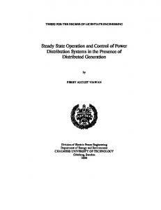
3.3 Data sets (engine manufacturer) The engine manufacturer supplied us with a full set of test data for the specific engine [38]. The test protocol includes the following variables: Engine speed Engine load Fuel flowrate per cylinder/stroke Fuel Injection system parameters In cylinder pressure and temperature Intake and exhaust line temperatures and pressures Air filter operation characteristics Diesel Particulate Filter operation characteristics The set of manufacturer’s operation points was selected to cover the full load curve of the operation map (see Figure 12). 260 2850 2650
240
2450 220 200
2050
180
1850 1650
160
Engine Speed 1450
Engine Torque
Engine Torque [Nm]
Engine Speed [rpm]
2250
140
1250 120
1050
100
850 0
1
2
3
4 5 Operation Points
6
Figure 12 Manufacturer full load operation points for the model calibration
7
8
9
3.4 Data sets (inhouse) A succession of steady state operation points was selected for the in‐house tests, as shown in Figure 13. The set of operation points was selected to cover the full extent of the engine operation map (from low speed – low load to high speed‐ high load), and thus study also engine operation that is not represented in the legislated cycles (e.g. NEDC), which usually focus to the lower left quadrant of speed – load regime. The specific sequence of operation points was programmed in the dyno controller (Test Sequence Editor). The transition time between each two successive points was set to 5 seconds.
21
250 Engine Speed
Engine Torque
2500 200
150 1500 100 1000
Engine Torque [Nm]
Engine Speed [rpm]
2000
50
500
0
0 0
1
2
3
4
5
6
7
8
9
10
11
12
13
14
Operation Points Figure 13 Sequence of operation points selected for the comparison of fuels
15
4 The GT‐SUITE One Dimensional Engine Simulation Software 4.1 Overview GT‐SUITE is a well‐known engine simulation tool used by engine makers and suppliers. It is suitable for analysis of a wide range of issues related to vehicle and engine performance. GT‐SUITE is routinely used by engine and vehicle makers and their suppliers. It is also used for ship and power‐ generation engines, small 2 and 4 stroke engines and racing engines (F1, NASCAR, IRL etc). The GT‐SUITE environment provides a useful set of high‐productivity features for pre and post processing, DOE/optimization, neural networks and control modeling. Its usefulness is further enhanced by integration with STAR‐CD, Fluent, Simulink and MS/EXCEL [13, 39]. The model core is based on one dimensional fluid dynamics approach, representing the flow and the heat transfer in the piping and other flow components of an engine. These components are linked together with connection objects. Within the components the properties must be defined by the user. In addition to the fluid flow and heat transfer capabilities, the computational code contains many other specialized models required for engine system analysis. All aspects of the engine below and more can be modeled. GT‐SUITE features an object‐based code design aiming to provide a powerful model building facility and reduce user effort. Models are built in a graphical user interface, GT‐ISE, Integrated Simulation Environment, common to all applications which simplifies the task of synthesizing object libraries and building, editing, executing and post‐ processing models. GT‐ISE minimizes the amount of input data entry, as only unique geometrical elements must be defined. GT‐SUITE is specifically designed for both steady state and transient simulations. In addition it can be used for analysis of engine/powertrain control. GT‐POWER [39] is available as a standalone tool, or coupled with GT‐DRIVE, GTFUEL and GT‐COOL as the GT‐SUITE/flow product. Figure 14 indicates the distinct components in GT‐SUITE:
22
GT‐SUITE GT‐VTRAIN VALVETRAIN KINEMATICS QUASY‐DYNAMIC ANALYSIS MULTI‐BODY DYNAMICS
GT‐FUEL
GT‐COOL
INJECTION SYSTEMS HYDRAULICS
COOLANT SYSTEM THERMAL MANAGEMENT
GT‐POWER ENGINE PERFOMANCE INTAKE/EXHAUST NOISE 3‐D CFD CONTROL AFTERTREATMENT
GT‐DRIVE DRIVELINE‐VEHICLE DYNAMICS DRIVING CYCLE SIMULATION CONTROL
GT‐CRANK RIGID AND ELASTIC DYNAMIC ANALYSIS OF CRANKSHAFTS Figure 14 GT‐SUITE components [40]
4.2
Software applications
GT‐POWER can be used for a wide range of applications relating to engine design and development. Typical applications are analytically presented in the following list figures: Intake and exhaust manifold design and modifying Intake and exhaust valve profile and timing optimization Intake and exhaust line acoustic analysis Design and optimization engine cooling System Design and optimization engine lubricating System Turbocharger matching, wastegate controller, bypasses (Figure 16) EGR system performance – EGR controller Manifold wall temperatures Combustion analysis (Figure 15, Figure 17) Thermal analysis of cylinder components (Figure 18) Design and optimization of active and passive control systems Intake and exhaust line acoustic analysis Design of resonators and silencers for noise control Transient turbocharger response Aftertreatment systems Three Dimensional Computational Fluid Dynamics studies (Star–CD or FLUENT) (Figure 19) Driveline – vehicle dynamics Crankshaft dynamic analysis Figure 15 and Figure 17 presents the simulation results of a turbulent flame model in Spark Ignition engine and the NOx concentration results of a diesel engine using DI Diesel Jet model respectively. Figure 18 indicates the thermal analysis results of cylinder components. Figure 19 presents the 3‐D discretization tool which allows model building based on imported CAD files.
23
Figure 15 Spark Ignition Turbulent flame model [1]
Figure 16 Compressor Efficiency Map DI Diesel jet model [1]
24
Figure 17 DI Diesel jet model [1]
Figure 18 Temperature distribution in cylinder structure[1]
25
Figure 19 3‐D Discretization Tool allows model building based on imported CAD files [1]
Figure 20 Post Injection – puddling model [1]
4.3 GTSUITE solver GT‐SUITE can be used to predict either steady‐state or transient behavior of engine systems. Results include time dependent quantities are presented below: Engine power, torque and volumetric efficiency Flow rates and flow velocities Temperatures in the engine system Pressures in the engine system Internal Combustion Engines emissions Aftertreatment chemistry Noise analysis The solver calculates the mass and energy flow through the different components and the results of the calculations are shown in a post‐processor, GT‐POST. GT‐POST is a user‐friendly interactive post‐processing tool which can be used to manipulate and view all of the plot data generated by a GT‐SUITE simulation [13]. Engine performance can be studied by analyzing mass, momentum and energy flows between engine components and the heat and work transfers within each component.
26
4.3.1 Computational Fluid Dynamics Governing Equations One Dimensional Flow Simulation model involves the solution of Navier‐Stokes equations, conservation of continuity, momentum and energy equations in the direction of mean flow. The time integration methods include an explicit and an implicit integrator [13]. Taking into account the explicit method, the primary solution variables are mass flow, density and internal energy. On the other hand, using the implicit integrator the primary solution variables are flow, pressure and total enthalpy. Entire system’s control volume is discretized into many subvolumes, where each flow object, such as flowsplit, pipe, is represented by a single volume or divided into one or more smaller volumes. These volumes are connected by boundaries. According to principles of Finite Control Volume method, the scalar variables which are pressure, density, enthalpy, concentration, are considered to remain uniform over each computational volume. The vector variables, mass flux, velocity, mass fraction fluxes etc, are calculated for each boundary. The conservations equations solved by GT‐SUITE are shown below: Mass conservation is defined as the rate of change in mass within a subsystem which is equal to the sum of m dm dm = (4.1) from the system : Continuity: m dt boundaries dt Energy conservation is defined as the rate of change of energy in a subsystem is equal to the sum of the energy transfer of the system: d(me) dV ) hA (T Energy : ) (exp licit solver ) (4.2) p (mH T s fluid wall dt dt boundaries
Enthalpy :
d(HV ) dp ) hA (T V (mH T ) (imp licit solver ) (4.3) s fluid wall dt dt boundaries
Momentum conservation, the net pressure forces and wall shear forces acting on a sub system are equal to the rate of change of momentum in the system: u u dxA 1 ) 4C f dpA (mu C p u u A 2 2 D dm boundaries (4.4) Momentum : dt
where: m m V p
A A s e
H h T
fluid
dx
mass flow rate into volume, m volume mass volume pressure density
Au
cross‐section of flow area heat transfer surface area total internal energy total enthalpy heat transfer coefficient fluid temperature
T wall
wall temperature
Cf
skin friction coefficient
Cp
pressure loss coefficient
D
equivalent diameter length of mass element in the flow direction (discretization length) pressure differential acting across dx
dx dp
27
Flow Solution Methods Explicit method fundamentals In the explicit method, the right hand side of the above equations is calculated using values from the previous time step. This yields the derivative of the primary variable and allows the value at the new time to be calculated by integration of that derivative over the time step. In addition, the explicit solver uses only the values of the subvolume in question and its neighboring subvolumes. Important issue to obtain numerical stability is the time step restriction in order to satisfy the Courant condition. This method requires small time steps which are undesirable for long time simulations. Explicit method will produce more accurate predictions of pressure pulsations that occur in engine air flows, fuel injection systems and prediction of pressure wave dynamics is important. The exception is the simulation of the thermal response of an exhaust system from a cold start without the engine. The calculation procedure of this method is described by the following steps: Continuity and energy equations yield the mass and energy in the volume With the volume and mass known, the density is calculated yielding density and energy The equations of state for each species define density and energy as a function of pressure and temperature. The solver will iterate on pressure and temperature until they satisfy the density and energy already calculated for this time step. It is also possible for species change. The transfer of mass between species is also accounted for during this iteration.
The explicit solver includes a one‐dimensional homogeneous equilibrium cavitation model which includes the effect vapor bubble transport. Generally, any vapor bubbles generated are assumed to be uniform distributed in the subvolume. Implicit method fundamentals The implicit method solves the values of all subvolumes at the new time simultaneously, by solving a system of algebraic equations. This approach requires more time per step, but the stability is much greater and so longer time steps may be taken. Another characteristic of this method is the larger time steps, so computational time added per time step is less than the time saved by taking larger steps., Due to this, the implicit method is used for long duration simulations, such as cooling and exhaust warm‐up simulations. Quasi steady method fundamentals There is another one method, the Quasi steady method. This method assumes that spatial changes are much greater than temporal ones, and therefore the 1D governing equations can be considerably simplified. The Quasi‐ steady solver is an imposed flow model, which results in a computationally efficient solution. The flow rate is imposed, not predicted. In both the explicit and implicit solvers pressure is the 'driving' force behind the solution, and the flow rate is predicted. On the other hand, in the quasi‐steady method mass flow is the 'driving' force, and the pressure is predicted. The solution does not solve full transient terms (full momentum), and as a result becomes extremely numerically efficient. Friction, heat transfer, and wall temperature solver are all solved by the same method as the previous solvers. Time Discretization The flow solution is carried out by integration of the conservation equations in both space and time. As presented above, this integration can be explicit, implicit or quasi steady. The time step calculation varies according to the used solution method. Explicit method In this method the calculation is direct and does not require iteration. In order to obtain numerical stability, the time step must be restricted to satisfy the Courant–Friedrichs–Lewy condition (CFL condition) [41]. The relation between the time step and the discretization length is determined by the Courant number, when the explicit solver is used. The time step is limited by this condition, which restricts the time step to be less than 0.8 of the time required for the pressure and flow to propagate across any discretized volume: t u c 0.8 m (4.5) , x
where t :time step [s], x : minimum discretized element length [m], u : fluid velocity [m/s], c :sound speed [m/s], m : time step multiplier specified by the user in RunSetup.
28
Implicit method In this method, the time steps are typically large enough that the computational time added per time step is less than the time saved by taking larger steps. While it has a significant advantage in terms of speed, the implicit solver should be used only in simulations that attain both of the following criteria: There are minimal wave dynamics in the system, or accurate prediction of wave dynamics is unimportant, AND The maximum Mach number in the system is less than 0.3 The time step used by the implicit method is not determined by GT‐SUITE, as in the explicit method, but imposed by the user. Quasi steady method In this method, the time step is imposed by the user or by the wall temperature calculation interval used by the wall temperature solver. For this method, the flow solution time step is the smallest value of the time step in the flow control and the wall temperature calculation interval in the thermal control setup. Length Discretization As mentioned above, discretization is the splitting of large parts into smaller sections In order to improve simulation’s accuracy. There are two discretization ways [13], the first is to break the system up into several different components such as several pipes and/or flowsplits. The second is by discretizing a ‘Pipe’ part in to multiple sub‐volumes, each performing their own calculations. Important issue is the choice of the appropriate discretization length. The discretization lengths will affect computational time. For both the explicit and implicit solution methods, computational time will be higher for smaller discretization lengths, because there will be more sub‐volumes in the system that require calculation of pressure, temperature, etc. In other words, there are more solution variables. In the explicit solution method, the discretization length also affects the simulation time step. The time step is proportional to the discretization length due to the Courant condition discussed previously. Smaller discretization lengths will require smaller time steps, and thus more computational time. For the implicit solution method, the time step is imposed as a constant value, and therefore simulation time is just a function of the number of subvolumes in the system.
4.3.2 Internal Combustion Engine Simulation Model Technical information need to build an Engine Model A variety of data are necessary to build a multiparametric engine model, since internal combustion engines consist of several components. The following list is indicative of the data that is necessary to compile: Engine characteristics: compression ratio, firing order, cylinder configuration, engine type Cylinder Geometry: bore, stroke, connecting rod length, pin offset, piston TDC clearance height, head bowl geometry, piston area, and head area. Intake and Exhaust System: geometry of all components such as manifolds, runners, ports, Aftertreatment systems, tailpipe, and mufflers. Information includes lengths, internal diameters, volumes, and configurations. Additional data on head loss coefficients and discharge coefficients. Intake and Exhaust valves: valve diameter, lift profile, discharge coefficient in both directions, swirl coefficient, tumble coefficient, valve lash Combustion analysis and heat transfer: Wiebe and Woschni model respectively Throttles: throttle location and discharge coefficients versus throttle angle in both flow directions. Fuel Injection system: location and number of injectors, number of nozzle holes and nozzle diameter, air to fuel ratio (A/F ratio), fuel type (gasoline, diesel, biodiesel) and fuel properties (viscosity, density, Lower Heating Value) and injection characteristics, such as number of pulses injection rate, injection timing, injection pressure, and injection duration. Turbocharger component: turbine and compressor maps, turbocharger inertia, performance characteristics at several engine operating conditions (Pressure Ratio, turbine and compressor speed, compressor inlet pressure and temperature) EGR Valve: EGR valve diameter, EGR angle and EGR fraction Wastegate Controller: Wastegate diameter, target boost pressure. Ambient State: Ambient operating conditions such as temperature, pressure and humidity.
29
4.3.2.1 Engine layout A typical engine is modeled using 'EngCylinder' and 'EngineCrankTrain' component objects and 'ValveConn' and 'EngCylConn' connection objects. The most common objects, 'EngCylinder' and 'EngineCrankTrain', are used to define the basic engine geometry and characteristics. Both objects refer to several reference objects for more detailed modeling information on aspects such as combustion and heat transfer. Cylinders must be connected to the engine with 'EngCylConn' parts. Cylinders are connected to intake and exhaust ports with 'ValveConn' connections. Many 'ValveConn' connection templates are available to define different types of valves and their characteristics. Four‐Stroke engines are the most common in the automotive industry but in some applications are used two‐ stroke engines. This engine type can be also modeled via GT‐SUITE software package. Two stroke engines have some unique engine components in addition to those of four‐stroke engines (e.g. while two stroke engines may use cam‐ driven valves, they typically have ported valves connected to the crankcase). A crankcase is defined using an 'EngCrankcase' object. Crankcases are attached to the engine with an 'EngCrkConn' connection to calculate engine flow and scavenging. This connection connects the crankcase to the cylinder. Additionally, the inlet to the crankcase often has a reed valve that is used to check the airflow. This valve is modeled by a 'ValveCheckConn' object. The instantaneous position of the reed valve is calculated from the pressure differential across the valve [42].
4.3.2.2 Intake and exhaust camshafts Intake and exhaust camshafts can be modeled by a lot of 'Valve*Conn' templates. There are different templates available, related to the cylinder valve types (cam driven, solenoid valves): 'ValveCamConn', 'ValveCamDesginConn', 'ValveCamDynConn', 'ValveCamPRConn' and 'ValveCamUserConn''. In our model, we used the most common template, 'ValveCamConn' [42]. Its characteristics will be presented in the following chapter. Most of the available templates use a discharge coefficient to describe the valve flow area. Important parameter for the calculation of discharge coefficients is the reference valve diameter. The valve cam part is the part that represents the intake and exhaust valves in the GT‐Suite model. The valve cam part is connected to the cylinder part. This object defines the characteristics of a cam‐driven valve including its geometry, lift profile and flow characteristics. The valve angle and lift array data should be consistent with the angle and lift attributes so that valve position, φ, is specified relative to TDC firing as in the following equations: standard: φTDCF =φarray *AngleMultiplier+CamTimingAngle (4.6)
opening:φTDCF =(φarray ‐φfdp )*AngleMultiplier+CamTimingAngle+φfdp (4.7) closing:φTDCF =(φarray ‐φldp )*AngleMultiplier+CamTimingAngle+φldp (4.8) opening:φTDCF =(φarray ‐φml )*AngleMultiplier+CamTimingAngle+φml (4.9)
Where φarray represents the array of angles where the valve is open, φ fdp is the first data point, φldp the last point
and φml is the maximum lift. The main settings are: Valve Reference Diameter Valve Lash Cam Timing Angle The valve reference diameter is used to calculate the effective flow area from the discharge coefficient arrays. This diameter does not need to specifically correspond to one geometric characteristic of the valve (for example valve face, valve seat) but has to exactly correspond with the reference diameter used to calculate the discharge coefficients. The valve lash is the mechanical clearance between the cam lobe and valve stem. There are also some optional settings for the valves. There is a cam driver that can give a phasing angle to the valve event relative to global crank angle. This attribute enables each valve to be phased according to firing order and interval without having to reassign a different cam timing angle. In our case the valves are directly connected to the engine cylinders and therefore automatically be set to the firing order [42]. Then a series of multipliers can be used: Flow Area, Angle, Lift, Swirl, and Tumble.
30
4.3.2.3 Intake and exhaust cylinder ports The intake and exhaust cylinder ports can be modeled geometrically with pipes. There are some considerations for wall temperature, heat transfer multiplier and friction multiplier. Especially for the exhaust valve ports, successful modeling is very important since wall temperatures change substantially between full and idle conditions, thus influencing the turbine inlet temperature and power and compressor’s reaction.
4.3.2.4 Fuel injection system Fuel injection is modeled by means of various templates depending on the engine type and the injector location: 'InjAFSeqConn': Typically, this injector connection is used to model sequential fuel injection in SI gasoline engines. This injector would be used when one knows the injector delivery rate and the desired fuel ratio. An important output of this injector is the calculated pulse width. This injector is ideal for developing baseline fuel maps. The user imposes injector known properties and the desired fuel ratio at each map operating condition. When the delivery rate of the injector is not known, it can be estimated using the following equation: 6 delivery nv ref VD (F / A) (4.10) m Nc ti where: delivery m injector delivery rate [g/s] nv
ref VD
F/A Nc ti
volumetric efficiency [fractional] reference density for volumetric efficiency [kg/m3]
engine displacement [liter] fuel to air ratio number of cylinders injection duration [CA]
'InjProfileConn': This template is the most commonly used to inject fuel directly into the cylinders of diesel or GDI (gasoline direct injection) engine models. This injector should always be used for direct‐injection diesel engines. Pilot injection can be also modeled using this injector. 'InjAF‐RatioConn': This injector connection is used typically to model carburetors in SI gasoline engines. It injects fuel at a constant fuel‐to‐air ratio. It gives options to sense the airflow rate "locally" at the site of the injector For local fuel injection, the injection is idealized so that the imposed F/A ratio is always realized, even if the velocity at the point of injection reverses. 'InjPulseConn': This connection is commonly used for SI gasoline engines to model sequential fuel injection. This injector would be used if one knows the injector delivery rate and the injection pulse width.
There are also other injection templates such as, 'InjRateConn', 'InjMeanValueConn', 'InjNozzConn'(prediction of cavitation losses in injectors), 'InjNozzleUserConn'(predictive injection model implemented by user) [42].
4.3.2.5 Throttle and EGR valve This template describes a throttle placed between two flow components. The user imposes the throttle angle, according to which the effective area of the throttle. This object is typically only used when measured discharge coefficient data is available from a flow bench test. Unfortunately, like our simulation, discharge coefficient data is not available. Therefore, one must consider alternative ways to model the throttle. Taking into account [43] there are two main approaches that are used to account for the throttle: Approach 1: If the simulation work will be done for wide‐open throttle only, then an 'OrificeConn' can be used to obtain the desirable pin size. It should be mentioned that this throttle pin at wide‐open throttle typically occupies about 15% or more of the throttle body area. Next step is the setting of the orifice diameter so that its area equals the area of the wide‐open throttle and the discharge coefficients to 1.0. The equivalent orifice diameter can be found by the following equation:
31
4 Dthrottle 2 TDthrottle (4.11) , where: Deq is the equivalent diameter of the wide open throttle, Dthrottle is 4 the throttle body diameter and T is thickness of the wide‐open throttle valve and pin. Approach 2: If the simulation work includes part load, implement an 'OrificeConn' or 'ThrottleConn' component at the location of the throttle and use a 'PIDController' – 'Throttle Controller' component to impose the desired part‐ load quantity such as BMEP, brake torque, or intake manifold pressure. Deq
4.3.2.6 Combustion and emissions GT‐Suite provides many different combustion model alternatives. For a given engine type there are multiple available models and the user may select the most appropriate for his specific application. The primary decision is whether the model will be non‐predictive, semi‐predictive or predictive. There are significant differences between the combustion models which are presented in the following table: Table 3 Computed combustion models [42] Non ‐ Predictive model Semi – Predictive model Predictive model Imposed burn rate as a function of Good substitute for a predictive Theoretically, the most appropriate crank angle model. model. Substantially slower: complexity of Sensitive to the variables that the calculations leads to higher Appropriate for no prediction of influence combustion rate. Utilize computational time. burn rate modeling. Applications a non‐predictive methodology Higher model implementation where the investigated variables where burn rate is imposed but effort: require more data which have minimal effect on the burn employ methods to calculate the should be calibrated to measured rate. proper Wiebe parameters. data and implemented in the model. Non appropriate for predicted burn Implement predictive models only Much less CPU intensive and rate modeling, where the variables when required. Otherwise, sometimes more accurate than have significant effect on the burn implement non‐predictive model predictive rate. whenever appropriate. As mentioned above, there are a lot of combustion models which simulated by an appropriate template. The following templates are available for non‐predictive models: 'EngCylCombProfile': Imposed combustion profile 'EngCylCombSIWiebe': Spark ingintion Wiebe model 'EnCylCombWiebe': Direct injection diesel Wiebe model 'EngCylCombMultiWiebe': Multiwiebe model There are also available templates for predictive and semi – predictive models: Predictive models 'EngCylCombSITurb': Spark ignition turbulent flame model 'EngCylCombDIJet': Direct injection diesel jet model 'EngCylCombHCCI': Homogeneous Charge Compression Ignition model 'UserModel': User combustion model 'EngCylKIVA': KIVA external cylinder model Semi‐predictive models Semi‐predictive SI combustion Semi‐predictive diesel combustion The last semi‐predictive model is presented below:
32
'EngCylCombDIWiebe', normally non‐predictive model, imposes the burn rate for direct‐injection, compression‐ ignition engines using a three‐term Wiebe function, the superposition of three normal Wiebe curves. These Wiebe curves approximate the "typical" shape of a DI compression ignition burn rate. The purpose of using three functions is to make it possible to model pre‐ignition and larger tail. This model should be used only [42] when the fuel is injected directly into the cylinder with an 'InjProfileConn' connection. When the Wiebe functions are imposed, the injection profile will not influence the burn rate except if, at any instant, the specified cumulative combustion exceeds the specified injected fuel fraction. This model provides a convenient means of implementing a reasonable burn rate if measured cylinder pressure is not available. If cylinder pressure has been measured, 'EngCylCombProfile' will typically provide a more accurate burn rate. The Wiebe equations are given below: Inputs: SOI = Start of Injection, ID = Ignition Delay, DP = Premix Duration, DM= Main Duration DT = Tail Duration, FP =Premix Fraction, FT = Tail Fraction, E P = Premix Exponent, EM =Main Exponent ET =Tail Exponent, CE =Combustion Efficiency Calculated constants: FM =Main Fraction, WCP =Wiebe Premix Constant, WC M = Wiebe Main Constant, WCT =Wiebe Tail Constant The relation between the fractions is given below: FM (1 Fp FT ) (4.12) The calculated constants are presented in the following equations:
DP WCP 1/(EP 1) 1/(EP 1) 0.105 2.302
(EP 1)
DM (4.13) , WCM 1/(EM 1) 1/(EM 1) 0.105 2.302
(EM 1)
(4.14)
(E 1)
T DT WCT (4.15) 1/(E 1) 1/(E 1) 2.302 T 0.105 T The 'EngCylCombDIWiebe' template becomes semi‐predictive if the user specifies "def" for the ignition delay or Wiebe attributes. Attributes set to "def" will be calculated from the injection profile, air‐to‐fuel ratio, pressure, and temperature [42]. In order to obtain meaningful results when "def" has been entered, the injector geometry and injection pressure profile must be precisely specified because they will affect the burn rate. According to [42], this model is not valid for simulations at idle, with fuels other than diesel and EGR higher than 15%. GT‐Suite offers to the user the capability to model exhaust emissions like, N2, O2, CO2, CO, H2O, H, O, OH, NO, N.
4.3.2.7 Air boxes and Air filters Internal combustion engines is equipped with an air box / filter assembly in the intake system. The air box has a cross section that is significantly larger than the inlet and outlet pipes and contains an air filter. Air box has an important effect on intake pressure drop and acoustic behavior, and is therefore an important part of the engine model. For simple geometry, single chambers, air box can be modeled with a simple 'Pipe' or 'FlowSplit' object. On the other hand, for more complex and realistic geometry, the air box volume can be modeled by two or more connected flowsplits. Even with the simple representation, the most significant pressure drop occurs at the expansion into the chamber and contraction at the chamber outlet and the pressure drops are captured [42]. It should be mentioned that, the pressure drop across the filter is usually small relative to the expansion/contraction pressure losses and for that reason the filter is generally ignored. Generally, the filter is folded in order to increase the effect flow area through the filter minimizing, if not eliminating the influence it has on the pressure loss in the air box.
4.3.2.8 Mufflers and silencers Typical exhaust muffler has a large cross section making in order to allow pressure waves to travel in more than one dimension. Typically, mufflers and silencers involve large volumes that contain internal pipes and other elements to reduce exhaust noise and several sound frequencies. At this engine part one dimension Navier‐Stokes equations is also solved [42].
33
4.3.2.9 Intercoolers and EGR Cooler GT‐SUITE offers various ways to model an intercooler or EGR cooler depending on the application. There are 3 main categories of models: non‐predictive, semi‐predictive and predictive [42]. In non‐predictive model the outlet temperature of the intercooler may be imposed by modeling the intercooler as an infinite sink of heat, using a multiple pipe object that is created from the 'Pipe' template. The wall temperature and the friction and heat transfer multipliers of the pipe object can be imposed by the user on order to obtain the desired outlet temperature and pressure drop. On the other hand, many intercooler suppliers rate the performance of their heat exchangers using "effectiveness", which is the ratio of the actual temperature reduction through the intercooler to the maximum possible reduction in temperature. Many turbocharger matching techniques predict outlet temperature using this effectiveness. It is possible to use controls to calculate the outlet temperature of the intercooler and impose this value in a non‐predictive intercooler model. This technique is considered "semi‐predictive" because it will not take into account differences in fluid density in operation compared to the fluid density during the measurement of effectiveness. In conclusion, the heat exchanger performance, including the fluid conditions on the coolant side, may also be predicted using measured heat transfer data. In this model, 'HxMaster' template models the internal side of the intercooler. Moreover, the conditions on the external side of the intercooler can be imposed either in the 'HxMaster' template itself or from an 'HxSlave' template in the coolant flow circuit that is connected to 'HxMaster'.
4.3.2.10
Controllers
The most common controller is PID controller. There is ' PIDController' template which contains a continuous proportional‐integral‐derivative (PID) controller. Its purpose is to achieve and maintain a target value of some sensible quantity from the system (also known as the "plant") by controlling some input to the plant. The sensed value from the plant is the input signal to the controller, and the output signal controller from the 'PIDController' is used to "control" some actuatable device on the plant. This type of control configuration is known as "closed‐loop control" because the signals make a loop between the plant and the controller. There are many applications for a PID controller and the most [43] common engine‐related are presented below: Target engine torque by controlling throttle angle for SI engines. Target engine torque by controlling injection rate for DI engines. Target boost pressure by controlling turbine wastegate diameter or turbine rack position. Target EGR fraction by controlling the EGR valve. Target coolant temperature by controlling a radiator‐bypass valve. Target air‐to‐fuel ratio by controlling pulse width and/or solenoid duration. Target vehicle speed by controlling the actuator pedal position.
4.3.2.11
Aftertreatment Exhaust Systems
Modeling of exhaust aftertreatment systems can be a challenge taking into account the complex nature of chemical reactions and the sensitivity of a system to the exhaust gas composition, pressure and temperature. The investigation can be break up into the following parts: back pressure, acoustics, gas temperatures and chemical reactions. GT‐POWER includes the capability to model numerous exhaust aftertreatment components and complete aftertreatment systems. The methodology is highly flexible and gives the user complete control over the reaction kinetics that is to be used. The kinetics is not hard‐wired, nor do they require the user to modify user subroutines. The kinetics is user‐defined via an intuitive Graphical User Interface The modeling possibilities include: Single stand alone exhaust aftertreatment component. Multiple exhaust aftertreatment components in series or parallel Integration of controls with exhaust aftertreatment Full model integration of engine model + exhaust aftertreatment model + driveline model + more 3‐way catalyst model and an oxidation catalyst model Internal kinetic mechanisms assembler and stiff kinetics solver Linkage to external kinetics codes, e.g. CHEMKIN Properties of standard GT‐POWER species have been designed to be compatible with CHEMKIN Users can add new species from CHEMKIN‐format data files
34
The basic structure of the Aftertreatment (Catalyst) Modeling methodology is presented in Figure 21:
EXTERNAL CHEMISTRY MODEL
USER MODEL
From Engine Pollutant Source
Chemical Kinetics Tool Box
GT‐POWER CATALYST BRICK
Built‐in ODE Solver
Figure 21 Aftertreatment: Catalyst Modeling in GT‐SUITE [1]
4.3.2.12
To Tailpipe
Speed specification versus load specification
The performance of an engine can be determined by either resolving engine brake torque for an imposed engine speed or by solving both the engine speed and engine brake torque for an imposed load torque. The user chooses the simulation specification. This mode is imposed via 'EngineCrankTrain' object. Information for each simulation mode is presented below: Speed mode is the most commonly used mode of engine simulation, especially for steady state cases. Taking into account [42], this method provides very quickly results because the engine speed is imposed from the start of the simulation. Load mode allows the user to impose a load on the engine or to couple the engine to a vehicle model so that the speed of the engine will be calculated.
4.4 Turbochargers Various types of exhaust‐driven turbocharger have been designed for supercharging reciprocating internal combustion engines. A turbocharger consists basically of a compressor and a turbine coupled on a common shaft. The exhaust gases from the engine directed by the turbine inlet casing on the blades of the turbine and subsequently discharged to atmosphere through a turbine outlet casing [44]. The exhaust gases are utilized in the turbine to drive the compressor, which compresses the air and directs it to the engine induction manifold, to supply the engine cylinders with air of higher density than is available to a naturally aspirated engine. The combination of a single‐stage centrifugal compressor and a single‐stage axial flow or radial flow turbine is almost universally used in turbochargers [44]. The former type with the axial flow turbine is used for most of the medium and large size engines suitable for rail, industrial and marine purposes and the latter type with the radial flow turbine foe small engines of the automotive type. This type of turbocharger is presented in Figure 23. The turbocharger's basic functions have not fundamentally changed since the times of Alfred Büchi. It must be mentioned that the first exhaust‐driven supercharger [45], which is shown in Figure 22 was developed by Dr. Alfred J. Büchi of Switzerland between 1909 and 1912. On 16 November 1905 Dr. Alfred Büchi received patent No. 204630 from the Imperial Patent Office of the German Reich for a "combustion machine consisting of a compressor (turbine compressor), a piston engine, and a turbine in sequential arrangement”.
35
Figure 22 Cutaway of first exhaust‐driveen superchargger pressor and a turbine conn nected by a co ommon shaftt. The exhaustt‐gas‐driven A turboccharger consissts of a comp turbine supp plies the drive energy for th he compressorr. Compressor Turbine Control system Bearing ssystem
Figure 23 Cutaway of com mmon turbocharger [46]
4.4.1 Co ompresso or stall A compre essor stall is aa situation of aabnormal airfflow resulting from a stall o of the aerofoills within the ccompressor. Stall is found d in dynamic compressors,, particularly axial compresssors, as used d in jet enginees and turbocchargers for reciprocatingg engines Compressor stalls resu ult in a loss of o compresso or performancce, which can n vary in seveerity from a momentary urring so quiickly it is barrely registere ed on engine instruments) to a complete loss of engine poweer drop (occu compression n (compressorr surge) necessitating a redu uction in the ffuel flow to th he engine. Modern compressors are carefully designed and d controlled to t avoid or lim mit stall with hin an engine''s operating was a commo on problem on n early jet engines with sim mple aerodyn namics and manual or mecchanical fuel range. Stall w control unitss, but has been virtually eliminated e byy better desiggn and the usse of hydromechanical and d electronic control systeems such as Fu ull Authority D Digital Engine Controls. There aree two types off compressor stall [46]:
3 36
Rotational stall is a local disruption of airflow within the compressor which continues to provide compressed air but with reduced effectiveness. Rotational stall arises when a small proportion of aerofoils experience aerofoil stall disrupting the local airflow without destabilising the compressor. The stalled aerofoils create pockets of relatively stagnant air (referred to as stall cells) which, rather than moving in the flow direction, rotate around the circumference of the compressor. The stall cells rotate with the rotor blades but at 50%‐70% of their speed, affecting subsequent aerofoils around the rotor as each encounters the stall cell. Stable local stalls can also occur which are axi‐symmetric, covering the complete circumference of the compressor disc but only a portion of its radius, with the remainder of the face of the compressor continuing to pass normal flow. A rotational stall may be momentary, resulting from an external disturbance, or may be steady as the compressor finds a working equilibrium between stalled and unstalled areas. Local stalls substantially reduce the efficiency of the compressor and increase the structural loads on the aerofoils encountering stall cells in the region affected. In many cases however, the compressor aerofoils are critically loaded without capacity to absorb the disturbance to normal airflow such that the original stall cells affect neighboring regions and the stalled region rapidly grows to become a complete compressor stall. Axi‐symmetric stall, more commonly known as compressor surge; or pressure surge, is a complete breakdown in compression resulting in a reversal of flow and the violent expulsion of previously compressed air out through the engine intake, due to the compressor's inability to continue working against the already‐compressed air behind it. The compressor either experiences conditions which exceed the limit of its pressure rise capabilities or is highly loaded such that it does not have the capacity to absorb a momentary disturbance, creating a rotational stall which can propagate in less than a second to include the entire compressor. The compressor will recover to normal flow once the engine pressure ratio reduces to a level at which the compressor is capable of sustaining stable airflow. If, however, the conditions that induced the stall remain, the return of stable airflow will reproduce the conditions at the time of surge and the process will repeat.[1] Such a "locked‐in" or self‐reproducing stall is particularly dangerous, with very high levels of vibration causing accelerated engine wear and possible damage, even the total destruction of the engine. Causes Compressor stalls are aerodynamic stalls [44] in which the aerofoils in the compressor are loaded above their lifting capability. This can arise for a number of reasons which result in either a drop in the expected compressor performance or the compressor is loaded in conditions beyond its design. Factors affecting compressor performance
Damaged compressor components caused by ingestion of foreign objects. One of the most common causes of compressor stalls in commercial aviation aircraft is a bird strike. On take‐off, while maneuvering on the ground or while on approach to landing, planes operate in proximity to birds. It is not uncommon for birds to be sucked into the intake of the engine and the disruption to the airflow and damage to the blades often causes compressor stall. Worn or contaminated compressor components such as eroded rotor blades, seals or bleed valves. Even dust and dirt in the compressor can reduce its efficiency and lead to a stall if the contamination is severe enough. Factors increasing compressor loads
Aircraft operation outside of design envelope. E.g., extreme flight man oeuvre resulting in airflow separations within the engine intake. Flight within icing conditions where ice can build up within the intake or compressor. Engine thrust requirements too high for the operating altitude. (limited with modern fly‐by‐wire controls) Engine operation outside specified design parameters. E.g., abrupt increases in engine thrust (slam acceleration) causing a mismatch between engine components. (Occurrence reduced through the use of modern electronic control units.) Turbulent or hot airflow to the engine intake. E.g., use of reverse thrust at low forward speed, resulting in re‐ingestion of hot turbulent air, or for military aircraft, ingestion of hot exhaust gases from fired missile. Worn or contaminated engine components. E.g., poorly performing control unit or turbine within an engine may result in a mismatch increasing the likelihood of stall.
37
Effects Compressor axially‐symmetric stalls, or compressor surges, are immediately identifiable because they produce one or more extremely loud bangs from the engine. Reports jets of flame emanating from of the engine are common during this type of compressor stall. These stalls may be accompanied by an increased exhaust gas temperature, an increase in rotor speed due to the large reduction in work done by the stalled compressor and yawing of the aircraft in the direction of the affected engine due to the loss of thrust. Severe stresses occur within the engine and aircraft particularly from the intense aerodynamic buffeting within the compressor. Response and recovery The appropriate response to compressor stalls varies according the engine type and situation, but usually consists of immediately and steadily decreasing thrust on the affected engine. While modern engines with advanced control units can avoid many causes of stall, jet aircraft pilots must continue to take this into account when dropping airspeed or increasing throttle.
4.4.2 Design and function of compressor The radial flow (centrifugal) compressor is made up from four basic components [44]: a stationary inlet casing which in some applications provided with an air filter and noise reducing baffles a rotating impeller a stationary diffuser of the vaneless or vaned the collector or volute
Figure 24 Diagrammatic sketch of radial compressor [47] Guide vanes have been fitted in the inlet casing of some compressors, principally to enable some control to be exercised over the flow characteristics, for example, lowering of the entry Mach number at the impeller eye or shift of the surge line by varying the vane angle. Design and function Turbocharger compressors are generally centrifugal compressors consisting of three essential components: compressor wheel, diffuser, and housing. With the rotational speed of the wheel, air is drawn in axially, accelerated to high velocity and then expelled in a radial direction. The diffuser slows down the high‐velocity air, largely without losses, so that both pressure and temperature rise. The diffuser is formed by the compressor back plate and a part of the volute housing, which in its turn collects the air and slows it down further before it reaches the compressor exit.
38
Operating characteristics The compressor operating behavior is generally defined by maps showing the relationship between pressure ratio and volume or mass flow rate. The useable section of the map relating to centrifugal compressors is limited by the surge and chokes lines and the maximum permissible compressor speed. Surge line The map width is limited on the left by the surge line. This is basically "stalling" of the air flow at the compressor inlet. With too small a volume flow and too high a pressure ratio, the flow can no longer adhere to the suction side of the blades, with the result that the discharge process is interrupted. The air flow through the compressor is reversed until a stable pressure ratio with positive volume flow rate is reached, the pressure builds up again and the cycle repeats. This flow instability continues at a fixed frequency and the resultant noise is known as "surging".
Efficiency islands Surge line
Turbocharger speed lines
Pressure ratio axis
Mass flow axis Choke line
Figure 25 Compressor map of a turbocharger for passenger car application [48] Choke line The maximum centrifugal compressor volume flow rate is normally limited by the cross‐section at the compressor inlet. When the flow at the wheel inlet reaches sonic velocity, no further flow rate increase is possible. The choke line can be recognized by the steeply descending speed lines at the right on the compressor map.
4.4.3 Design and function of a turbine The radial flow turbine consist of a scroll or inlet casing, a set of inlet nozzles followed by a short vaneless gap and the turbine wheel itself. Most small turbocharger turbines use a nozzles casing to improve flow range at some penalty in peak efficiency, but also reducing cost. The nozzles accelerate the flow, reducing pressure and increasing kinetic energy. A short vaneless space prevents the rotor and blades from touching and allows wakes coming off the trailing edge of the nozzle blades to mix out. Energy transfer occurs solely in the impeller, which should be designed for minimum kinetic energy at the exit.
39
Inlet casing
Nozzles
Vaneless space
Rotor Figure 26 Diagrammatic sketch of radial turbine [47] Design and function The turbocharger turbine, which consists of the turbine wheel and turbine housing, converts the engine exhaust gas into mechanical energy to drive the compressor. The gas, which is restricted by the turbine's flow cross‐sectional area, results in a pressure and temperature drop between the inlet and outlet. This pressure drop is converted by the turbine into kinetic energy to drive the turbine wheel. There are two main turbine types: axial and radial flow. In the axial‐flow type, flow through the wheel is only in the axial direction. In radial‐flow turbines, gas inflow is centripetal, i.e. in a radial direction from the outside in, and gas outflow in an axial direction. Up to a wheel diameter of about 160 mm, only radial‐flow turbines are used. This corresponds to an engine power of approximately 1000 kW per turbocharger. From 300 mm onwards, only axial‐flow turbines are used. Between these two values, both variants are possible [46]. As the radial‐flow turbine is the most popular type for automotive applications, the following description is limited to the design and function of this turbine type. In the volume of such radial or centripetal turbines, exhaust gas pressure is converted into kinetic energy and the exhaust gas at the wheel circumference is directed at constant velocity to the turbine wheel. Energy transfer from kinetic energy into shaft power takes place in the turbine wheel, which is designed so that nearly all the kinetic energy is converted by the time the gas reaches the wheel outlet. Operating characteristics The turbine performance increases as the pressure drop between the inlet and outlet increases, i.e. when more exhaust gas is dammed upstream of the turbine as a result of a higher engine speed, or in the case of an exhaust gas temperature rise due to higher exhaust gas energy.
Figure 27 Turbocharger turbine map [46]
40
The turbine's characteristic behavior is determined by the specific flow cross‐section, the throat cross‐section, in the transition area of the inlet channel to the volute. By reducing this throat cross‐section, more exhaust gas is dammed upstream of the turbine and the turbine performance increases as a result of the higher pressure ratio. A smaller flow cross‐section therefore results in higher boost pressures. The turbine's flow cross‐sectional area can be easily varied by changing the turbine housing. Besides the turbine housing flow cross‐sectional area, the exit area at the wheel inlet also influences the turbine's mass flow capacity. The machining of a turbine wheel cast contour allows the cross‐sectional area and, therefore, the boost pressure, to be adjusted. A contour enlargement results in a larger flow cross‐sectional area of the turbine. Turbines with variable turbine geometry change the flow cross‐section between volute channel and wheel inlet. The exit area to the turbine wheel is changed by variable guide vanes or a variable sliding ring covering a part of the cross‐section. In practice, the operating characteristics of exhaust gas turbocharger turbines are described by maps showing the flow parameters plotted against the turbine pressure ratio. The turbine map shows the mass flow curves and the turbine efficiency for various speeds. To simplify the map, the mass flow curves, as well as the efficiency, can be shown by a mean curve For high overall turbocharger efficiency, the co‐ordination of compressor and turbine wheel diameters is of vital importance. The position of the operating point on the compressor map determines the turbocharger speed. The turbine wheel diameter has to be such that the turbine efficiency is maximized in this operating range. Twin‐entry turbines It was the development of the pulse turbocharging in the early ‘30s, patented by its inventor Alfred Büchi in 1925 that was the major breakthrough in the history of turbocharging. Although the constant pressure system is widely used in certain types of engines. The objective is to make the maximum use of the high pressure and temperature which exist in the cylinder at the moment of exhaust valve or port opening, even at the expense of creating highly unsteady flow through the turbine. In most cases the benefit from increasing the available energy will be more than offset the loss in turbine efficiency due to unsteady flow [44]. The turbine is rarely subjected to constant exhaust pressure. In pulse turbocharged commercial diesel engines, twin‐entry turbines allow exhaust gas pulsations to be optimized, because a higher turbine pressure ratio is reached in a shorter time. Thus, through the increasing pressure ratio, the efficiency rises, improving the all‐important time interval when a high, more efficient mass flow is passing through the turbine. As a result of this improved exhaust gas energy utilization, the engine's boost pressure characteristics and, hence, torque behavior is improved, particularly at low engine speeds [46]. To prevent the various cylinders from interfering with each other during the charge exchange cycles, three cylinders are connected into one exhaust gas manifold. Twin‐entry turbines then allow the exhaust gas flow to be fed separately through the turbine.
Figure 28 Turbocharger with twin‐entry turbine [48]
41
The turbine is rarely subjected to constant exhaust pressure. In pulse turbocharged commercial diesel engines, twin‐entry turbines allow exhaust gas pulsations to be optimized, because a higher turbine pressure ratio is reached in a shorter time. Thus, through the increasing pressure ratio, the efficiency rises, improving the all‐important time interval when a high, more efficient mass flow is passing through the turbine. As a result of this improved exhaust gas energy utilization, the engine's boost pressure characteristics and, hence, torque behavior is improved, particularly at low engine speeds. To prevent the various cylinders from interfering with each other during the charge exchange cycles, three cylinders are connected into one exhaust gas manifold. Twin‐entry turbines then allow the exhaust gas flow to be fed separately through the turbine. Water‐cooled turbine housings Turbine housings can be supplied either water cooled or air cooled. The water cooled versions are available for applications where the turbine casing must be kept cool for safety reasons, or whether thermal radiation in a confined space causes problems, for example, locomotive or marine application [44]. In ship engine rooms, for instance, hot surfaces have to be avoided because of fire risks. Therefore, water‐cooled turbocharger turbine housings or housings coated with insulating material are used for marine applications. Commercial turbochargers with water‐cooled turbine housing are presented in Figure 29 .
Figure 29 Turbocharger with water‐cooled turbine housing – Garrett GT 49 (left) and Garrett GT52 (right) [48]
4.4.4 Control system Target and function The drive ability of passenger car turbo engines must meet the same high requirements as naturally aspirated engines of the same power output. That means, full boost pressure must be available at low engine speeds. This can only be achieved with a boost pressure control system on the turbine side. Control by turbine‐side bypass The turbine‐side bypass is the simplest form of boost pressure control. The turbine size is chosen such that torque characteristic requirements at low engine speeds can be met and good vehicle driveability achieved. With this design, more exhaust gas than required to produce the necessary boost pressure is supplied to the turbine shortly before the maximum torque is reached. Therefore, once a specific boost pressure is achieved, part of the exhaust gas flow is fed around the turbine via a bypass. The wastegate which opens or closes the bypass is usually operated by a spring‐loaded diaphragm in response to the boost pressure. Today, electronic boost pressure control systems are increasingly used in modern passenger car diesel and petrol engines. When compared with purely pneumatic control, which can only function as a full‐load pressure limiter, a flexible boost pressure control allows an optimal part‐load boost pressure setting. This operates in accordance with various parameters such as charge air temperature, degree of timing advance and fuel quality. The operation of the flap corresponds to that of the previously described actuator. The actuator diaphragm is subjected to a modulated control pressure instead of full boost pressure. This control pressure is lower than the boost pressure and generated by a proportional valve. This ensures that the diaphragm is subjected to the boost pressure and the pressure at the compressor inlet in varying proportions. The proportional valve is controlled by the engine electronics. For diesel engines, a vacuum‐regulated actuator is used for electronic boost pressure control [44].
42
Figure 30 Boost pressure control of a turbocharged petrol engine by proportional control pressure [46]
4.4.5 Variable turbine geometry The variable turbine geometry allows the turbine flow cross‐section to be varied in accordance with the engine operating point. This allows the entire exhaust gas energy to be utilised and the turbine flow cross‐section to be set optimally for each operating point. As a result, the efficiency of the turbocharger and hence that of the engine is higher than that achieved with the bypass control.
Figure 31 Turbocharger with variable turbine geometry (VTG) [46]
4.4.6 Flow cross-section control through variable guide vanes: VTG Variable guide vanes between the volute housing and the turbine wheel have an effect on the pressure build‐up behavior and, therefore, on the turbine power output. At low engine speeds, the flow cross‐section is reduced by closing the guide vanes. The boost pressure and hence the engine torque rise as a result of the higher pressure drop between turbine inlet and outlet. At high engine speeds, the guide vanes gradually open. The required boost pressure is achieved at a low turbine pressure ratio and the engine's fuel consumption reduced. During vehicle acceleration from low speeds the guide vanes close to gain maximum energy of the exhaust gas. With increasing speed, the vanes open and adapt to the corresponding operating point [44]. Today, the exhaust gas temperature of modern high‐output diesel engines may reach 830 °C. The precise and reliable guide vane movement in the hot exhaust gas flow puts high demands on materials and requires tolerances within the turbine to be exactly defined. Irrespective of the turbocharger frame size, the guide vanes need a minimum clearance to ensure reliable operation over the whole vehicle lifetime.
43
4.4.7 Bearing system The turbocharger shaft and turbine wheel assembly rotates at speeds up to 300,000 rpm. Turbocharger life should correspond to that of the engine, which could be 1,000,000 km for a commercial vehicle. Only sleeve bearings specially designed for turbochargers can meet these high requirements at a reasonable cost.
Figure 32 Turbocharger bearing system (cut‐away model) [46] Radial bearing system With a sleeve bearing, the shaft turns without friction on an oil film in the sleeve bearing bushing. For the turbocharger, the oil supply comes from the engine oil circuit. The bearing system is designed such that brass floating bushings, rotating at about half shaft speed, are situated between the stationary centre housing and the rotating shaft. This allows these high speed bearings to be adapted such that there is no metal contact between shaft and bearings at any of the operating points. Besides the lubricating function, the oil film in the bearing clearances also has a damping function, which contributes to the stability of the shaft and turbine wheel assembly. The hydrodynamic load‐carrying capacity and the bearing damping characteristics are optimized by the clearances. The lubricating oil thickness for the inner clearances is therefore selected with respect to the bearing strength, whereas the outer clearances are designed with regard to the bearing damping. The bearing clearances are only a few hundredths of a millimeter [44, 46]. The one‐piece bearing system is a special form of a sleeve bearing system. The shaft turns within a stationary bushing, which is oil scavenged from the outside. The outer bearing clearance can be designed specifically for the bearing damping, as no rotation takes place. Axial‐thrust bearing system Neither the fully floating bushing bearings nor the single‐piece fixed floating bushing bearing system support forces in axial direction. As the gas forces acting on the compressor and turbine wheels in axial direction are of differing strengths, the shaft and turbine wheel assembly is displaced in an axial direction. The axial bearing, a sliding surface bearing with tapered lands, absorbs these forces. Two small discs fixed on the shaft serve as contact surfaces. The axial bearing is fixed in the centre housing. An oil‐deflecting plate prevents the oil from entering the shaft sealing area. Oil drain The lubricating oil flows into the turbocharger at a pressure of approximately 4 bar. As the oil drains off at low pressure, the oil drain pipe diameter must be much larger than the oil inlet pipe. The oil flow through the bearing should, whenever possible, be vertical from top to bottom. The oil drain pipe should be returned into the crankcase above the engine oil level. Any obstruction in the oil drain pipe will result in back pressure in the bearing system. The oil then passes through the sealing rings into the compressor and the turbine. Sealing The centre housing must be sealed against the hot turbine exhaust gas and against oil loss from the centre housing. A piston ring is installed in a groove on the rotor shaft on both the turbine and compressor side. These rings do not rotate, but are firmly clamped in the centre housing. This contactless type of sealing, a form of labyrinth seal,
44
makes oil leakage more difficult due to multiple flow reversals, and ensures that only small quantities of exhaust gas escape into the crankcase [46]. Water‐cooling
Figure 33 Turbocharger for passenger car gasoline applications with water‐cooled bearing housing [46]
Petrol engines, where the exhaust gas temperatures are 200 to 300 °C higher than in diesel engines, are generally equipped with water‐cooled centre housings. During operation of the engine, the centre housing is integrated into the cooling circuit of the engine. After the engine's shutdown, the residual heat is carried away by means of a small cooling circuit, which is driven by a thermostatically controlled electric water pump.
4.5 Steady state simulation In many engine simulations the primary objective is the model calibration to measured data at the steady state operation points. The turbocharger is an important simulation parameter which affects simulation time, increasing the number of simulation cycles required to reach steady state. The turbocharger Shaft Torque Imbalance is the best RLT variable available to check automatically for steady state. GT‐SUITE has the ability to check this value for all ShaftTurbo parts and include it as a convergence criterion for all models, similar to the way it checks for the convergence of flow in all flow connections. In the MechControl folder of Advanced Setup there is an attribute called the "Torque Imbalance Convergence Tolerance". This attribute can be used to control the tolerance of the convergence check, or even disable it. By default, the tolerance of this check is 0.005. Another method which requires more setup, but allows the user to specify the number of consecutive steady state cycles is to use the ConvergenceRLTs. This is done by entering the turbocharger shaft torque imbalance RLT variable as one of the "RLT Convergence Variables" in the ConvergenceRLT folder of Run Setup [13]. The total number of timesteps to converge can be reduced by: Good initial conditions The user has to set initial conditions for his system. It is obvious that good values will improve the solver efficiency in terms of number of cycles to run to reach steady state results. In case of contiguous case similar to each other, it is recommended to use “Previous Case” initialization. Good PID controllers Taking into account their settings, it could take a lot of time for all of the controllers to quit oscillating, especially when they are interfering with each other uncommon. Dealing with turbochargers speed convergence Turbochargers are by nature slow respond to changes compared to the engine itself, the most known performance issue with the “turbocharger lag” is also present in simulations, and thus the turbo always increases the number of cycles required to reach steady state convergence compared to a naturally aspirated equivalent. However there are a number of modeling practices that can be used to minimize the turbocharger lag [42].
45
5 Simulation Procedure The DW10 ATED engine is modeled in the GT‐SUITE environment. Based on the detailed presentation of the previous chapter, the model is built up from different parts. The specific modes selected are presented and analyzed in this part of the Thesis. The engine is a SOHC 4‐cylinder, four stroke, turbocharged, 2.0 L common rail Diesel engine. There are 2 valves per cylinder and the fuel is injected directly into the cylinder. The engine operates in speed mode. Engine speed is imposed by the user and the engine torque is calculated. Combustion is modeled by DI Wiebe method with the parameters of the three duration attributes calculated during simulation. In ‐ cylinder heat transfer is modeled by means of the Woschni methodology and in‐cylinder wall temperature is imposed by the user. Furthermore, there is a PID controller to regulate boost pressure at a Boost Target of 2 bar (absolute pressure). The engine will run until it reaches steady‐state conditions selected from the manufacturer’s operation map. In addition, engine operation according to an in‐house succession of operation points is modeled, in order to compare the computational results with our in‐house test cycle results [49].
5.1 Intake system The intake system starts with an ambient condition 'EndEnvironment' going into a restricting orifice. The ambient conditions are presented in Table 4. The orifice is used to model the restriction, which would have been caused by the upstream which are not shown in the model. The intake system is divided into several, separately modeled components: air box, throttle valve, compressor, intercooler, intake manifold and intake camshaft. Table 4 Ambient Simulation Conditions Temperature [K] 300 Pressure [bar] 1 Relative Humidity [%] 25 Altitude [m] 0
5.2 Air Box/Filter The air box is represented by a pipe and a flowsplit, as shown in Figure 34. At the inlet and the outlet of the air box, 'bellmouth' orifice connections are used to model smooth transitions. The pressure loss from the filter is usually compared to the loss from the large expansion and contraction at the inlet and outlet of air box and can be ignored. In order to calibrate pressure losses in the intake system an orifice is placed between the 'Pipe' and 'Flowsplit'. The pressure drop across the filter is usually small relative to the expansion/contraction pressure losses and so the filter is generally ignored. Typically, the filter is folded, in order to increase the effect flow area through the filter, minimizing, if not eliminating the influence it has on the pressure loss in the air box. Air box characteristics are summarized below in Table 5.
Inlet Figure 34 DW10 air box on the left and air box model on the right
46
Table 5 Air Box characteristics Diameter at Inlet End [mm] Diameter at Outlet End [mm]
Length [mm]
150 150 213
5.3 Throttle valve – Accelerator position Downstream the air box is situated the throttle valve which has been made to match the characteristics of common throttles. The discharge coefficient is large at low throttle angles, but then levels off at higher throttle angles. In this Thesis, the throttle valve is simply modeled via a 'ThrottleConn' template, imposing the angle value as a model parameter. On the other hand, throttle angle can be adjusted dynamically through an 'RTLDependence' object, a ' ProfileTransient' object or an actuator [42]. The throttle reference diameter and angle is 50 mm and 80o respectively. As mentioned above, the full load operation simulation was made with a wide open throttle. In our model, the throttle angle is imposed, at specific positions, by the user taking into account the type of simulation. As mentioned above, there are three steady state simulation cases: full load conditions, part load conditions, according to manufacturer measurements [38], and our operation cycle running on biodiesel blends [49].
5.4 K03 Compressor Compressor modeling is based on its performance map. This performance map is based on manufacturer’s measurement data. The measurement data is extracted from the map graph and then properly imported in the 'Compressor' template where interpolated and extrapolated to a pressure ratio of 1.0 and speed of 0.0 RPM in order to cover the whole engine operation range. The compressor’s position in the DW10 engine is shown in Figure 35. Figure 36 presents the specific compressor’s efficiency map, (dimensionless mass flowrate in x‐axis versus pressure ratio in y‐axis). The According to the manufacturer’s measurements, the maximum pressure ratio is limited to 2.0 and the maximum outlet air temperature is 409 K at 2000 rpm/255 Nm. It should be mentioned that the mass multiplier was finally fixed to 1.05.
Inlet
Outlet
Figure 35 K03 compressor housing – Inlet hose from air filter and Outlet silicone hose to intake manifold
47
Figure 36 K03 compressorr efficiency maap [46]
5.5 Inte ercooler The interrcooler is an aair‐to–air heat exchanger. It is modeled d using the seemi‐predictivee methodologgy described above. The heat exchangger is modeled as a bundle of pipes.. There is a list of speciffications whicch must be ooler part: determined iin the main co of Identical Piipes Number o Friction M Multiplier Heat Tran nsfer Multiplieer 0 pipes of 5.0 mm diameterr each. The pressure drop The Number of Identiccal Pipes is useed to model aa bundle of 70 u the Fricction Multiplier in the pip pe. Intercooleer’s inlet and d outlet are across the intercooler is calibrated using er than one. modeled by 'FlowSplits', ssince pipes caannot connectt to pipes witth the Numbeer of Identicall Pipes greate mperature is im mposed at thee desired outleet air temperaature. Wall teemperature is imposed by m means of an The wall tem RTL Dependence object. Wall temperrature is depeendent on sp peed and load d. The last parameter, He eat Transfer Multiplier, is increased to a large enouggh value in ord der to matching outlet tem mperature with h the wall tem mperature. I In our model, friction and heat traansfer multiplliers are set to t 0.75 and 2.0 2 respectiveely. DW10 air to air heat ure 37. exchanger is shown in Figu The simulation parameeters are summarized in the following taable: Table 6 Interrcooler simulaation parametters Number of Identical Pipees 70 Diameter att Inlet End [m mm] 5.0 Diameter att Outlet End [mm] 5.0 Length [mm m] 300 Friction mu ultiplier 0.75 Heat transffer multiplier 2.0
4 48
Outlet
Figure 37 Air to air heat exchanger (intercooler) and disconnected lubrication oil cooler on the left side
5.6 Intake manifold Two flow regimes are likely to occur. Normal flow will be from the compressor to the intake manifold and from intake manifold to 4 engine cylinders, depending on how many have their inlet valve open during each crank‐angle step. Reverse and forward pressure loss coefficients are taken into account. In the first flow regime, air is being supplied from the compressor, hence inlet manifold equivalence ratio is constant and zero, unless some reverse flow from a cylinder has previously occurred. The heat transfer to or from intake manifold is usually neglected due to the small gas to wall surface temperature difference. The inlet mass flow rate is calculated from the turbocharger compressor characteristic, as a function of turbocharger speed and pressure ration. The outlet mass flow rates come from use of the valve equation at the inlet valves of appropriate cylinders [44]. Downstream the intercooler there exists the log plenum of the intake manifold. It is modeled by eight parts and its material is cast aluminium alloy, ignoring heat conduction objects to calculate the wall temperatures. The four parts are made from 'FsplitTRight' objects to model the branches to the runners. The other three parts are made from 'Pipe' objects in order to model the volumes in between the 'FlowSplits'. The last part is an 'EndFlowCap’ part which is used to model the wall at the end of the plenum. In addition, intake runners and ports are modeled by a straight forward manner. The orifices that connect the intake ports to the runners do not allow heat to be conducted between the pipe walls of the adjacent parts. The latter is necessary if we take into account that the wall temperature is calculated in the intake pipes, while it has been imposed in the port. Geometrical characteristics of the intake manifold parts are summarized in the following Table 7. Figure 38 indicates DW10 intake manifold on GT‐Suite environment and on operating position. Table 7 Intake manifold simulation parameters Intake runner Intake port Diameter at Inlet End [mm] 32 Diameter at Inlet End [mm] 32 Diameter at Outlet [mm] 32 Diameter at Outlet [mm] 32 Length [mm] 100 Length [mm] 95
49
Figure 38 DW10 aluminum intake manifold (left) and model representation (right)
5.7 Direct Fuel injection In our model, the fuel is injected directly into the cylinders via Common Rail system which is presented in Figure 41. Injection parameters, such as injection timing, injection pressure, injection duration and injection rate, are modeled by 'InjProfConn' template. 'InjectionMapOld' object is used to define the attributes of an object that can be used to control the fuel injection process of diesel engines via ECU operation maps. Although this is an old object, it is commonly used even when the user has full access to ECU maps, as in our case. DW10 ATED engine operation maps were presented above, in paragraph 0. When this object is referenced by an 'InjProfileConn' object, the ECU maps for the injection process will be used to calculate the model’s injection parameters such as injection rate, timing, pressure and duration. The required maps are presented below: Load Map Object: The ECU map of percent engine load (dependent variable) as function of engine speed in RPM (x‐quantity) and accelerator position in percentage (y‐quantity). Maximum Fuel Map Object: The ECU tables of maximum fuel rate (y‐quantity), in mm3/stroke as a function of engine speed in RPM (x‐quantity), [see Figure 40]. Smoke Limit Map Object: The ECU map of smoke limited fuel rate (dependent variable) as a function of engine speed in RPM (x‐quantity) and manifold pressure (y‐quantity) in mm Hg. Injection Timing Map Object: The ECU map of injection timing (dependent variable), in degrees before TDC, as a function of engine speed (x‐quantity) in RPM and fuel rate (y‐quantity) in mm3/stroke. Injection Pressure Map Object: The ECU map injection duration (dependent variable), in MPa, as a function of engine speed (x‐quantity) in RPM and fuel rate (y‐quantity) in mm3/stroke. Injection Duration Map Object: The ECU map of injection duration (dependent variable), in microseconds, as a function of injection pressure (x‐quantity) in MPa and fuel rate (y‐quantity) in mm3/stroke. It should be mentioned that the default load and smoke limit map objects have not been updated by our corresponding maps for the specific engine. Load and Smoke limit maps are presented in Figure 39.
Figure 39 Smoke limit map (left) and Load map (right)
50
The Maximum Fuel Map Object is presented in Figure 40. It should be mentioned here that, the "load map object" is a multiplier to the fuel as determined by the "maximum fuel map" object. 4750
Engine Speed Fuel Delivery
4500 4250
60
55
3750 Engine Speed [rpm]
3500 3250
50
3000 2750 2500
45
2250 2000 40
1750 1500 1250
Maximum Fuel Delivery [mm3/str]
4000
35
1000 750 500
30 0
1
2
3
4
5
6
7
8 9 10 11 Operation Points
12
13
14
15
16
17
18
Figure 40 ECU Maximum Fuel Map
Rail Fuel Injectors
Figure 41 DW10 Common Rail injection system, rail and four fuel injectors
5.8 Intake camshaft The present model is focused on 'ValveCamConn' template which defines the characteristics of a cam‐driven valve including its geometry, lift profile and flow characteristics, Figure 42. According to manufacturer manual intake valve diameter is 35.6 mm and the timing angle is the following: intake valve opens at 9 oCA before top dead center
51
(BTDC) and closes at 23 oCA after bottom dead center (ABDC). This information, which is indicated in Table 8, is imported in the model. Table 8 Intake camshaft characteristics Valve Reference Diameter [mm] 35.6 Valve Lash [mm] 0.35 Cam Timing Angle [Cam Angle] 229 The intake valve operation characteristics, like valve lift, valve velocity and valve acceleration are shown in Figure 42.
Figure 42 Intake valve operation characteristics – Valve lift, Valve velocity and Valve acceleration
5.9
Engine cylinder
The most common part of engine performance modeling is the engine cylinder which is modeled via 'EngCylind' template. At this part will be imported DW10ATED engine cylinder specifications: Start of cycle (CA at IVC) Cylinder geometry object Initial state name Reference state for volumetric efficiency Cylinder combustion mode Start of cycle is the crank angle at which each cylinder’s cycle begins. This value doesn’t affect the simulation predictions but it only specifies the starting and ending angle within a cycle. Then the following cylinder geometry objects’ settings must be defined: Bore Stroke Connecting rod length Wrist pin to crank offset Compression ratio TDC clearance height
52
An engine cylinder drawing including the above parameters is schematically presented in Figure 43. The bore, stroke and connection rod length are given in [mm]. The connection rod length is defined as the distance between the centers of the rod and the piston‐pin bearings. The compression ratio is the ratio of the maximum divided by the minimum cylinder volume. Furthermore, wrist pin offset is defined relative to the crankshaft axis when the wrist‐pin bearing position on the piston end is projected toward the crankshaft on a line parallel to the cylinder axis. The last parameter, TDC clearance height also in [mm], is defined as the distance from the top of the piston when the piston is at TDC. These parameters are presented in Table 9 .
Figure 43 Engine cylinder drawing Initial state name is used to describe the initial conditions inside the cylinder and is modeled with 'FStateInit' object. The initial conditions are shown in The reference state for volumetric efficiency is used strictly to calculate volumetric efficiency. This object usually corresponds to the ambient conditions. Table 9 Engine Cylinder parameters Bore [mm] 85 Stroke [mm] 88 Connection rod length [mm] 145 Wrist pin offset [mm] 0.0 Compression ratio 18 TDC clearance height [mm] 1 Start of Cycle [CA] ‐157
5.9.1 Combustion model The combustion process is the most important aspect of any internal combustion engine. Unfortunately it is also the most complex and the least understood. In this work the combustion is modeled via 'EngCylCombDIWiebe' template, by imposing "def" for the ignition delay and Wiebe attributes. In this way the model becomes semi‐predictive and the respective attributes are be calculated from the injection profile, air‐to‐fuel ratio, pressure, and temperature. It is obvious that the injector geometry and injection pressure profile must be precisely specified because they will affect the burn rate. The required settings are summarized below:
53
Table 10 Combustion parameters Ignition Delay def Premixed Fraction def Tail Fraction def Premixed Fraction def Main Duration def Tail Duration def Premixed Exponent def Main Exponent def Tail Exponent def
5.9.2 Heat transfer model The heat transfer is simulated by means of 'EngCylHeatTr' template. This object is used to calculate heat transfer from 'EngCylinder' and 'EngCrankcase' parts. In this thesis, the simulation is carried out via WoschiGT model. The modeling parameters are presented in Table 11. Table 11 Heat transfer parameters Convection Multiplier 1.0 Head/Bore Area Ratio 1.0 Piston/Bore Area Ratio 1.3 Radiation Multiplier 1.0
5.10 Engine block According to the reference manual [13], the engine cylinder parts are connected together via the engine template. Here the remaining engine parameters are given. This template models the following parts: Crank train Crank slider mechanisms Crankshaft The engine part converts the acting force of each piston into crankshaft brake power. There is a list of specifications which must be determined in the main engine part: Engine type Number of cylinders Configuration of the cylinders Speed or load specification Engine speed Engine friction model Start of cycle The engine type can be selected as a two‐ or four‐ stroke engine. Another option is the number of cylinders and their configuration. Important specification is the choice between speed or load operation point specification. Speed indicates that the simulation is prescribed with engine speed and the respective torque will be calculated. On the other hand, load indicates that simulation is prescribed with engine torque and the corresponding speed variation will be calculated. In PSA engine model, the speed specification is chosen. Engine friction is modeled via Chen Flynn model which Is used by GT‐Power. The friction is calculated using the following attributes: Peak cylinder pressure factor Mean piston speed factor Mean piston speed squared factor Mean piston speed GT‐Suite software generates the pressure‐volume diagrams in the cylinder and enable indicated work and power output to be calculated. Since it is the brake power output at the flywheel that is of interest, the power required to
54
overcome frictional losses in the engine and to drive the auxiliaries must be deducted. It is useful to have an analytical expression for these losses, based on experimental or estimated data. Two simple techniques area available for estimating frictional losses, the Willans line and ‘Morse’ tests, although both include pumping losses. For turbocharged engines, Chen and Flynn recognized that the frictional losses will not only be dependent on mean piston speed but also on the peak cylinder pressure, through its influence on bearing loads [44]. Friction Mean Effective Pressure is given by the following equation:
FMEP Cons tant part of FMEP (Peak Cylinder Pr essure Factor * Pr essuremax cylinder )
(Mean Piston Speed Factor * Speedmean piston ) (Mean Piston Speed Squared Factor * Speed2mean piston ) (5.1) The FMEP is estimated by means of an empirically derived model that approximates the total engine friction as function of peak cylinder pressure, mean piston speed and mean piston speed squared. The last parameter to be specified in the above‐mentioned list is the start of cycle. This crank angle should be negative and equal to or slightly after intake valve closes. According to manufacturer’s manual, inlet valve closes at ‐ 157 CA. The TDC angle conversion is set to piston‐position and this setting indicates that GT‐Power will define TDC to be the point at which the piston is at its maximum point of travel. There exist 2 additional parameters to be specified: the firing order and firing interval. The specifications selected for the above parameters are listed in Table 12: Table 12 Engine Crank Train parameters Engine type Four Stroke Number of cylinders Four Configuration of cylinders Inline Speed of load specification Speed Engine speed [rpm] []: indicates model parameter Engine friction model Chen Flynn Start of cycle [CA] ‐157 Peak cylinder pressure factor 0.005 Mean piston speed factor [bar/(m/s)] 0.08 Mean piston squared speed [bar/(m/s)2] 0.0008 Constant part of FMEP [bar] 0.4 Firing order 1‐3‐4‐2 Firing interval 0‐180‐180‐180
5.11 Exhaust system The exhaust system consists of the following components: exhaust camshaft, exhaust manifold and turbine. The modeling procedure of each component is presented in the following paragraphs.
5.12 Exhaust camshaft The present model is focused on 'ValveCamConn' template which defines the characteristics of a cam‐driven valve including its geometry, lift profile and flow characteristics. According to manufacturer manual, the exhaust valve diameter is 33.8 mm and timing angle is the following: exhaust valve opens at 40.6 oCA before bottom dead center (BBDC) and closes at 6.6 oCA after top dead center (ATDC). This information, which is indicated in Table 13, is imported in the model. The exhaust valve operation characteristics, like valve lift, valve velocity and valve acceleration are shown in Figure 44. Table 13 Exhaust camshaft characteristics Valve Reference Diameter [mm] 33.8 Valve Lash [mm] 0.4 Cam Timing Angle [Cam Angle] 127
55
Figure 44 Exhaust valve operation characteristics – Valve lift, Valve velocity and Valve acceleration
5.13 Exhaust manifold The exhaust manifold is modeled as a cast iron one, using heat conduction objects to calculate the wall temperatures, considering free convection between surroundings and exhaust line outer surface and imposing specific heat transfer multipliers. It should be mentioned here that the wall temperatures are very important in the exhaust manifold since wall temperatures change substantially between full load and idle conditions, thus influencing the turbine inlet temperatures and turbine power. Geometrical characteristics of the exhaust manifold parts are summarized in Table 14. Figure 45 indicates DW10 exhaust manifold on GT‐Suite environment. Table 14 Exhaust manifold simulation parameters Exhaust runner Exhaust port Diameter at Inlet End [mm] 40 Diameter at Inlet End [mm] 30 Diameter at Outlet [mm] 40 Diameter at Outlet [mm] 30 Length [mm] 150 Length [mm] 85
Figure 45 Representation of DW10 exhaust manifold
56
5.14 EGR Circuit The model includes an exhaust gas recirculation (EGR) system to transport exhaust gases from the exhaust manifold back to the intake manifold. The EGR flow is driven by a positive pressure difference between the exhaust manifold and intake manifold and is controlled by an orifice connection, EGR valve. The EGR valve diameter is imposed by an actuator, and is determined automatically by a 'ControllerEGRValve' part to achieve a target EGR fraction. According to corresponding ECU map, the EGR fraction is set to zero at the full load simulation case. The same value is imposed for the other simulation cases. It should be mentioned that the EGR cooler is ignored. The working EGR system, including EGR valve and EGR Cooler and its model representation are indicated in Figure 46 and Figure 47 respectively. EGR valve
EGR cooler
Figure 46 DW10 EGR complete system (left) and EGR cooler details (right)
Figure 47 Representation of EGR circuit in GT‐Suite environment
5.15 K03 Turbine 'Turbine' template is used to represent a turbine of a turbocharger and/or a power turbine. It will predict the output power, mass flow rate and outlet temperature using map data that that describes the turbine performance. Turbine modeling is based on its performance map. In the present work, a typical turbine performance map is modified by using appropriate mass and efficiency multipliers (see Table 15) in order to fit the measured engine‐ turbocharger performance and attain the torque imbalance convergence criterion. Table 15 Turbine simulation parameters Mass multiplier 0.6 Efficiency multiplier 0.95 Figure 48 presents the DW10 turbine housing with the cast iron exhaust downpipe.
57
Figure 48 Turbine housing and exhaust downpipe
5.16 Boost Controller The boost pressure in the intake manifold is controlled by a 'PIDController' template. The intake manifold pressure is read via a sensor and then is filtered to produce an average pressure signal. The PID controller compares the actual boost pressure to the target boost pressure and then properly changes the wastegate valve opening. The DW10 ATED engine is equipped with a wastegate as shown in Figure 49.
Figure 49 Wastegate valve
5.17 Turbocharger Maps Naturally aspirated diesel engines are capable of operating over wide speed ranges. The maximum useful speed will usually be limited by poor volumetric efficiency, the inertia of the reciprocating parts, or in the case of some small high speed engines, high frictional losses and poor combustion. An engine, which is designed for variable speed operation will usually exhibit some deterioration in performance both at extreme low and high speeds. This is due to high gas frictional losses in the inlet valves and the use of valve timing optimized in the mi‐speed range and a
58
gradual mismatch between fuel injector characteristics and swirl. However, the useful speed range can be wide, since reciprocating machinery is well suited to cater for a wide range of mass flow rate. The performance of turbomachines is very dependent on gas angles at entry to the impeller, diffuser and turbine motor. The blade angles are set to the match these angles, but a correct match will only be obtained when the mass flow rate is correct for a specified rotor speed. Away from this, what is called, «design point» the gas angle will not match the blade angle and an incidence loss occurs due to separation and subsequent mixing if high and low velocity fluid. It is clear that a turbocharger is not ideally suited to operate in conjunction with an internal combustion engine; hence the combination of diesel engine and turbocharger must be designed with care. Matching of the correct turbocharger to a diesel engine is of great importance and is vital for successful operation of a turbocharged diesel engine. The over‐all performance of turbocharger matching is to fit a turbocharger with the most suitable characteristics to an engine in order to obtain the best overall performance from that engine. The turbocharger will not be operating as its high efficiency flow area over the complete working range of the engine. The most common turbocharger operating problem which is described in paragraph 4.4.2 is the compressor stall. In our model tuning procedure, we came up against this situation many times. The solution is given by the proper turbocharger matching‐fitting procedure.
Figure 50 PSA turbocharger kit – turbine, compressor, exhaust downpipe and inlet‐outlet hoses In Figure 51 is presented the comparison between the compressor efficiency maps of our model at the beginning of the simulation and at the end.
Figure 51 Differences in compressor operation – stalled operation (left) and normal operation (right)
59
The procedure of matching the turbocharger to a new design or an updated engine can be time‐consuming and in some cases it will also be very expensive. Furthermore, if an analytical method is available for calculating performance with different turbocharger matches then actual engine testing may begin with a turbocharger close to the optimum match. Development time and hence cost is reduced. The engine manufacturers find computational model useful, essential and will benefit most of the comprehensive models. Simple semi‐empirical models may be used to start the turbocharger matching process. The objective is to establish a sensible choice of turbocharger assembly for initial test bed work. It is easier to predict the performance of a constant pressure turbocharger, like our model, than the pulse system. Simple methods are based on the constant pressure model but they are used for pulse turbocharger engines by introducing empirical factors to account for the utilization of pulse energy. The turbocharger energy balance in the case of constant pressure is given by the following equation: [(P2 P1 )( a 1)/ a 1]T1 c pa [1 (P4 / P3 )( e 1)/ e ]T3 c pe (1 m f / m a )nc nt nmech (5.2) , where 1, 2, 3 and 4 denote compressor inlet, exit, turbine inlet, exit respectively. A typical procedure for a four stroke engine described by the following steps [44]: Estimate the pressure ratio of the compressor (P2 ‐ P1 ) . Assume a realistic value of compressor efficiency (nc ) , calculate the inlet manifold temperature and density ( 2 P2 / RT2 ) . Assume a realistic value for the volumetric efficiency (nvol ) of the engine, taking into account the inlet manifold density, and calculate the air flow rate (m a (N / 2) Vsw nvol ) . Assume a realistic minimum air/fuel ratio for the type of diesel engine involved and estimate the temperature rise across the engine (T3 T2 ) . Calculate turbine inlet temperature (T3 ) . Estimate the turbine efficiency (nt ) or the over all turbocharger efficiency, according to manufacturer’s data or previous experiments. Calculate the turbine inlet pressure (P3 ) from the energy balance, assuming an exhaust pressure (P4 ) slightly above atmospheric. Check that the pressure drop between the inlet and exhaust manifold (P2 P3 ) is adequate for good scavenging or minimum pumping work during the gas exchange period.
e (T3 ) / P3 ) . Choose a turbine build whose swallowing Calculate the mass flow parameter for the turbine (m capacity curve passes through (or close to) the point defined by the calculated values of expansion ratio
e (T3 ) / P3 ) . (P3 / P4 ) and mass flow parameter (m
a (T1 ) / P1 ) . Choose a compressor build such that Calculate the mass flow parameter of the compressor (m the values of compression ratio and mass flow parameter fix a point in the required area of the map taking account of efficiency and surge margin. Finally, check that the product of compressor and turbine efficiencies at the operating point is compatible with that assumed. Adjust and recalculate if necessary. The major limitation of the simple methods described above is the heavy reliance on a large fund of accurate engine data, over a wide range of operation. More sophisticated computational models are now used as a more accurate and informative alternative. These models follow the fluid mechanic and thermodynamic processes to which the air and fuel entering the engine are subjected. They are more fundamental, more complex and they are called Quasi‐Steady methods. In contrast to simple models the flow unsteady phenomenon are realistically modeled. The technique which analyzes turbocharger performance problems consists of five steps. This technique can isolate the source of discrepancy between the predicted and measured data and address the problem. The steps are the following: Build the engine without a turbocharger Build the engine with no turbine Build the engine with no compressor Calibrate the power Build the whole model
60
It should be mentioned that before an engine model with a turbocharger can be simulated, the performance maps of the turbocharger must be specified.
6 Model calibration procedure to the measured data 6.1
Full load operation
In this chapter, the model calibration procedure to the measured data is precisely described. As mentioned in paragraph 1.1, the main objective of this thesis is the development of an accurate model which can predict the full range operation of the DW10ATED HDi engine. Having achieving that, we proceed with simulation of the DW10 ATED engine operation with biodiesel blends. The calibration procedure involves the comparison between the simulation results and manufacturer’s test data at full load operating conditions. The most important measured engine parameters are shown in Table 16. Table 16 Compared parameters Engine Power P [kW] Engine Torque T [Nm] Equivalence Ratio λ [‐] Pressure after Compressor Pcomp,out [bar] Pressure before Compressor Pcomp,in [bar] Pressure after Turbine Pturb,out [bar] Exhaust gas Temperature (after turbine) Tgas,turb out [K] Pressure drop across Intercooler ΔPIC [bar] Intercooler Outlet Air Temperature TIC,out [K] According to manufacturer’s measurements the relative error convergence criterion is set to 5%. 90
300 + 5%
80
250
70
200 60 150
‐5% + 5%
50
100 PSA Nominal Torque PSA MIN Torque PSA MAX Torque PSA Nominal Power PSA MIN Power PSA MAX Power
50
Engine Power [kW]
Engine Torque [Nm]
‐5%
40
30
20
0 850
1650 1850 2050 2250 2450 2650 2850 Engine Speed [rpm] Figure 52 Manufacturer’s variation performance curves It should be mentioned that the final calibrated engine model evolved after several successive computed runs over the full load curve, based on the best fit of the following tuning parameters, summarized in Table 17.
1050
1250
1450
61
Table 17 Tuning parameters Turbine Mass multiplier 0.6 Efficiency multiplier 0.95 Compressor Mass multiplier 1.05 Turbocharger Mechanical efficiency 0.98 Intercooler Friction multiplier 0.75 Heat transfer multiplier 2.0 In cylinder heat transfer model Convection multiplier 1.0 Exhaust line : ports, runners and pipes Heat transfer multiplier 0.5 The following figures present the most important steps (cases) in the calibration procedure that finally led to the desirable accuracy in the prediction of engine operation across the engine map. Figure 53 presents the approximation Case 1 full load results, compared to the respective test data. In this approximation case, the manufacturer’s compressor efficiency map and software’s default turbine efficiency map was used. In addition, intake and exhaust camshaft timing angles have not been adjusted.
280 260
Measured Engine Torque Measured Enigne Power
90
Computed Engine Torque Computed Engine Power
80
240
200
60
180
50
160
Engine Power [kW]
Engine Torque [Nm]
70 220
40 140 30
120 100 1000
20 1200
1400
1600
1800
2000
2200
2400
2600
Engine Speed [rpm] Figure 53 Comparison of calculated – measured full load results – Case 1 (wrong valve timing and turbo map used lead to a failure in engine breathing modeling). It is obvious that the wrong calculation of engine breathing characteristics affects the engine behavior. For example, at 1500 rpm – full load, an engine torque and power increase is expected, however, the engine torque and power are predicted to decrease and finally, after 2000 rpm the simulation results start to converge again somewhat closer to the measured data.
62
An improved simulation is approximated in Case 2, with the results presented in Figure 54. In this case, intake and exhaust camshaft timing angles are correctly adjusted. Furthermore, turbine map mass and efficiency multipliers are applied in order to predict the desired pressure and exhaust gas temperature at turbine outlet. The selected mass and efficiency multipliers are 0.6 and 0.95 respectively. It should be mentioned that the compressor map mass multiplier is 1.05 and turbocharger mechanical efficiency is 0.98. According to the results, significant improvement is noticed with Case 2 in engine overall behavior. However, the computed engine power and torque are not considered to approach the manufacturer values with sufficient accuracy. The engine performance depends of the injection timing map. In our case, we have access to ECU maps and due to this fact there exist sufficient injection parameters’ data. These include, pilot injection and main injection advance angles over the engine map. It should be mentioned that the engine combustion is simulated via EngCyclDIWiebe template, which cannot exploit the ECU overflow data. Therefore, it is necessary to create a modified injection timing map, combining ECU pilot and main injection timing maps. The injection balance employed is according to the following equation: Computed Injection Timing = (A)*(ECU Pilot Injection Timing) + (B)*(ECU Main Injection Timing) (6.1) where: A: 0.0 – 0.25 B: 0.75 – 1.0 In the improved approximation Case 3, A takes the value 0.2 and B takes the value 0.8. In Case 4, A takes the value 0.1 and B takes the value 0.9. The results are presented in Figure 55 and Figure 56 respectively, compared to the measured data at full load. 270
90 Measured Engine Torque Measured Engine Power
260
Computed Engine Torque Computed Engine Power
80
250
230
60
220
50
Engine Power [kW]
Engine Torque [Nm]
70 240
210 40 200 30
190
20
180 850
1050
1250
1450
1650
1850
2050
2250
2450
2650
Engine Speed [rpm] Figure 54 Comparison of calculated – measured full load results – Case 2 (K03 compressor map, valid engine breathing and modified turbine map)
63
90 260 80 240 70 60 200 50
180
40
160
Engine Power [kW]
Engine Torque [Nm]
220
30
140 120
Measured Engine Torque
Computed Engine Torque
Measure Engine Power
Computed Engine Power
20 10
100 850
1050
1250
1450
1650
1850
2050
2250
2450
2650
2850
Engine Speed [rpm] Figure 55 Comparison of calculated – measured full load results – Case 3 – (20% Pilot Injection Map) + (80% Main Injection Map) 90 260 80 240 70 60 200 50
180
40
160
Engine Power [kW]
Engine Torque [Nm]
220
30
140
Measured Engine Torque Measure Engine Power
Computed Engine Torque Computed Engine Power
120
20 10
100 850
1050
1250
1450
1650
1850
2050
2250
2450
2650
2850
Engine Speed [rpm] Figure 56 Comparison of calculated – measured full load results – Case 4 – (10% Pilot Injection Map) + (90% Main Injection Map)
64
Table 18 Case 4 ‐ Compared engine performance results Measured Engine Engine Engine Computed Computed Measured Engine Torque Power Speed Engine Engine Engine Torque Relative Relative [rpm] Torque [Nm] Power [kW] Power [kW] [Nm] Error [%] Error [%] 1000 126.601 138.150 ‐8.360 13.258 14.489 ‐8.496 1250 170.699 169.567 0.668 22.345 22.220 0.558 1500 251.122 252.300 ‐0.467 39.446 39.651 ‐0.516 1750 259.860 257.500 0.917 47.622 47.219 0.852 2000 260.711 254.900 2.280 54.603 53.412 2.230 2250 260.988 252.550 3.341 61.494 59.528 3.302 2500 248.923 246.300 1.065 65.168 64.552 0.955 2750 243.237 243.350 ‐0.046 70.047 70.095 ‐0.068 According to Table 18, the acceptable performance criterion has been achieved and the first calibration part according to performance results has been carried out. The modified injection timing map, including 10% Pilot injection timing and 90% Main injection timing, is presented in Figure 57. The next calibration part involves the model correlation to specified measured data, such as Pturb,out [bar], Tgas,turb [K] and λ, Pressure after Turbine, Exhaust gas Temperature (after turbine) and equivalence ratio respectively. out A comparison of computed and measured results with approximation Case 4, with respect to the main engine performance parameters listed above, are presented in Table 19.
Figure 57 Modified injection timing map, proven successful in approximation Case 4
65
Table 19 Case 4 ‐ Compared results of specified engine parameters Measured Computed Tgas,turb out Tgas,turb out Pturb out Pturb out Engine Speed Measured Computed Tgas,turb out Tgas,turb out Absolute Relative Error Absolute Relative [rpm] Pturb out [bar] Pturb out[ bar] [K] [K] Error [K] [%] Error [bar] Error [%] 1000 715.00 607.808 ‐107.192 ‐14.992 1.010 1.002 ‐0.008 ‐0.811 1250 799.67 713.193 ‐86.474 ‐10.814 1.007 1.003 ‐0.004 ‐0.358 1500 850.00 827.591 ‐22.409 ‐2.636 1.025 1.007 ‐0.018 ‐1.735 1750 828.00 738.186 ‐89.814 ‐10.847 1.037 1.012 ‐0.025 ‐2.413 2000 844.00 729.384 ‐114.616 ‐13.580 1.052 1.017 ‐0.035 ‐3.291 2250 893.50 755.335 ‐138.165 ‐15.463 1.067 1.021 ‐0.046 ‐4.276 2500 884.00 758.569 ‐125.431 ‐14.189 1.081 1.025 ‐0.056 ‐5.170 2750 898.50 781.797 ‐116.703 ‐12.989 1.099 1.030 ‐0.069 ‐6.305 Engine Speed Measured Computed A/F λ Relative [rpm] λ [‐] λ [‐] Computed Error [%] 1000 1.220 1.411 20.462 15.669 1250 1.063 1.099 15.938 3.368 1500 1.120 0.964 13.975 ‐13.946 1750 1.230 1.237 17.931 0.539 2000 1.280 1.336 19.370 4.362 2250 1.240 1.297 18.804 4.582 2500 1.270 1.312 19.019 3.281 2750 1.235 1.291 18.713 4.500 The differences between computed and measured of two calibration parameters exhaust gas temperature and equivalence ratio, at the 8 operation points of the cycle are presented in Figure 58. 1.7 Measured T_gas Turbo Out Computed T_gas Turbo Out 900 Measured λ Computed λ 1.6 800
1.5 1.4
600
1.3
500
λ [‐]
T‐gas Turbo Out [K]
700
1.2
400 300
1.1
200
1
100
0.9 850
1050
1250
1450
1650
1850
2050
2250
2450
2650
2850
Engine Speed [rpm] Figure 58 Differences between computed and measured values of exhaust gas temperature and equivalence ratio – approximation Case 4 Taking into account Figure 58 and Table 19, there are not significant differences in the comparison of the GT – SUITE model predictions with the DW10 ATED engine test data. The most marked differences are observed at 1000 and 1500 rpm which could be assigned to an erroneous measured mass fuel rate. According to the measured data at
66
1500 rpm the fuel delivery per stoke is 52.82 mg/str. This is an observed increase in fuel rate, compared to previous and next fuel rate values. This must be related to the observed, noticeable decrease in equivalence ratio. Taking into account the difference of the equivalence ratio between the measured and computed data, we applied a corresponding decrease to the mass fuel rate from 52.82 mg/str to 46 mg/str. The same methodology is used to correct the maximum fuel flowrate at 1000 rpm. Figure 59, Figure 60 and Figure 61 present the results of three consecutive mass fuel rate calibration adjustments from 35 to 33 and at last to 29.41 mg/str. The compared results include engine torque [Nm], equivalence ratio [‐], brake specific fuel consumption [g/kWh] and turbine outlet exhaust gas temperature [K]. It should be mentioned that after the evaluation of several computational results which issue from different convection multiplier values, the convection multiplier was finally fixed to 1.0. In addition, the applied engine friction parameters are summarized in Table 20 : Friction Mean Effective Pressure is given by the following equation:
FMEP Cons tant part of FMEP (Peak Cylinder Pr essure Factor * Pr essuremax cylinder )
(Mean Piston Speed Factor * Speedmean piston ) (Mean Piston Speed Squared Factor * Speed2mean piston ) (6.2) Table 20 Engine Friction Parameters Constant Part of FMEP [bar] Peak Cylinder Pressure Factor Mean Piston Speed Factor [bar/(m/s)] Mean Piston Speed Squared Factor [bar/(m/s)2] Measured T_gas Turbo Out Measured bsfc+200 Measured Engine Torque Measured λ
900 800
1.7
Computed T_gas Turbo Out Computed bsfc+200 Computed Engine Torque Computed λ
1.5
700 1.3 600 1.1
500 400
0.9
300 0.7 200 100
0.5 850
1050
1250
1450
1650
1850
2050
2250
2450
2650
2850
Engine Speed [rpm] Figure 59 Differences in T‐gas, bsfc, λ and T between measured and computed data – 35 mg/str at 1000 rpm According to the above figure, fuel delivery changes do not lead to the expected results.
λ [‐]
Tgas Turbo Out [K], Engine Torque [Nm], bsfc [g/kWh]
0.4 0.005 0.08 0.0008
67
Measured T_gas Turbo Out Measured bsfc+200 Measured Engine Torque Measured λ
800
1.5
700 1.3 600 1.1
500 400
λ [‐]
Tgas Turbo Out [K], Engine Torque [Nm], bsfc [g/kWh]
900
1.7
Computed T_gas Turbo Out Computed bsfc+200 Computed Engine Torque Computed λ
0.9
300 0.7 200 100
0.5 850
1050
1250
1450
1650
1850
2050
2250
2450
2650
2850
Engine Speed [rpm] Figure 60 Differences in T‐gas, bsfc, λ and T between measured and computed data – 33 mg/str at 1000 rpm Measured T_gas Turbo Out Measured bsfc+200 Measured Engine Torque Measured λ
800
Computed T_gas Turbo Out Computed bsfc+200 Computed Engine Torque Computed λ
1.7
1.5 700 1.3
600 500
1.1
λ [‐]
Tgas Turbo Out [K], Engine Torque [Nm], bsfc [g/kWh]
900
400 0.9 300 0.7 200 0.5
100 850
1650 1850 2050 2250 2450 2650 2850 Engine Speed [rpm] Figure 61 Differences in T‐gas, bsfc, λ and T between measured and computed data – 29.41 mg/str at 1000 rpm The decrease in mass fuel flowrate affects the exhaust gas temperature, equivalence ratio and engine torque leading to valid values, especially for engine torque.
1050
1250
1450
68
The last calibration stage includes the intercooler modeling. In order to get acceptable outlet air temperature and pressure drop values, the friction and heat transfer multipliers are fixed to 0.75 and 2.0 respectively. The results are presented in Table 21, Table 22 and Figure 62. Table 21 Case 8 – Calibration parameters Tgas,turb out , Pturb out, λ, bsfc Measured Computed Measured Engine Speed Relative Computed Relative Tgas,turb out Tgas,turb out Pturb out [rpm] Error [%] Pturb out [bar] Error [%] [K] [K] [bar] ‐6.230 ‐0.783 1000 715.00 670.458 1.010 1.002 ‐5.108 ‐0.272 1250 799.67 758.816 1.007 1.004 ‐7.414 ‐1.610 1500 850.00 786.984 1.025 1.009 ‐5.929 ‐2.128 1750 828.00 778.905 1.037 1.015 ‐4.462 ‐3.048 2000 844.00 806.34 1.052 1.019 ‐6.189 ‐3.983 2250 893.50 838.198 1.067 1.025 ‐4.638 ‐4.847 2500 884.00 842.997 1.081 1.029 ‐2.951 ‐5.926 2750 898.50 871.984 1.099 1.034 Measured Computed Relative Engine Speed Measured Computed Computed Relative bsfc bsfc Error [rpm] λ [‐] λ [‐] A/F Error [%] [g/kWh] [g/kWh] [%] 6.953 1000 1.22 1.305 18.92 252 270.049 7.162 9.040 1250 1.06 1.159 16.812 262 247.031 ‐5.713 10.142 1500 1.12 1.233 17.887 238 223.745 ‐5.989 8.900 ‐2.805 1750 1.23 1.339 19.422 221 214.8 4.714 2000 1.28 1.340 19.435 224 214.645 ‐4.176 4.858 2250 1.24 1.300 18.854 229 217.313 ‐5.103 3.505 2500 1.27 1.314 19.061 224 220.144 ‐1.721 4.750 2750 1.24 1.293 18.758 226 223.012 ‐1.322 Table 22 Case 8 – Compared performance results Engine Engine Engine Computed Measured Computed Measured Torque Power Speed Engine Engine Engine Engine Relative Relative [rpm] Torque [Nm] Torque [Nm] Power [kW] Power [kW] Error [%] Error [%] ‐9.446 ‐9.581 1000 125.101 138.15 13.1096 14.49 2.290 2.179 1250 173.45 169.57 22.705 22.22 ‐7.333 ‐7.379 1500 233.798 252.30 36.7259 39.65 3.088 3.023 1750 265.452 257.50 48.647 47.22 3.172 3.121 2000 262.985 254.90 55.080 53.41 4.223 4.183 2250 263.214 252.55 62.018 59.53 1.950 1.838 2500 251.102 246.30 65.738 64.55 0.877 0.855 2750 245.484 243.35 70.694 70.10
69
Measured T_gas Turbo Out Measured bsfc+200 Measured Engine Torque Measured λ
900 800
1.7
Computed T_gas Turbo Out Computed bsfc+200 Computed Engine Torque Computed λ
1.5
700 1.3 600 1.1
500 400
0.9
300 0.7 200 100
0.5 850
1050
1250
1450
1650
1850
2050
2250
2450
2650
2850
Figure 62 Differences in T‐gas, bsfc, λ and T between measured and computed data (final approximation). According to the results presented in Figure 62, there are no significant differences in engine torque and brake specific fuel consumption. The relative error is generally lower than the acceptable value of 5%, with the exception of two operation points, at 1000 rpm and 1500 rpm respectively, where an excess error is observed. This could be possibly due to mass fuel rate and turbocharger speed at this low speed operation points. As presented above, mass fuel rate adjustments were performed at those points, in order to achieve appropriate equivalence ratio, λ, values. According to this figure, computed λ is greater overall than the measured values. The difference is smaller for medium‐ to‐ high speeds, whereas it is higher at low speeds. As regards the computed exhaust gas temperature levels, the effect of equivalence ratio becomes obvious. The increased λ leads to lower exhaust gas temperatures. The above differences in λ and exhaust gas temperatures should be partly related to turbocharger and the combustion model which affects exhaust compressor air flow rate, speed and pressure ratio and temperature at engine cylinder exit respectively. The model calibration procedure to the measured data was presented in this chapter, including a comparison of the main results at each step. A flowchart summarizing the model tuning / calibration procedure is presented in the next Figure. There are three criteria which determine the procedure implementation: 1st criterion: Relative Error [%] of performance results should be less than 10% 2nd criterion: Computed equivalence ratio should be greater than 1.1, λ>1.1 in order to attain the exhaust gas smoke limits. 3rd criterion: Relative Error [%] of performance results and calibration parameters, T [Nm], bsfc [g/kWh], Tgas turbo out [K], λ [‐], should be less than 5%. It should be mentioned that, the manufacturer’s acceptable relative error is 5%.
70
Figure 63 Model calibration flowchart
71
6.2
Part Load Conditions
Once the full load curve simulation was successful, the engine simulation at part load conditions was more straightforward. The accelerator position is defined as a percentage of full throttle. The simulation procedure is carried out according to the following steps: Calculate engine torque at several percentages of full throttle. Impose 10 values of accelerator position at each operation point in order to calculate the engine torque in full range operation Interpolate between the closer points to obtain the required percentage of full throttle to attain a required torque value. The computed, calculated and interpolated results are presented in Table 23. The calculated engine torque according to percentages of full torque is presented in the first part of the table. The brown values match with the equivalent computed engine torque which is presented in the last part of the table. The deep green cells include the calculated engine torque with the respective interpolated accelerator position Table 23 Calculated computed and interpolated results Measured Torque [Nm] Engine Speed [rpm]/ Percentage Full Torque [%] 1000 1250 1500 1750 2000 2250 2500 2750 100
138.15 169.57 252.3 257.5
254.9 252.55 246.3
243.35
80
110.52 135.65 201.84
206
203.92 202.04 197.04
194.68
60
82.89 101.74 151.38 154.5
152.94 151.53 147.78
146.01
40
55.26 67.827 100.92
103
101.96 101.02 98.52
97.34
20
27.63 33.913 50.46
51.5
50.98
50.51
49.26
48.67
0
0
0
0
0
0
0
0
0
Interpolated Accelerator Position Engine Speed [rpm]/ Percentage Full Torque [%] 1000 1250 1500 1750 2000 2250 2500
2750
100 80 60
0.845
0.926
0.968
0.642
0.764
0.868
0.938
0.323
40
0.282
0.384
0.627
0.678
0.815
0.907
20
0.186 0.122
0.282 0.376
0.534
0.625
0.709
0.863
0.536
0.643
0.814
2250
2500
2750
0 Computed Torque [Nm] Engine Speed [rpm]/ Accelerator Position [%]
0.759 0.755
0.162 0.266
1000 1250
1500
1750
2000
10
3.678 23.574 ‐26.22 ‐29.09
‐32.51
20
31.601 69.218 16.312 ‐26.88
‐31.69
30
60.747 98.21 58.041 13.49
‐31.52
40
72.728 113.24 108.97 62.89
2.9591 ‐35.81
50
79.774 122.88 131.7 100.4
33.743 ‐17.31
60
86.837 132.43 151.07 134.1
83.429 29.985 ‐35.07 ‐43.4942
70
101.93 152.53 186.65 182.6
151.79 109.4
80 90 100
110.89 160.93 212.53 224.6 116.58 164.71 227.28 249.4 124.59 173.61 234.28 265.4
200.54 174.73 84.277 ‐13.7457 244.81 235.24 177.67 85.2839 262.97 263.2 251.1 245.369
45.648 ‐41.8343
72
7 Results and discussion 7.1
Steady State, Full Load Operation
The engine performance prediction results are presented in Figure 64, compared to the measured data. The computed engine torque and engine power is in general, a little higher, with the exception of two operation points, at 1000 rpm and 1500 rpm, where lower values are predicted. It should be mentioned here that, at these points, the fuel delivery was modified from the test data, in order to attain the second calibration criterion, λ>1.1. 90 Computed Engine Torque Measured Engine Torque Computed Engine Power Measured Engine Power
260 240
80 70
220 60
200
50
180
40
160 140
30
120
20
100
10 850
1050
1250
1450
1650
1850
2050
2250
2450
2650
2850
Figure 64 Comparison of computed and measured engine performance curves K03 compressor efficiency map and turbine efficiency map are indicated in Figure 65 and Figure 66 respectively. Table 24 includes the compressor simulation results at the 8 operations points. The presented compressor operation characteristics are, speed, air flow inducted, power, efficiency and power. The operation cycle is indicated in the compressor efficiency map. Table 24 Compressor simulation results Average Measured Computed Air Flow Computed Engine Compressor Air Flow Air Flow Inducted Computed Computed Average Speed Speed Inducted Inducted Relative Power [kW] Efficiency [%] Pressure [rpm] [rpm] [g/s] [g/s] Error [%] Ratio 61770.4 1000 17.2 18.593 8.099 0.351 57.043 1.13 81667.8 1250 23.8 26.193 10.055 0.953 62.211 1.29 121795 1500 41.4 40.827 ‐1.384 3.177 63.530 1.70 146650 1750 51 56.375 10.539 6.176 62.930 2.05 147940 2000 60.5 63.825 5.496 6.919 64.403 2.07 148933 2250 66.7 70.582 5.820 7.556 65.825 2.08 149987 2500 73.7 76.623 3.966 8.116 67.188 2.09 151078 2750 77.7 82.148 5.725 8.660 68.129 2.11
73
2500 rpm
2250 rpm
2750 rpm
2000 rpm
1750 rpm
1500 rpm
1250 rpm
1000 rpm
Figure 65 Presentation of the operation cycle in the compressor efficiency map – Full load operating conditions 2500 rpm
2750 rpm
2250 rpm
2000 rpm 1750 rpm
1500 rpm
1250 rpm
1000 rpm
Figure 66 Presentation of the operation cycle in the turbine efficiency map – Full load operating conditions
74
The in‐cylinder simulation results’s accuracy is dependent on the accuracy of the engine combustion model. Typical results are presented in the following figures: Figure 67 indicates the computed high pressure cycle data at 8 characteristic operation points. According to this figure, the higher pressure is 180 bar at 2500 rpm and the lower is 120 bar at 1000 rpm. It is interesting to see the comparison between computed maximum in‐cylinder pressure and measured peak in‐cylinder pressure which is presented in Figure 74. The computed pressure peak is overall higher than the measured one. The differences are related to the accuracy of the combustion model which affects the in‐cylinder results. Unfortunately, we do not have at our disposal full indicator diagrams for any cylinder, only peak pressure values. Cylinder pressure changes with crank angle as a result of cylinder volume change, combustion, heat transfer to the chamber walls, flow into and out of crevice regions and leakage. Cylinder pressure is usually measured with piezoelectric pressure transducers. This type of transducer contains a quartz crystal. One end of the crystal is exposed through a diaphragm to the cylinder pressure. As the cylinder pressure increases, the crystal is compressed and generates an electric charge which is proportional to the pressure. A charge amplifier is then used to produce an output voltage proportional to this charge. LogP‐LogV plots can be used to check the quality of cylinder pressure data. This plot defines the start and end of combustion but do not provide a mass fraction burned profile. The heat transfer in the cylinder may have a significant effect on the predicted IMEP. The heat transfer is usually an “unknown” variable in both the engine being tested in the lab and in the engine simulation. It is therefore necessary to make assumptions about in‐ cylinder heat transfer model parameters, in order to calculate apparent burn rate. Therefore the best approach is to use a reasonable model of heat transfer when calculating the apparent burn rate, and then use the identical heat transfer model in the final engine model. The heat transfer is most significant during the power stroke, and can therefore be used to tune the pressure trace during the power stroke. Conventional experience among engine simulation people says that Woschni correlation parameters could be necessary to be increased for modern, high speed/ high performance engines. Heat transfer has a more significant effect on Volumetric Efficiency at low speeds than at high speeds.
Figure 67 Computed cylinder pressure versus crank angle at the 8 points of the cycle P‐V and logP‐logV diagrams are presented in Figure 68, Figure 69, Figure 70 and Figure 71 respectively.
75
Figure 68 Computed pressure – volume diagram at the 8 points of the cycle
Figure 69 Computed LogP – Log (V/Vmax) diagram at the 8 points of the cycle
76
Figure 70 Computed LogP – Log(V/Vmax) at the high engine speed points
Figure 71 Computed LogP – Log(V/Vmax) at the low speed engine points
77
Figure 72 Computed variation of in‐ cylinder temperature during the engine cycle at the 8 operation points
Figure 73 Computed variation of heat transfer rate during the engine cycle at the 8 operation points In Figure 74, the measured in‐cylinder pressure peaks are compared with the computed ones. The measured in‐ cylinder peaks range from 95.5 bar to 143.1 bar. The previous figure shows that the computed maximum in‐cylinder pressures are in all cases greater than the measured. This difference could be assigned to the simplified semi‐ predictive combustion model that assumes a single injection profile and ignores the effect of the discrete pilot and main injection phases. As mentioned above, a modified injection timing map is used in order to lump the effect of the pilot injection to the simplified model’s parameters.
78
200 Measured maximum cylinder presssure Computed maximum cylinder pressure
Maximum Cylinder Pressure [bar]
180
160
140
120
100
80 850
1050
1250
1450
1650
1850
2050
2250
2450
2650
2850
Engine Speed [rpm] Figure 74 Comparison of in‐cylinder peak pressure between DW10 engine and GT‐Suite model at the 8 operation points
Figure 75 Computed fuel burning rate (normalized by fuel mass) at the 8 operation points
79
GT‐Suite provides the capability to export the summarized simulation performance results. DW10 computed performance curves, bmep [bar], engine power [kW] and engine torque [kW] and maximum operation results are presented in Figure 76.
Figure 76 DW10 ATED: computed performance curves
80
7.2
Steady State Part Load Conditions
The second simulation case includes the comparison of measured performance with the computed results at the full engine operation range, including part‐load conditions, imposing different accelerator positions which are evaluated in order to obtain the manufacturer engine torque output. The results are presented via contour graphs in Figure 77, Figure 78 and Figure 79 where the dependent variables, Tgas, turb out [K], λ[‐] and bsfc [g/kWh] are presented as a function of engine speed [rpm] and engine torque [Nm].
Figure 77 Turbine outlet temperature as function of the engine speed and torque, measured (left) and computed (right)
Figure 78 Equivalence ratio as function of the engine speed and torque, measured (left) and computed (right)
81
Figure 79 Brake specific fuel consumption as a function of engine speed and torque measured (left) and computed (right) According to the above figures, the simulation results present the same trend with the full load ones. That is, we observe analogous differences in the predicted ‐vs‐ measured exhaust gas temperature, equivalence ratio and brake specific fuel consumption, as with the full load case.
7.3
LTTE cycle using Biodiesel blend
The fuels under investigation are pure Diesel (0% biodiesel), and a blend of 70 vol. % Biodiesel in pure Diesel. Throughout this work the tested fuels were denoted as B0 and B70, respectively. B0 conforms to European standard EN 590. The biodiesel employed in the measurements is a fatty acid methyl ester produced by 40% rapeseed oil, 30% soybean oil and 30% recycled cooking oils. It was supplied by ELIN biofuels SA (Volos factory) and conforms to EN‐14214:2003 specifications [50]. A comparison between the tested fuels is given in Table 25 along with the corresponding range of variation of each parameter in the different fuel types used in Europe and North America [51, 52]. Unfortunately, the exact methyl esters profile of the tested biodiesel was not available. However, since the fatty acid profile of biodiesel is identical to that of the parent oil, an approximate profile corresponding to the above parent oil mixing percentages can be estimated based on the indicative methyl esters profiles discussed in [53]. Based on the additional assumption that our recycled cooking oils are composed of sunflower and palm oil, we estimated an approximate methyl ester profile consisting of 12% C16:0, 5% C18:0, 40% C18:1, 36% C18:2 and 7% C18:3. Based on this profile, the stoichiometric (A/F) of our pure biodiesel is calculated to 12.48. Table 25 Comparison of the range of variation of the main fuel properties, between biodiesel and diesel fuel. Properties of the specific fuels employed in this study are also included in separate columns. Our case Biodiesel Diesel Our case Specifications/ranges Biodiesel (range) (range) Diesel (FAME) Density (15 oC) [kg/m3] 860‐895 815‐845 865 825 o Viscosity (40 C) [cSt) 3.5‐5.5 2‐3.5 4.7 2.5 Cetane number 46‐65 40‐55 55 50 Cold filter plugging point ( oC) ‐5 to 10 ‐25 to 0 ‐3 ‐12 Gross heating value [MJ/kg] 40.3 46.1 Lower heating value [MJ/kg] 36.5‐38 425‐.44 37.7 43.3 Water content [mg/kg] 0‐500 330 ‐ Acid number [mg KOH/g] 0‐0.6 0.16 Sulfur content [ppm] 10‐500 50 Iodine number g iodine/100g 117 ‐
82
60 Engine Speed Measured bmep Computed bmep Measured Engine Power Computed Engine Power
2000
50
40
1500
30
1000
20
500
10
0
Engine Power [kW]
Engine Speed [rpm], bmep [kPa]
2500
0 1
2
3
4
5
6
1500
30
1000
20
500
10
0
0 0
7 8 9 10 11 12 13 14 Operation Points Figure 81 Differences in bmep and fuel delivery per stroke between measured and computed data
Fuel mass per stroke [mg/st]
7 8 9 10 11 12 13 14 15 Operation Points Figure 80 Differences in engine power and bmep between measured and computed data According to the results presented in Figure 80 there are no significant differences in bmep and engine power. The relative error is generally lower than the acceptable value of 5% with the exception of two operation points, at 1750 rpm – 68 Nm and 2500 rpm – 68 Nm, where an excess is observed. Next step is to see if there is a difference between measured and computed fuel delivery per stroke and if this change affects bsfc, A/F and exhaust gas temperatures. Taking into account Figure 81, the computed fuel delivery per stroke is higher for medium to high loads, whereas it is lower at low loads. The increase in computed fuel mass flow rate is accompanied by a decreased A/F ratio. As regards the computed exhaust gas temperature levels the effect of A/F becomes obvious. The increased A/F leads to lower exhaust gas temperatures. 60 Engine Speed Measured bmep 2500 Computed bmep 50 Measured Fuel mass per st Computed Fuel mass per st 2000 40 Engine Speed [rpm], bmep [kPa]
0
1
2
3
4
5
6
15
83
2500
2000
60
50
40 1500 30
A/F
Engine Speed [rpm], Tgas Turbo Out [K], bsfc [g/kWh]
Engine Speed Measured T_gas Turbo Out Computed T_gas Turbo Out Measured bsfc Computed bsfc Measured A/F Computed A/F
1000 20 500
10
0
0 1
2
3
4
5
6
40 1500 30 1000 20 500
10 0
0 0
7 8 9 10 11 12 13 14 15 Operation Points Figure 83 Comparison of bmep and engine power with Diesel fuel and B70 blend at the 14 operation points
Engine Power [kW]
7 8 9 10 11 12 13 14 15 Operation Points Figure 82 Differences in T‐gas, bsfc and A/F between measured and computed data The increase in computed fuel delivery per stroke affects the bsfc leading to higher levels. This is confirmed in Figure 82. As already reported in the experimental section, the dyno controller was programmed to attain the same operation points for both alternative fuels used. However, the computed engine performance was slightly affected as shown in Figure 83. Small differences in bmep are observed, that fall within the accuracy of the model. The results are presented below in the form of line graphs, where the horizontal axis contains always the numbers of the 14 operation points of the sequence of Figure 13. Thus, the lines connecting the 14 values of each variable in the graphs are not representing any intermediate operation points. They are just connecting the points to allow the simultaneous presentation of the variation of more, related variables in one graph, which could not easily be done with a bar chart. 70 Engine Speed Computed bmep B0 2500 60 Computed bmep B70 Computed Engine Power B0 Computed Engine Power B70 50 2000 Engine Speed [rpm], bmep [kPa]
0
1
2
3
4
5
6
84
The most marked difference in the performance of the engine fuelled by B70 is the increase in fuel delivery per stroke, for the respective operation points, as presented in Figure 84. 50 Computed Fuel mass per st B0 Computed Fuel mass per st B70 45
Fuel mass per stroke [mg/st]
40 35 30 25 20 15 10 5 0 1
2
3
4
5
6
7 8 9 10 11 12 13 14 Operation Points Figure 84 Fuel consumption increase with B70 –vs‐ Diesel fuel at the 14 operation points of the cycle The increase in fuel delivery per stroke is expected, as already mentioned. Additional fuel mass is required in order to produce the same power per cycle burning a blend with lower heating value (see Table 26). Gross heating value of the two fuels was measured in a Parr 1261 Oxygen Bomb. The results are presented in Table 26. Table 26 Results of Gross heating value measurements with the bomb calorimeter Mean Gross Mass of H2O in Lower heating Diesel Gross heating heating exhaust gas per value [MJ/kg] value [MJ/kg] EN590 value [MJ/kg] kg of fuel (computed) 1 46.0434 46.2276 1.17 43.30 2 46.2124 3 46.4261 Biodiesel EN 14214
Gross heating value [MJ/kg]
Mean Gross heating value [MJ/kg]
Mass of H2O in exhaust gas per kg of fuel
Lower heating value [MJ/kg] (computed)
1 2 3
40.1051 40.4928 40.2761
40.2913
1.04
37.69
Taking into account the results of the above Table, the lower heating value of the B70 blend is 37.7 MJ/kg, whereas the respective value for the Diesel fuel is 43.3 MJ/kg. In order to calculate the fuel energy input per stroke, we additionally need to take into account fuel density, which is also a function of fuel temperature. ρf =ρ0 /(1+βΔt) (7.1) The coefficient of thermal expansion of biodiesel is assumed β = 8.3 E‐4 [54]. The coefficient of thermal expansion of Diesel fuel is assumed β = 11 E‐4 [55] and ρ0 is the reference density at 15oC, Table 25. The above remarks suggest that the engine is obliged to burn a higher B70 fuel quantity in order to produce the same torque at each operating point. Next step is to see if this change in fuel quantity also affects A/F ratio and λ. To this end, one must take into account that a Diesel engine is expected to draw approximately the same air quantity
85
(mass) for a given engine speed and load. Since, as explained above, the engine needs to draw a higher fuel mass per stroke to account for the lower energy content of B70, it is expected that A/F will be lower with the B70 fuel at all operating points. This is confirmed in Figure 85 . A similar behavior was observed by [49], where A/F is measured by means of an UEGO sensor, which was originally calibrated for Diesel fuel exhaust gas, which has an (A/F)st=14.5. Stoichiometry calculations based on the above mentioned methyl ester profile, produce a value for the stoichiometric A/F for our biodiesel sample of (A/F)st=12.48. This reduction in stoichiometric A/F with respect to Diesel fuel, is mainly due to the oxygen content of the biodiesel molecules, and not to the difference in C:H ratio, which remains approximately the same with biodiesel [56]. Based on this calculation, the stoichiometric A/F ratio of the B70 mixture we employed in our tests is estimated to be (A/F)st=13.08. 70 60
2200 Engine Speed Computed T_gas Turbo Out B0 Computed T_gas Turbo Out B70 Computed A/F B0 Computed A/F B70
1700
50 40
A/F
Engine Speed [rpm], Tgas Turbo Out [K]
2700
30
1200
20 700 10 0
200 0
1
2
3
4
5
6
7 8 9 10 11 12 13 14 15 Operation Points Figure 85 Differences in A/F and exhaust gas temperatures at the 14 points of the cycle According to this figure, A/F is reduced overall with the B70 biodiesel blend. As regards exhaust gas temperature levels, they are reduced with the B70 blend in the medium‐to‐high load engine regime. A similar behavior is reported in [57]. The increase in fuel mass flow rate with B70 is accompanied by a decreased A/F ratio with this blend. 60 50 2000
Engine Speed Computed bsfc B0 Computed bsfc B70 Computed bmep B0 Computed bmep B70 Computed λ*10 B0 Computed λ*10 B70
1500
1000
40 30 20
500
10 0
0 0
7 8 9 10 Operation Points Figure 86 Differences in bsfc, bmep and lambda at the 14 points of the cycle
bmep [bar], λ [‐]
Engine Speed [rpm], bsfc [g/kWh]
2500
1
2
3
4
5
6
11
12
13
14
15
86
As mentioned above, A/F is reduced overall with the B70 biodiesel blend. On the other hand lambda (λ) is higher with the B70 blend in the medium to high loads, whereas it is lower at low loads. To obtain the same torque and power output for both tested fuels, the brake specific fuel consumption was higher for the B70 blend in inverse proportion to the lower heating value per volume of fuel. It should be mentioned here that the highest load selected for the comparison of the two fuels was less than the maximum torque. The reason for this selection lies to a certain reduction in the maximum torque that was observed with the B70 blend (240 instead of 250 Nm). This reduction is explained by the fact that the maximum fuel delivery per stroke of about 55 mm3/st. in the engine ECU maps (Figure 4 ‐ Figure 8), does not suffice for the case of fuelling with B70 due to its lower heating value. Obviously, the ECU does not have the possibility of detecting the difference in fuel properties. At high load conditions, the request by the accelerator of more torque increases the fuel delivery per stroke to the limits of the ECU’s cartography. In order to keep the same maximum torque with biodiesel blends, an extension of the limits of the fuel delivery map would suffice, since an adequate margin of A/F exists. Moreover, if it would become possible to trace the biodiesel percentage in the fuel by some kind of sensor, additional improvements would be possible in the ECU maps, to further improve performance with the biodiesel blends.
8 Conclusions The objective of this thesis was to investigate the required effort and attainable accuracy for the simulation of the steady state operation of the DW10 ATED high pressure, turbocharged, direct injection Diesel engine in the full range of operating conditions. GT‐Suite is an internal combustion engine simulation program that finds a wide application in the Automotive Industry. It is based on one‐dimensional flow simulation and provides several combustion and in cylinder heat transfer models. The program is well developed to simulate operation of a wide variety of engine types, and possesses a lot of libraries with predefined geometrical shapes for acoustic modeling of the inlet and exhaust systems (bends, pipes and flowsplits etc). In the frame of this thesis, a complete model of the DW10 ATED engine is developed in the GT‐Suite v.7 environment. It should be mentioned that combustion and the in cylinder heat transfer is modeled via a non‐ dimensional semi‐empirical Wiebe combustion submodel and a Woschni type heat transfer model respectively. The modeling of the EGR circuit and aftertreatment systems are ignored for the moment. The accuracy of the model in predicting the steady state operation of the PSA Group DW10 ATED engine is checked against specific calibration criteria. The tuning parameters are reduced to about ten, and the calibration criteria (after convergence is attained) refer to the accuracy of predicting equivalence ratio, exhaust gas temperature and engine torque for the full engine speed range at full load. Two sets of experiments are employed in the comparison between computed and measured data, one performed in La Garennes, France and the other in our Lab. The analysis of the results indicates that there is about 5% overestimation of torque in full range operating conditions and 8% overestimation of equivalence ratio at low engine speed points, between 1000 rpm and 1500 rpm. These differences are discussed in the text. The calibration results indicated that adequate model accuracy is succeeded. During the model development and tuning procedure, certain parts of the powertrain are studied in detail, including the turbocharger matching. Also, the available ECU maps are employed to the maximum possible extent in improving the modeling accuracy of the combustion process. The calibrated model is further compared to two sets of measured data, acquired in our Laboratory’s Diesel engine test bench. One of these sets measurements was carried out using a 70% biodiesel fuel blend. Thus, the model’s accuracy in predicting the operation with a biodiesel blend is further tested. The biodiesel employed in the tests was a FAME based on 40% rapeseed oil, 30% soybean oil and 30% waste cooking oils as raw material, supplied by a local factory. The effect of the decreased heating value of the biodiesel (despite its slightly increased density) in the brake specific fuel consumption increase was confirmed by the simulations results. The analysis of the results indicates that there is about 16% increase in fuel consumption with B70. The respective measured increase is about 14%. As expected, decreased air to fuel ratio values were measured with the B70 at all operation points. On the other hand, lambda was observed to increase at the medium‐to‐high load range The results indicate a high accuracy of the model in the prediction of the steady state performance of the biodiesel – fuelled engine.
87
9 Future work Further research is scheduled to be carried out in the incorporation of the three phase injection, pilot, main and post, in the combustion model, in order to exploit the advantage of full access on ECU maps in the improvement of the combustion model. Another significant issue is the incorporation of the existing Diesel Particulate Filter system in the model, in order to investigate the influence of biodiesel blends on DPF operation. Moreover, since our Lab has conducted significant R&D work in Diesel Exhaust Aftertreatment Modeling and has developed its own software (CATWALL 1D and 3D [58]), the GT‐Suite model results are going to be checked versus CATWALL results. For years, biodiesel has been referred as a lubricity additive helping keep fuel system components like the moving parts operating smoothly. However, when biodiesel is post injected, it tends to dilute engine oil and interact with additives and increases the possibility of engine wear. Optimization of the post‐injection process aiming at the minimization of side‐effects is an important area of current engine research. Finally, study of the performance of alternative control procedures in the control of DPF and engine operation with different biodiesel fuel blends is another direction of our future research that will be supported by the models developed and validated in the frame of this thesis.
88
10 Bibliography 1. 2. 3. 4. 5.
6. 7.
8. 9. 10. 11. 12. 13. 14.
15. 16.
17.
18.
19. 20. 21.
22.
23. 24. 25.
Gamma Technologies Inc, Software Brochure ‐ The Industry Standard. VERSION v.7.0. 2009. Merker, G.P., et al., Simulating Combustion Simulation of combustion and pollutant formation for engine ‐ development. 2006, Berlin, Heidelberg: Springer ‐ Verlag Ramos, J.I., Internal Combustion Engine Modeling, ed. S. Tamburrino and E. Pettit. 1989: Hemisphere Publishing Coroporation. Watson, N., A.D. Pilley, and M.A. Marzouk, A Combustion Correlation for Diesel Engine Simulation. SAE International Congress and Exposition, 1980. SAE Paper No. 800029. Carapanayotis, M. and M. Salcudean, Thermodynamic Simulation of a Two‐Stroke Direct Injection Turbocharged Diesel Engine and Comparison with Experimental Measurements. Department of Mechanical Engineering. 1986, Vancouver: University of British Columbia, B.C., Canada. Sitkei, G., Kraftstoffaufbereitung und Verbrennung bei Dieselmotoren. 1964, Berlin: Springer ‐ Verlag. Hardenberg, H.O. and F.W. Hase, An Empirical Formula for Computing the Pressure Rise Delay of a Fuel from Its Cetane Number and from the Relevant Parameters of Direct Injection Diesel Engines. SAE International Congress and Exposition, 1979. SAE Paper No. 790493. Woschni, G., A Universally Applicable Equation for the Instantaneous Heat Transfer Coefficient in the Internal Combustion Engine. SAE International Congress and Exposition, 1967. SAE Paper No. 670931. Heywood, J.B., Internal Combustion Engine Fundamentals. 1988, New York: McGraw ‐ Hill. Annand, W.J.B., Heat Transfer in the Cylinders of Reciprocating Internal Combustion Engines. Proceedings of the Institution of Mechanical Engineers, 1963. 177(36): p. 973‐990. Winterbone, D.E. and D.W.H. Tennant, The Variation of Friction and Combustion Rates during Diesel Engine Transients. SAE International Congress and Exposition, 1981. SAE paper No. 810339. Winterbone, D.E. and W.Y. Loo, A Dynamic Simulation of a Two‐Stroke Turbocharged Diesel Engine. SAE International Congress and Exposition, 1981. SAE paper No. 810337. Gamma Technologies Inc, GT‐SUITE Flow Theory Manual. Vol. VERSION 7.0. September 2009. Kono, S., A. Nagao, and H. Motooka, Prediction of In‐Cylinder Flow and Spray Formation Effects on Combustion in Direct Injection Diesel Engines. SAE International Congress and Exposition 1985. SAE Paper No. 850108. Meguerdichian, M. and N. Watson, Prediction of Mixture Formation and Heat Release in Diesel Engines. SAE International Congress and Exposition, 1978. SAE paper No. 840275. Hiroyasu, H., T. Kabota, and M. Arai, Development and Use of a Spray Combustion Modeling to Predict Diesel Engine Efficiency and Pollutant Emissions. Part 2. Computational Procedure and Parametric, Study Bulleting of the JSME, 1983. 26(214): p. 576‐583. Hiroyasu, H., T. Kabota, and M. Arai, Development and Use of a Spray Combustion Modeling to Diesel Engine Efficiency and Pollutant Emissions. Part 1. Combustion Modeling, Bulleting of the JSME, 1983. 26(214): p. 569‐575. Shahed, S.M., P.F. Flynn, and W.T. Lyn, A Model for the Formation of Engines in a Direct‐Injection Diesel Engine, in Combustion Modeling in Reciprocating Engines, J.N. Mattavi and C.A. Amann, Editors. 1980, Plenum Press: New York. p. 354‐368. Arai, M., et al., Disintergrating Process and Spray Characterization of Fuel Jet Injected by a Diesel Nozzle. SAE International Congress and Exposition 1984. SAE paper No. 840275. Kuo, T.W., Evaluation of a Phenomenological Spray‐Combustion Model for Two Open‐Chamber Diesel Engines. SAE International Fuels and Lubricants Meeting and Expostition 1987. SAE paper No. 840275. Hiroyasu, H. and M. Arai, Development and Use of a Spray Combustion Modeling to Diesel Engine Efficiency and Pollutant Emissions, in Proceedings of the Fifth International Automotive Propulsion Systems Symposium, SAE, Editor. 1980: Warrendale, Pa. p. 264‐288. Hiroyasu, H., T. Kabota, and M. Arai, Supplementary Comments: Fuel Spray Characterization in Diesel Engines, in Combustion Modeling of Reciprocating Engines, J.N. Mattavi and C.A. Amann, Editors. 1980, Plenum Press: New York. p. 369‐408. Shahed, S.M., W.S. Chiu, and W.T. Lyn, A Mathematical Model of Diesel Combustion. Proceedings of the Insitution of Mechanical Engineers, 1975. C94(75): p. 119‐128. Chiu, W.S., S.M. Shahed, and W.T. Lyn, A Transient Spray Mixing Model of Diesel Combustion. SAE Transactions, 1977. 85: p. 502‐512. Shahed, S.M., W.S. Chiu, and V.S. Yumlu, A Preliminary Model for the Formation of Nitric Oxide in Direct Injection Diesel Engines and Its Application in Parametric Studies. SAE International Congress and Exposition, 1973. SAE paper No. 730083.
89
26.
27. 28. 29. 30. 31. 32. 33. 34.
35. 36. 37. 38. 39. 40. 41. 42. 43. 44. 45. 46. 47. 48. 49.
50. 51. 52. 53. 54. 55. 56. 57.
AVL Software. AVL Advanced Simulation Technologies [cited 2009 09.10.09]; Available from: http://www.avl.com/wo/webobsession.servlet.go/encoded/YXBwPWJjbXMmcGFnZT12aWV3Jm5vZGVpZD0 0MDAwMTI5NzU_3D.html. Ricardo Software. Delivering Value Through Innovation & Technology [cited 2009 20.09.09]; Available from: http://www.ricardo.com/. CD‐Adapco Products. STAR‐CD Software [cited 2009 11.11.09]; Available from: http://www.cd‐ adapco.com/. Lumley, J.L., Engines An Introduction. 1999, The Pitt Building, Trumpington Street, Cambridge, United Kingdom: The Press Syndicate of the University of Cambridge. ESP Software. This is the home of ESP software 01.4.2001 [cited 2009 10.10.2009]; Available from: http://esp.stanford.edu/. Ryder, O. and G. Subramanian, Methods For Improving Turbocharger Simulation Accuracy in GT‐Power, C.T. Technologies, Editor. Deere, J., Transient engine modeling at John Deere using GT‐POWER, in GT‐SUITE NORTH AMERICAN CONFERENCE. 2009. McCrady, J., A. Hansen, and C. Lee, Modeling Biodiesel Combustion Using GT‐Power, in 2007 ASABE Annual International Meeting. 2007: Minneapolis Convention Center, Minnesota. Elmqvist‐Möller, C., 1‐D Simulation of Turbocharged SI Engines ‐ Focusing on a New Gas Exchange System and Knock Prediction, in School of Industrial Engineering and Management. 2006, Royal Institute of Technology: Stockholm. p. 59. Renberg, U., 1D engine simulation of a turbocharged SI engine with CFD computation on components, in Department of Machine Design. 2008, Royal Institute of Technology: Stockholm. p. 110. Bos, M., Validation GT‐Power Model Cyclops Heavy Duty Diesel. 2007, Technical University of Eindhoven: Eindhoven. p. 110. Bevilacqua, V. and G. Grauli, Potential of turbocharging in SI engines: a 1D CFD based analysis, in GT‐Suite User Conference. 2009: Frankfurt. PSA Group, Experimental data set perfomed in La Garennes 2/12/1998. Gamma Technologies Inc, GT‐POWER brochure. 2009. Gamma Technologies Inc, Software Brochure ‐ Virtual Engine/ Powertrain/Vehicle. VERSION v.6.1. 2004. Courant, R., K. Friedrichs, and H. Lewy, On the partial difference equations of mathematical physics (English translation of the 1928 German original). IBM Journal, March 1967: p. 215‐234. Gamma Technologies Inc, GT ‐ SUITE Engine Performance Application Manual. Vol. VERSION 7.0. September 2009. Gamma Technologies Inc, Help Navigator. VERSION v.7.0. 2009. Watson, N. and M.S. Janota, Turbocharging the Internal Comnustion Engine. 1982, London and Basingstoke: THE MACMILLAN PRESS LTD. Cummins Turbo Technologies. 2009 [cited 2009 11.11.2009]; Available from: http://www.holset.co.uk/mainsite/files/1‐our%20company.php. Borg Warner Inc. 2009 [cited 2009 02.10.2009]; Available from: http://www.borgwarner.com/. Cohen, H., G. Rogers, and H. Saravanamuttoo, GAS TURBINE THEORY. 4th ed, ed. Longham. Group. 1996, Cornwall: T,J, Press. 442. Garrett. Turbocharger Applications. 2009 [cited 2009 10.10.2009]; Available from: http://www.turbobygarrett.com/. Tziourtzioumis, D., et al., Experimental investigation of the effect of a B70 biodiesel blend on a common rail, passenger car Diesel engine. Proceedings of the Institution of Mechanical Engineers, 2009. 223(Part D: Journal of Automobile Engineering): p. 685‐701. EU, EN‐14214, Fatty acid methyl esters (FAME) for diesel engines—requirements and test methods. 2003. Jääskeläinen, H., Biodiesel Standards & Properties, in DieselNet Technology Guide » Alternative Diesel Fuels » Biodiesel. Revision 2007.07b, www.dieselnet.com. Knothe, G., “Designer” Biodiesel: Optimizing Fatty Ester Composition to Improve Fuel Properties. Fuel, 2008(22): p. 1358‐1364. Demetriades L, et al., RIP A6 – Production of biofuels in Thessaly: Engine tests with biodiesel mixtures. 2008: Volos. Castellon‐Elizondo, E., G. Lutz, and G. Mata‐Segreda, The soft‐solid model for liquids. Application to biodiesel and other materials of technological interest. Physical Organic Chemistry, 2006. 19: p. 744‐747. VDI, Waermeatlas. 2002: Springer Verlag. DieselNet, Appendix: Biodiesel Composition And Properties of Components, in DieselNet Technology Guide » Alternative Diesel Fuels » Biodiesel. Revision 2007.07, www.dieselnet.com. Kegl, B., Effects of biodiesel on emissions of a bus diesel. Bioresource Technology, 2007. 99(4): p. 863‐873.
90
58.
Pontikakis, G. and A. Stamatelos, Three‐dimensional catalytic regeneration modeling of SiC diesel particulate filters. Journal of Engineering for Gas Turbines and Power, 2006. 128(2): p. 421‐433.
91
11 ANN NEX 11.1 En ngine mod del in GT TSuite en nvironme ent PSA DW10 engine model iis presented in n Figure 87 an nd Figure 88.
Figure 87 DW W10 engine m model in GT‐Su uite environmeent
W10 engine m model components Figure 88 DW
92
11.2 Engine user technical manual – DW10 ATED engine
93