Nov 12, 2011 - Loi Tran, Michael Hennessey, and John Abraham. School of Engineering ... At JPL, Pomerantz et. al. [11] describe Dspace, based on Dshell++, ...
Proceedings of the ASME 2011 International Mechanical Engineering Congress & Exposition IMECE2011 November 12-18, 2011, Denver, CO, USA
DRAFT IMECE2011-62704 Simulation and Visualization of Dynamic Systems: Several Approaches and Comparisons Loi Tran, Michael Hennessey, and John Abraham School of Engineering University of St. Thomas 100 O’Shaughnessy Science Hall 2115 Summit Avenue St. Paul, MN 55105-1079 ABSTRACT There are many approaches to simulating and visualizing a dynamic system. Our focus is on developing/understanding and trading-off three different approaches that are relatively easy to implement with inexpensive, commonly available software including combinations of MATLAB, Simulink, Simulink 3D Animation, SolidWorks (basic), SolidWorks (Motion Manager) in addition to several common animation players such as Windows (Live) Movie Maker or the resident animation capability within MATLAB. The “SolidWorks Design Table” approach entails creating MATLAB/Simulink driven time-dependent assembly configurations, associated graphics files (e.g. JPG, TIFF) and then effectively “playing” them sequentially with animation software. The “SolidWorks Motor” approach utilizes SolidWorks’ Motion Manager Capability (an add-on), whereby each spatially time-dependent geometric system variable is driven by a “motor” based on MATLAB/Simulink time-dependent data and an animation file can be generated from within Motion Manager. Lastly, in the “Simulink 3D Animation” approach, SolidWorks data is brought into the MATLAB environment and modified with VRealm Builder (VRML Editor) supplied within the Simulink 3D Animation toolbox to define geometric constraints prior to inclusion as an animation VR Sink block within the Simulink model of the dynamic system. In each case, detailed procedures are provided. To exercise these three different approaches and permit comparisons, a benchmark problem was posed: parallel-parking of a four-wheeled vehicle possessing front wheel steering. Comparisons were then made and the recommended approach depends on such issues as the software background of the developer, the animation quality standard (e.g. framerate), and relative ease of implementation.
Key words: Simulation, visualization, MATLAB, SolidWorks, Simulink 3D Animation, and Ackerman steering. 1. INTRODUCTION Being able to effectively simulate and visualize generic dynamic systems is an important capability for engineers who are designing and/or analyzing systems that possess dynamic attributes. Our focus is largely on dynamic systems dominated by rigid body dynamics, either 2D or 3D in nature (e.g. versus heat or fluid flow), of variable structure & application, modest in complexity, and characterized by user developed equations of motion. Typically the equations of motion would be a set of ordinary differential equations (ODEs) with boundary conditions (e.g. initial conditions) provided, although this need not be the case. Additionally, to appeal to a wide audience and be practical, we are focused on use of lower cost, easy to use open software that works well in industrial, governmental, and academic settings. Software such as MATLAB [1] and Simulink [2] are known to be good examples of such software for performing dynamic simulations. As for visualization (certainly in 3D), computer aided design (CAD) packages such as SolidWorks [3] have been quite effective and are in wide usage for designing complicated rigid body parts and assemblies, where 3D visualization and extreme geometric detail is very important. Going back only a few years, dynamic simulation software was not very (or easily) integrated with visualization software, e.g. beyond making 2D or 3D plots. The focus of this paper is on demonstrating three useful methods, in step by step fashion, as to how to integrate simulation with visualization: •SolidWorks Design Table (driven by MATLAB/Simulink) •SolidWorks Motor (driven by MATLAB/Simulink) •Simulink 3D Animation (bringing CAD data into Simulink)
1
The first two approaches have been implemented by one of the authors and his students (Hennessey [4-8]) over a number of years, in various system dynamic type courses [9, 10] and in several research projects. Are there other approaches beyond the three mentioned? Certainly, and admittedly, we are biased somewhat by our personal software experience, albeit the case the software packages are in common usage. That said, we believe that the community of rigid body dynamicists interested in enhancing their simulations by integrating significant visualization functionality will find this work useful, either directly, or as reference point in which to compare their approaches with. The recent literature in this area is quite large and often entails use of highly sophisticated, specialized, and expensive software that may not be that easy to use. Some of the most advanced work is in the area of interactive real-time aerospace simulation and visualization. At JPL, Pomerantz et. al. [11] describe Dspace, based on Dshell++, a physics based simulation framework for performing real-time 3D visualization of spacecraft performing entry, decent, and landing visualizations. Uchitel et. al. [12], of bdsystems, a subsidiary of SAIC have developed bdStudio, claimed to be an accurate and easy-to-use visualization tool for complex realtime aerospace simulations. Their system connects the output of various dynamics code (e.g. TRICK) with detailed commercial CAD models. Integrating control and interactivity of modeling with simulation and animation has been done by Rodriguez et. al. [13], who employ MATLAB and Simulink with their custom 2D graphical visualization and animation (GVA) module, versus use of commercial CAD software, to create MoSART, an environment for modeling, simulation, animation, and real-time control. SimMechanics, a MATLAB toolbox developed by The MathWorks, Inc. to facilitate the importation of CAD determined dynamic parameters (such as CGs, masses, and inertia tensors) has been used by several researchers, including Osterholt et. al. [14] and Tlale & Zhang [15]. Provided one’s system fits the SimMechanics framework and CAD data can be brought into Simulink (through the Virtual Reality toolbox, now called Simulink 3D Animation [16, 17], this represents a powerful environment for simulation and visualization of dynamic systems. When compared to our approaches mentioned above, it is clearly superior, but it is much more involved, which for smaller dynamic systems is a drawback. Ignoring SolidWorks, the work most closely resembling ours is that by Xinjian et. al. [18] who simulates the motion of a vehicle (in a different situation than ours) using Simulink and the VR toolbox. Instead of massaging SolidWorks files with V-Realm Builder (our approach), they model the relevant parts directly with V-Realm Builder [16].
SolidWorks
• Create geometric model with distance mates that can be driven by an Assembly Design Table
Simulink
• Create a dynamic model that simulates the geometric model • Send the result of simulation to MATLAB workspace
MATLAB
• Display data using the Array Editor received from Simulink • Copy the data
Excel
• Paste the data into a Sheet • Create an External Design Table for use in SolidWorks • Save the Excel Sheet and prepare for use in SolidWorks
SolidWorks
• Open the created model and apply the Assembly Design Table • Display and save each configuration as a JPG file
Creating Animation Windows Movie Maker
• Import saved JPG files • Create animation from JPG files
Camtasia
• Import saved JPG files • Create animation from JPG files
MATLAB
• Create an M-file to produce an animation using the movie command
Fig. 1 Flow chart for SolidWorks Design Table approach Detailed Procedure 1. SolidWorks Create a SolidWorks model of the assembly of interest (SLDASM file), e.g. a car on a road, as in our case study. In this approach, the mechanism for animating the model is to control the value of positive distance mates (linear or angular) between two components (i.e. subassemblies or parts). 2. Simulink Within Simulink, create a dynamic model for the mechanical system. The geometric output signals of the model are now connected to the To WorkSpace block with an array data type assigned. 3. MATLAB Switch back to MATLAB and using the Array Editor, copy the array, whose rows represent time-dependent configurations. 4. Excel Next, open Excel and paste the array into a Sheet. Add column headers by inserting a row above the data and type in appropriate column headers that possess the exact names as shown in SolidWorks (including use of the “@” symbol). Add row headers that correspond to various instances of time (e.g. Time001, Time002, etc.). Save and exit Excel once you have created the External Assembly Design Table. It should resemble the table shown in Fig. 2.
2. DIFFERENT APPROACHES 2.1 SolidWorks Design Table The SolidWorks Design Table approach entails creating MATLAB/Simulink driven time-dependent assembly configurations, associated graphics files (e.g. JPG, TIFF), and then effectively “playing” them sequentially with animation software (see Fig. 1).
2
Maker seems to be more oriented towards working with a collection of video clips (where each clip is its own animation), vs. individual frames, although it sort of works for both situations. Select all imported frames and paste them to the timeline and verify that they are present and in the proper order. • Play your video and save both the project file (MSWMM) and the animation file (WMV).
Fig. 2 External Assembly Design Table 5. SolidWorks • Within the SolidWorks assembly file import an External Design Table based on your Excel file and verify that the configurations are on display within the Configuration Manager. Check out several of them in the graphics window (e.g. first, last, and several in between) to make sure that they appear to be correct. • Select an appropriate view (i.e. proper zoom, orientation, and centering) in which to create the animation as it will be fixed for its duration. To be efficient, try to fill the window as much as possible with the entire envelope of moving parts. • From within the Configuration Manager, double-click the first configuration (e.g. Time001). Wait until you confirm that it is active in the graphics window and there are not any toolbars, additional highlighting, etc. cluttering up the window. Select “Save As” from the pull-down menus with an appropriate filename (e.g. Time001) and file type JPG. This will create a JPG file of about 300 DPI. For higher DPI files, this process needs to take place within the “drawing” environment. • Repeat the previous step for all configurations (i.e. Time002, Time003, etc.) so that you now have a collection of JPG files in one folder and created in chronological order corresponding to each configuration in SolidWorks (Time001.jpg, Time002.jpg, etc.). Because of the nature of this tedious process, it places a practical limit on the number of frames one is willing to create for an animation. If there are more than a few hundred frames, it can be impractical, except for very special runs. Alternatively, for sophisticated users of SolidWorks, a Macro can be created to automate this process which could then easily handle many more configurations.
6.2 MATLAB Option • Back in MATLAB, open a new script file and input code similar to that shown in the Table 1 that reads JPG files with numerically sequential names using string concatenation commmands and produces an animation. • By running this script file, MATLAB will automatically create and save an animation in the MATLAB folder. Table 1 M-file for reading files and producing an animation for m=1:207 % get 207 frames str_m=num2str(m); % translate number into string file_name=strcat(str_m,'.jpg') % get filename file_path=strcat(directory','\time',file_name) % get directory of file M(m)=im2frame(imread(file_path)); % read frames from above directory and % translate these into animation frames end movie2avi(M,'test218.avi','compression','Cinepak','fps',15)
% making animation with 15 frames per second
2.2 SolidWorks Motor The SolidWorks Motor approach utilizes SolidWorks’ Motion Manager Capability (an add-on), whereby each timedependent geometric system variable is driven by a “motor” based on MATLAB/Simulink time-dependent data and an animation file can be generated from within Motion Manager (see Fig. 3). SolidWorks
6. Creating the Animation There are many ways to create an animation from JPG files such as using Windows (Live) Movie Maker, Camtasia [19] or even MATLAB. The method of making an animation in Windows (Live) Movie Maker and Camtasia are conceptually the same. However, the quality of their animations is a little different due to different limiting duration and transition times. In Windows Movie Maker, they are 0.125 sec and 0.25 sec compared to 0.1 sec and 0.1 sec in Camtasia, respectively. 6.1 Windows (Live) Movie Maker Option • Pull up the program Windows (Live) Movie Maker and import the entire collection of JPG files. Under Tools/Options/Advanced change the “picture duration” and “transition duration” times to be appropriate. Typically this means making them as small as possible (i.e. 0.125 sec and 0.25 sec, respectively). Why you can’t go below the numbers listed above (especially for transition duration) is unclear but it may have to do with the fact that Windows (Live) Movie
• Create geometric model anticipating where motors will be applied
Simulink
• Create a Simulink model that simulates the geometric model • Send simulation results to the MATLAB workspace
MATLAB
• Display array data using the Array Editor received from Simulink • Copy the data
Excel
• Paste the data (n x 2 array) into a Sheet • Create profile for each moving component using data copied from MATLAB • Save each profile as a TXT file
SolidWorks
• Open the created model and switch to Motion Study Mode • Apply a motor to each moving component using profiles created from Excel • Animate the model • Save animation as an animation file
Fig. 3 Flow chart for SolidWorks Motor approach
3
the number of frames per second and click the Save button to produce an animation.
Detailed Procedure 1. SolidWorks Create a SolidWorks model of the assembly (SLDASM file) noting that certain translating and rotating components will be actuated by motors later in the animation process.
2.3 Simulink 3D Animation In the Simulink 3D Animation approach, SolidWorks data is brought into the MATLAB/Simulink environment and modified with V-Realm Builder (VRML Editor) supplied within the Simulink 3D Animation toolbox to define geometric constraints prior to inclusion within the animation VR Sink block in the Simulink model of the dynamic system (see Fig. 5).
2. Simulink Next, launch MATLAB and open a new Simulink window. Within Simulink, create a dynamic model for the mechanical system. The geometric output signals of the model are now connected to the To WorkSpace block with an array data type assigned. This will export a signal from Simulink to MATLAB as an array.
SolidWorks
3. MATLAB Switch back to MATLAB, type the name that appears under variable name in the dialog box of each To WorkSpace block to display the array exported and using the Array Editor, copy the array. 4. Excel Next, open Excel and paste each n x 1 sized array copied from MATLAB into its own Sheet. Add numerical row headers in order (e.g. 1, 2, 3, etc.), then save each Sheet as a TXT file. For an example, see the created table in the Fig. 4 below.
V-Realm Builder
• Open and edit the saved file using VRML Editor
Simulink
• Create a Simulink model that simulates the mechanical model • Place a VR Sink block (from Simulink 3D Animation block library) into model
Simulink 3D Animation
Simulink Simulink 3D Animation
Fig. 4 The External Design Table associated with the SolidWorks Motor approach
• Create mechanical model and define center for rotating parts • Save the model as a WRL file
• Open VR Sink block • Load the created VRML file • Edit parameters in VR Sink block • Connect the output signals to the VR Sink block via several Mux blocks • Run the model • Record an animation
Fig. 5 Flow chart for Simulink 3D Animation approach Detailed Procedure 1. SolidWorks To start the process, use SolidWorks to create a geometric model comprised of one assembly file (SLDASM) and associated part files. • For this approach, the model will be exported to a VRML (Virtual Reality Modeling Language) file where mates are not present in the model. Because of this effect, the model ignores both subassemblies and mates. • Manually record the numerical values of the positions including x, y and z coordinate data (in the top-level assembly file coordinate frame) of all “center” points (e.g. centers of wheels and axles in the car model). Additionally, take note of all axes of rotation for the current configuration (e.g. parallel to y axis for wheel, etc.). This step will aid in redefining the center of the rotating objects later when using the VRML Editor, V-Realm Builder 2.0 or VRML 97. • Save the model as a WRL file.
5. SolidWorks • Switch back to SolidWorks and enable Motion Study Mode • Apply motor to components: Click on the motor symbol on the animation toolbar. From within the motor parameter box, under motor type select rotary motor to rotate the object, and select linear motor to translate the object. Under component/direction, highlight the empty box, then select a face from the model that you want to apply a motor to. From the motion tab, pull down the list and choose the interpolated option. By selecting this option, the motor data will be imported from the table created previously in Excel. Next, click on load button from file tab and choose the file that you created from Excel and click the open button to load the file. Under the more option tab, highlight the first empty box, then select an object from the model that you want your applied motor object to rotate or move relative to. Click the green arrow symbol to accept the setting. • Repeat the previous step for all motors. • To animate the model: Drag and drop time line and key point toward the right side to set up the duration time, then click the calculate symbol to start the animation. Once you finished the calculation, click on start button to animate the model. • Make animation: Click on save animation button. Inside the save box, type a name in the file name tab. Select Microsoft AVI file (*.avi) option in the save as type tab. Set
2. V-Realm Builder Next, open the exported file using the V-Realm Builder (VRML Editor) that is bundled with Simulink 3D Animation (see Fig. 6) and perform the following steps: • Within the hierarchy tree in the left window, rename each Transform name (default) to each corresponding part in the model. To do this, click on the “+” sign of the Transform tab to expand it, then double click the Translation tab to open its parameter edit box. Within the edit box, change the value of x
4
4. Simulink 3D Animation • Next, double click on the VR Sink block to open Simulink 3D viewer. Within the Simulink 3D viewer, click Simulink and then select Block Parameter... to open the VR Sink block edit box. • Within the VR Sink block edit box, under the Source File tab, find and load the adjusted VRML file. Wait until the file has been loaded, then under the VRML tree at the right side of the window, expand and click the check box on the items that possess motion (e.g. translation or rotation). For example, to control the angular rotation of the wheel (e.g. either rolling or turning), check the square rotation box under wheel group. • Click Apply and OK to complete the work and exit from the VR Sink block dialog box.
axis and review the change at the right side of the main window. After confirming which part has translated, click on Transform two times and rename it appropriately. • Once you have changed the name, the next step is to relocate the “center” (the position that the object is rotating about) for parts that define motion. Expand each name tab that you have just renamed, under name double click on center and input the position values that you previously recorded from SolidWorks.
5. Simulink • Within Simulink, the VR Sink block has now been properly updated and the selected items in the VR Sink block edit box should now appear as inputs to the block. Since the translation inputs of the VR Sink block only accept the signals of three components (x, y, and z axis, and in order) and four components for the rotation input lines (x, y, z axis and angle in order), to match the output signals of the model with the VR Sink block, they must be fed by Mux block outputs of 3/1 to connect to the translation inputs and 4/1 to connect to the rotation inputs of the VR Sink block. • Now, connect the output signals to the VR Sink block.
Fig. 6 The model is opened with the VRML Editor • Adjust the view: In the VRML Editor, the exported model may need to be adjusted to get a better view. From within the graphics window, right click and select Model, Pan or Navigation from the pull down menus to adjust appropriately. Once you achieve a proper view, click Nodes from the menu bar and choose Insert/Bindable/Viewpoint to capture the viewpoint that you have created. • Change the levels of the scene hierarchy, since the exported file currently has a flat structure with no subassemblies, in effect re-establishing the assembly structure (with subassemblies that were present in the SolidWorks model). This means that objects in the scene are independent from each other and are at the same level of the scene hierarchy. For example, to re-establish the proper hierachy for the parallel parking model, the car body is assigned as the top level of the hierachy, the axles are defined as the “child” of the car body and the wheels are finally arranged under the children hierachy of the axles. To do this, in the hierarchy tree click on the axle name and select cut from the toolbar, then expand car body name. Under car body expanded, highlight children and select paste to move the axle into the “children” position of the car body. Repeat the previous steps to move the wheel into the children position of the axle, etc.
6. Simulink 3D Animation • Finally, double click on the VR Sink block to open the Simulink 3D viewer. Note that other simulation parameters can be the same as before (e.g. start time is 0.0, stop time is 30.0 sec, solver set to ODE45, etc.) • Click Start to simulate the model from within the Simulink 3D viewer (note that is not necessary to “simulate” from the usual pull-down menus). • Creating animation: Click Recording on the main bar, then select Capture and Recording Parameter… to open recording parameter box. From within the box, check the Record to AVI tab. Choose the directory of the AVI file, select Autoselect option at Compression and click OK to complete the work. In the Simulink 3D viewer, select the Record symbol and click Start to run the model and record an animation. 3. EXAMPLE OF A PARALLEL-PARKING CAR To better understand and illustrate the three different approaches described above and facilitate useful comparisons, a benchmark scenario was established: low-speed parallelparking of a car. While the example is a 2D problem, all of the methods discussed are applicable to the truly 3D case (i.e. rigid body motion in all 6 degrees of freedom).
3. Simulink • After the exported file has been adjusted accordingly in the VRML Editor, launch MATLAB and open a new Simulink window. Within Simulink, create a model that simulates the above system. • Within Simulink, open the Simulink 3D library and drag the VR Sink block to the Simulink model, but don’t hook up just yet.
3.1 Differential Equations of Motion A car exhibiting Ackerman steering is shown in Fig. 7 and the differential equations of motion are given below.
5
Differential equations of motion (based on centered virtual bicycle model [4])
cos θ x 0 sin θ y 0 d u1 + tan θ u2 = 0 dt θ L 0 φ 1 The inputs of the system are the steered center wheel angle rate (u 1 = dϕ/dt) and the forward speed of the center of the rear axle (u 2 = V). Velocity and steered wheel angles Steered front right wheel angle L L −1 ⇒ φ R = tan tan φ R = W L cot φ + W L cot φ + 2 2
Fig. 7 Planar kinematic car model exhibiting Ackerman steering with instantaneous center IC and x, y, θ, and φ state variables; (x, y) : position of center of rear axle [m]
θ : vehicle heading angle [rad] ω = θ : angular velocity of vehicle [rad / sec]
Steered front left wheel angle L L ⇒ φ L = tan −1 tan φ L = W L cot φ − W L cot φ − 2 2
φ : steering center wheel angle, range of +/- π /2 [rad]
φR : steering front right wheel angle [rad]
φL : steering front left wheel angle [rad] L : distance between front and rear axle [m] W : width (or track) of car [m] IC : instantaneous center of rotation for all wheels
Rear right wheel (RRW) contact point velocity W W V RR = V + ω k × rRR = xi + yj + ω k × sin θi − cos θj 2 2 2
W W W W = x + θ cos θ i + y + θ sin θ j ⇒ V RR = x + θ cos θ + y + θ sinθ 2 2 2 2
V RL
2
Rear left wheel (RLW) contact point velocity W W = V + ω k × rRL = xi + yj + ω k × − sin θi + cos θj 2 2 2
W W W W = x − θ cos θ i + y − θ sin θ j ⇒ V RL = x − θ cos θ + y − θ sin θ 2 2 2 2
2
Front right wheel (FRW) contact point velocity
V FR = V + ω k × rFR = xi + yj + ω k × ( xFRi + y FR j ), x FR = L cos θ + y FR = L sin θ −
W 2
sin θ
W cos θ , V FR = xi + y j + ω k × ( xFRi + y FR j ) = ( x − θy FR )i + ( y + θxFR ) j 2 2
⇒ V FR
W W = x − θ L sin θ − cos θ + y + L cos θ + sin θ 2 2
6
2
Front left wheel (FLW) contact point velocity
V FL = V + ωk × rFL = xi + y j + ω k × ( xFLi + y FL j ), xFL = L cos θ − y FL = L sin θ +
W 2
W 2
sin θ
cos θ , V FL = xi + y j + ω k × ( xFLi + y FL j ) = ( x − θy FL )i + ( y + θxFL ) j 2
W W ⇒ V FL = x − θ L sin θ + cos θ + y + θ L cos θ − sin θ 2 2
2
3.2 Simulation Model in Simulink
Parameters L = 2.0; % m W = 1.5; % m R = 0.3; % m theta0 = 0.0; % rad x0 = 0.0; % m y0 = 0.0; % m phi0 = 0.0; % rad Function Block Content FRS : atan(1/(tan(pi/2-u)+W/(2*L))) FLS : atan(1/(tan(pi/2-u)-W/(2*L))) RRW : sqrt((u(4)+u(2)*(W/2)*cos(u(1)))^2 + (u(3)+u(2)*(W/2)*sin(u(1)))^2) FRW : sqrt((u(4)-u(2)*(L*sin(u(1))-(W/2)*cos(u(1))))^2 + (u(3)+u(2)*(L*cos(u(1))+(W/2)*sin(u(1))))^2) RLW : sqrt((u(4)-u(2)*cos(u(1))*(W/2))^2 + (u(3)-u(2)*sin(u(1))*(W/2))^2) FLW : sqrt((u(4)-u(2)*(L*sin(u(1))+(W/2)*cos(u(1))))^2 + (u(3)+u(2)*(L*cos(u(1))-(W/2)*sin(u(1))))^2) Fig. 9 Simulation diagram in Simulink for parallel-parking car model (for the Simulink 3D Animation approach, other approaches are similar). Note that all unused Mux block ports imply zero input.
7
3.3 Sample Animation Frame Sequence for a Parallel-Parking Car Frame 1 (begin)
Frame 3
Frame 5
Frame 6 (end)
Frame 4
Frame 2
Fig. 10 Sample animation frame sequence of a parallel-parking car. The first row shows the front side view and the second row displays 4. COMPARISON 4.1 Features of the Three Different Approaches Table 2 Features of the three different approaches Approach SolidWorks Design Table
SolidWorks Motor
Simulink 3D Animation
Feature Software environment Animation environment CAD system Relationship between components in the model CAD model to animation environment connection Animating the CAD model
SolidWorks, MATLAB & Simulink, Excel and Windows (Live) Movie Maker
SolidWorks, MATLAB & Simulink, Excel
Window (Live) Movie Maker, Camtasia or MATLAB SolidWorks
SolidWorks
SolidWorks, MATLAB & Simulink, Simulink 3D Animation, V-Realm Builder (bundled with Simulink 3D Animation) Simulink 3D Animation
SolidWorks
SolidWorks and V-Realm Builder
Components are constrained using mates
Components are constrained using mates
All parts are initially unconstrained when brought into V-Realm Builder
Time-dependent position variables come from the table created in Excel based on MATLAB/Simulink data
Time-dependent position variable for each “motor” and corresponding table (with time) created in Excel based on MATLAB/Simulink data Create animation file from within SolidWorks
Redefine assembly hierarchy and configure “translation” and “rotation” for each part
Create JPG file for each frame – and import them into animation environment and play
4.2 Discussion The commonality between the three approaches is that both SolidWorks and MATLAB/Simulink are involved in the beginning steps of the process. SolidWorks is used to create the CAD model of the system while MATLAB/Simulink is used to produce the key numerical animation data by numerically solving the equations of motion provided by the analyst. Their differences lie in the software that each
Running the Simulink simulation animates the model at the same time
approach uses, the animation environment, relationship between components in the model, the connection between the CAD model and the animation, and how to animate the CAD model. 1. Software and animation environment: In the SolidWorks Design Table approach, the system is animated through a time sequence of JPG files played using animation software such as
8
Windows (Live) Movie Maker or MATLAB. In this case, to change the viewpoint of the animation, all JPG files must be recreated, which takes more time and can be inconvenient. The SolidWorks Motor approach takes advantage of SolidWorks’ Motion Manager capability to perform the entire animation. Within SolidWorks, the viewpoint can be changed before creating an animation. Lastly, the Simulink 3D Animation approach permits animating a dynamic system in the viewer of the Simulink 3D Animation toolbox where you can change the viewpoint as the animation is being created. You can also save and open several viewpoints at the same time. At this point, the Simulink 3D Animation approach appears to be the best solution.
instead of being constrained as in the other two approaches. That said, with such motion, it can be inconvenient to use the Simulink 3D Animation method when the rotating center of the object is very difficult to find, such as when it is far away from components in the assembly. 4. CAD model to animation environment connection: According to the SolidWorks Design Table and SolidWorks Motor approaches, the time-dependent MATLAB/Simulink data is brought into and edited within Excel prior to being viewed as a time-dependent system variable. This means that the time-dependent system variables need to be recreated within Excel whenever the time-dependent MATLAB/Simulink data changes. Alternatively, when using the Simulink 3D Animation approach, it can immediately respond to a change of time-dependent data.
2. CAD system: In the SolidWorks Design Table and Motor approaches, the geometric solid model originates in SolidWorks while in the Simulink 3D Animation approach, the solid model is modified slightly with the VRML Editor after being primarily created using SolidWorks. Consequently, the SolidWorks model associated with the third approach can be created simply and the model can even be an incomplete structure (e.g. no mates needed). This is a positive feature of the Simulink 3D Animation approach in the implementation of complex models.
5. Animating the CAD model: To play an animation with the SolidWorks Design Table approach the configurations must be saved as graphic files (e.g. JPG, TIFF), then these files are loaded into the animation software (e.g. Window (Live) Movie Maker, MATLAB) where an animation can be made. A potentially negative issue with this method concerns saving all of the configuration dependent graphic files which can be numerous. The process of implementation must be done carefully and it takes considerable time to do this. However, there is a better way to save the configuration dependent graphic files by using the Macro tool within SolidWorks. With the SolidWorks Motor approach, the animation data is created within the Motion Manager of SolidWorks and the animation is performed subsequently. The simplest approach among the three for animating a model is to use the Simulink 3D Animation approach. Within Simulink 3D Animation, the animation data is automatically created and the animation starts and ends at the same time as the simulation.
3. Relationship between components in the model: The manner in which the components of the SolidWorks model move and rotate in the Simulink 3D Animation approach is also different from the other two. The SolidWorks model, viewed with the VRML Editor, becomes merely a set of parts without any motion constraints. This is the reason why the SolidWorks model is simplified (i.e. no subassemblies and no mates). Essentially, the VRML Editor defines the center (the position that an object rotates about) for rotating objects and rebuilds the hierarchy of the model. This means that the parts always rotate independently around the predefined center 4.3 Comparison of the Three Approaches
Table 3 Strengths and weaknesses of the three approaches Approach Issues Number of software environments Quality of animation
Overall ease of implementation
Viewpoint adjustability
SolidWorks Design Table
SolidWorks Motor
Simulink 3D Animation
Typically 5
Typically 4
Typically 5
Good Tedium of creating JPG file sequence Must recreate time-dependent data when the MATLAB/Simulink model changes Takes more time to change the viewpoint of the animation
Good Convenient to implement the whole process Must recreate time-dependent data when the MATLAB/Simulink model changes Takes several steps to change the viewpoint of the animation
Cannot change the viewpoint during animation
Can dynamically adjust the viewpoint during animation
Very good Takes more time, in part because of the VRML model More convenient, as simulation/animation can be changed easily More convenient means of changing the viewpoint of the animation Can dynamically adjust the viewpoint during animation
Only one viewpoint window possible for each animation
Only one viewpoint window for each animation
9
Can dynamically open multiple viewpoint windows at the same time
5. CONCLUSION Many different approaches exist for simulating and visualizing a dynamic system. Our focus has been on studying several approaches that utilize combinations of common, relatively inexpensive software of the day, specifically MATLAB/Simulink and SolidWorks, certainly appropriate for dynamic systems dominated by rigid body dynamics (vs. thermo-fluid or other types of systems). Conceptually, two of the approaches (SolidWorks Design Table and SolidWorks Motor) are based on driving CAD models around based on data obtained from a dynamic simulation (MATLAB/Simulink in our case). The information flow of the third approach (Simulink 3D Animation) is reversed, in that CAD models are integrated into the dynamic simulation environment (i.e. Simulink) and then simulations and animations are generated simultaneously, as the simulation runs. Each approach has its merits, and depends on among other things, the software familiarity of the analyst, the size of the animation desired, and on how many simulation/animation iterations are likely. Generally, for larger, more detailed animations where many simulation/animation iterations are anticipated, the Simulink 3D Animation approach is preferred, albeit more involved than the other two approaches (SolidWorks Design Table and SolidWorks Motor). On the other hand, for short animations with only a few dozen or perhaps several hundred frames when few changes/iterations are anticipated, either of the other two approaches are quite reasonable. Use of a SolidWorks Macro can also reduce the tedium of manually creating each JPG file.
2006. [7] Hennessey, M. P., and Kumar, S., Integrated Graphical Game and Simulation-Type Problem-Based Learning in Kinematics, The International Journal of Mechanical Engineering Education, 34(3), 220-232, 2006. [8] Hennessey, M. P., Simulation and Visualization of Dynamic Systems, Proceedings of the ASEE North Midwest Section Annual Conference, Houghton, MI, September 20-22, 2007. [9] Close, C. M., Frederick, D. K., and Newell, J. C., Modeling and Analysis of Dynamic Systems (3rd ed.), New York, NY, John Wiley and Sons, 2002. [10] Karnopp, D. C., Margolis, D. L., and Rosenberg, R. C., System Dynamics: Modeling and Simulation of Mechatronic Systems (4th ed.), Hoboken, NJ: John Wiley and Sons, 2006. [11] Pomerantz, M., Jain, A., and Myint, S., Dspace: Realtime 3D Visualization System for Spacecraft Dynamics Simulation, Third IEEE International Conference on Space Mission Challenges for Information Technology, 19-23 July 2009, Pasadena, CA. [12] Uchitel, V. G., Hughes, P. R., Turbe, M. A., and Betts, K. M., bdStudio: Accurate and Easy-To-Use Visualization Tool For Complex Real Time Aerospace Simulations, AIAA Modeling and Simulation Technologies Conference and Exhibit, 20-23 August 2007, Hilton Head, SC. [13] Rodriguez, A. A., Cifdaloz, O., Phielipp, M., Dickeson, J., Koziol, P., Miles, D., Garcia, M., McCullen, R., Willis, J., and Benavides, J., Description of a Modeling, Simulation, Animation, and Real-Time Control (MoSART) Environment for a Broad Class of Dynamical Systems, Proceedings of the 45th IEEE Conference on Decision & Control, San Diego, CA, December 13-15, 2006. [14] Osterholt, K., Vaccari, A., Faivre, J., and Dempsey, G., Virtual Control Workstation Design using Simulink, SimMechanics, and the Virtual Reality Toolbox, Proceedings of the ASEE Annual Conference, 2006-567, Chicago, IL, June 18-21, 2006. [15] Tlale, N. and Zhang, P., Teaching the Design of Parallel Manipulators and Their Contollers Implementing MATLAB, Simulink, SimMechanics and CAD, International Journal of Engineering Education, Vol. 21, No. 5, pp 838845, Great Britain, 2005. [16] The MathWorks, Inc., Simulink® 3D Animation™ 5: User’s Guide, 2009. [17] Mahapatra, S., Enhancing Simulation Studies with 3D Animation, ECN: Electronic Component News, September 17, 2010. [18] Xinjian, H., Ruiqing, J., Li, C., and Zhaohua, Z., The Realization of Simulation of Vehicle Dynamics Model Visualization Based on Simulink and VR Toolbox, Second International Workshop on Education Technology and Computer Science, IEEE Computer Society, Wuhan, China, 6-7 March, 2010. [19] www.Camtasia.com.
6. ACKNOWLEDGEMENTS The authors acknowledge the work of prior St. Thomas mechanical engineering students Robert Roberts and Luke Hacker, both of whom helped to develop and test the SolidWorks Design Table approach to simulation and visualization of dynamic systems. We also acknowledge Jan Houska & Saurabh Mahapatra of The MathWorks and Dave Padelford of Symmetry Solutions (SolidWorks distributor) who reviewed this work. REFERENCES [1] Hanselman, D., and Littlefield B., Mastering MATLAB® 7, Upper Saddle River, NJ, Pearson Prentice Hall, 2005. [2] Dabney, J. B., and Harman, T. L., Mastering SIMULINK®, Upper Saddle River, NJ, Pearson Prentice Hall, 2004. [3] www.SolidWorks.com. [4] Hennessey, M. P., The Kinematic Car: Teaching Undergraduates Nonholonomic Mechanical System Basics, Proceedings of the ASEE North Midwest Section Annual Conference, Ames, IA, October 9-11, 2003. [5] Hennessey, M. P., Visualization of the Motion of a Unicycle on a Sphere, The International Journal of Modelling and Simulation, 26(1), 69-79, 2006. [6] Hennessey, M. P., and Hacker, L. A., Dynamic 3D Visualization of Stress Tensors, Proceedings of the Annual ASEE Conference (Session 1568), Chicago, IL, June 18-21,
10