Submitted to 2003 IEEE Aerospace Conference, Big Sky, MT, March 8-15, 2003
Simulation-based optimization of communication protocols for large-scale wireless sensor networks
1
Gyula Simon, Péter Völgyesi, Miklós Maróti, Ákos Lédeczi Vanderbilt University Institute for Software Integrated Systems Box 1829, Station B Nashville, TN 37235 615-322-3162
[email protected]
Abstract—The design of reliable, dynamic, fault-tolerant services in wireless sensor networks is a big challenge and a hot research topic. In this paper an optimization method is proposed that can be used to tune parameters of the middleware services and applications to provide optimal performance. The optimization method is based on simulation and is capable of handling ‘noisy’ error surfaces. A new spanning-tree formation algorithm is also introduced, which effectively can operate when the links between nodes are not symmetrical.
middleware layer. Also some results are presented that were gained by the proposed method. The hardware structure of the wireless sensors may vary greatly, but invariably each of the intelligent sensors is a compact device with its own power source, it contains a processing unit (a small microprocessor), a communication unit and the sensor itself. The widely used Berkeley fieldnodes (or motes) have similar structure containing an 8-bit microcontroller, a 916.5 MHz radio and several interchangeable sensors. These tiny units have a simple local operating system called TinyOS. Application-specific middleware services can be added to provide an interface between the application and the primitive services of the local operating system. The middleware can also be considered as a distributed operating system that establishes network-wide resources and functions that the applications can utilize, e.g. leader election, spanning tree formation, distributed consensus and mutual exclusion, distributed transactions, group communication services, clock synchronization, etc.
1. INTRODUCTION In the near future large-scale sensor networks will be the key elements of embedded systems used in space and aviationrelated challenges, e.g. monitoring and control of safety critical systems [1], Smart Surfaces, Smart Dust [2], or can be used to make everyday life more comfortable, e.g. Intelligent Spaces [3]. These sensor networks often use distributed operating system-like services (called middleware) over wireless communication protocols, which must be fault tolerant and adaptive because of the dynamic network topology and changing mission objectives. The design of such middleware services is not straightforward, since the sensors have limited resources, and thus the used protocols are usually very simple compared to ones used in wired communication schemes. The nondeterministic nature of the environment is another factor making the design more difficult. This paper presents a simulation-based optimization method that can be used to tune the algorithms used in the
1 2
Typical applications may include hundreds or thousands of motes with often unknown or random distribution (e.g. motes dropped from an airplane to a hostile environment). The communication services must be reliably established to achieve the overall goal of the distributed sensor system. During the operation of the sensor network different metrics for the quality of service (QoS) are required, a dynamic tradeoff is necessary between accuracy, response time, power consumption, and other qualities of interest. Thus, the middleware services must be prepared to adapt to the
0-7803-7651-X/03/$17.00 © 2003 IEEE IEEEAC paper #1136, Updated October 10, 2002
1
Submitted to 2003 IEEE Aerospace Conference, Big Sky, MT, March 8-15, 2003 actual circumstances and the QoS metric. To design such middleware services, the highly random nature of the environment (wireless communication with possible disturbances, random layout, possibly damaged motes, etc.) must be taken into consideration. The proposed design method is a probabilistic simulationbased optimization that can help the designer choose the right algorithm with an optimal parameter set. The MATLAB-based simulator is capable of simulating the important aspects of the communication scheme: local OS services including the network protocol stack, and als o the radio transmission phenomena (signal power vs. distance, fading, collision, disturbances). In the simulation environment it is easy to implement and test any services. Around the simulator an optimization algorithm tunes the parameters of the service to provide an optimum for a given QoS metric. The proposed solution provides a way to design and optimize distributed middleware services in a highly nondeterministic environment for a large number of cooperating intelligent sensors.
Figure 2 – The Probabilistic Wireless Network Simulator, while generating a spanning tree on a grid layout. network stack with bit-level error correction, medium access layer, network messaging layer, and timing [5].
In Section 2 the Berkeley motes and the TinyOS operating system is briefly described, while Section 3 contains the detailed description of the simulation environment. In Section 4 the proposed optimization method is discussed. It is illustrated in Section 5 through examples. One of the examples is a new tree-formation algorithm that can be effectively used when the communication links are asymmetric.
The Medium Access Control layer uses a simple Carrier Sense Multiple Access protocol: it waits for a random duration before trying to transmit a packet and then waits for a random backoff interval if the channel was found busy. It keeps trying until the transmission can be performed. This simple approach is not as effective as the more sophisticated protocols (e.g. IEEE 802.11, [6]) in terms of collision avoidance, but it certainly consumes less energy and the communication overhead is much smaller. 3. WIRELESS NETWORK SIMULATOR
2. THE TARGET SYSTEM A very successful, low-cost prototype field-node (mote) family was developed at Berkeley. The used variant (MICA) of the Berkeley motes (see Figure 1) includes an 8-bit, 4 MHz Atmel ATMEGA103 microcontroller, 128kB program memory, 4KB RAM, and an RFM TR1000 radio chip capable of providing 50 kbit/s transmission rate at 916.5 MHz. The motes can also accommodate a set of interchangeable sensors (temperature, light, magneto, sound, etc.) [4].
The probabilistic wireless network simulator (Prowler) is an event-driven simulator that can be set to operate in either deterministic mode (to produce replicable results while testing the application) or in probabilistic mode that simulates the nondeterministic nature of the communication channel and the low-level communication protocol of the motes. It can incorporate arbitrary number of motes, on arbitrary (possibly dynamic) topology, and it was designed so that it can easily be embedded into optimization algorithms. The simulator runs under MATLAB, thus it provides a fast and easy way to prototype applications, and has nice visualization capabilities. The graphical user interface of Prowler is shown in Figure 2.
The motes use a small operating system called TinyOS, designed to provide the necessary services in despite of the very limited hardware resources. It contains a complete
The network simulator models the important aspects of all levels of the communication channel and the application. The nondeterministic nature of the radio propagation is characterized by a probabilistic radio channel model. A simplified, but accurate model is used to describe the operation of the Medium Access Control (MAC) layer. The applications interact with the MAC layer through a set of events and actions.
Figure 1 – A Berkeley field-node (mote) 2
Submitted to 2003 IEEE Aerospace Conference, Big Sky, MT, March 8-15, 2003 Model 1 The signal is received if the signal strength is greater than a reception limit parameter. The channel is sensed idle if there is no signal that could be received. There is a collision if two transmis sions overlap in time and both could be received.
Radio propagation models The radio propagation model determines the strength of a transmitted signal at a particular point of the space for all transmitters in the system. Based on this information the signal reception conditions for the receivers can be evaluated and collisions can be detected.
Model 2 [7] Each receiver has a noise variance parameter σ n2 . The Signal to Interference and Noise ratio (SINR) for receiver i and transmitter j is defined by
The signal strength from the transmitter to a receiver is determined by a deterministic propagation function (modeling the decay of signal strength with distance), and by random disturbances (modeling the fading effect, the time-varying nature of the signal strength, and other miscellaneous transmission errors.)
SINR =
where
1
(4)
MAC-layer model The MAC layer communication is modeled by a simplified event channel, illustrated in Fig. 3. When the application emits the Send_Packet event, after a random Waiting_Time interval the MAC layer checks if the channel is idle. If not, it continues the idle checking until the channel is found idle, before each idle check waiting for random intervals characterized by Backoff_Time. When the channel is idle the transmission begins and after Transmission_Time the application receives the Packet_Sent event. After the reception of a packet on the receiver’s side, the application
(2)
The random variable α depends on the distance only, thus in the simulator it is calculated only when he position of either the transmitter or the receiver changes; while β is timedependent, so its value is recalculated at the beginning of every transmission. In the simulator the random variables α and β have normal distributions N (0, σ α ) and N 0, σ β ,
(
k≠ j
Model 1 is simple and fast, while Model 2 is more accurate. The choice of the model is always a tradeoff between speed and accuracy. The radio models in the simulator are interchangeable plug-ins, thus a new model can easily be added if necessary.
Real signals, however, behave in a much different manner. The signal strength can vary very heavily as distance changes. Also in time the signal strength can change even if the distance between the transmitter and receiver is constant. This fading effect is modeled by random disturbances in the simulator. The received signal strength from node j to node i is calculated from the propagation function (1) by modulating it with random functions:
( )]
(3)
The signal is received if the SINR at the receiver is greater than the reception limit during the whole length of the transmission. The channel is sensed idle if the total signal strength is smaller than an idle limit, which depends on the noise variance of the receiver. There is a collision if the SINR at the receiver becomes smaller than the reception limit at any time during the reception.
Ptransmit is the transmission signal power, d is the distance between the transmitter and the receiver, and γ is a decay parameter with typical values of 2 ≤ γ ≤ 4.
( )[
.
k
Prec, ideal is the ideal reception signal strength,
Prec (i, j ) = Prec ,ideal d i, j ⋅ 1 + α d i, j ⋅ [1 + β (t )]
∑ Prec (i, k )
Ptot (i) = ∑ Prec (i, k ) .
(1)
1+ d γ
σ +
The total signal strength at node i is defined by
The deterministic part of the propagation function can be any user-supplied function, but a reasonable and frequently used model of the signal strength versus distance is given by
Prec, ideal ( d ) = Ptransmit
Prec (i, j) 2 n
)
Send_Packet Packet_Sent Channel_Idle_Check
respectively, with adjustable parameters σ α and σ β . An additional parameter p error models the probability of a transmission errors caused by any unmodeled effects (e.g. external disturbances, unreliable hardware, etc.)
Waiting_Time Backoff_Time Transmission_Time
Signal reception and collisions There are two models currently used in the simulator.
Figure 3 – The simplified MAC-layer communication scheme; transmitter 3
Submitted to 2003 IEEE Aerospace Conference, Big Sky, MT, March 8-15, 2003 receives a Packet_Received or Collided_Packet_Received event, depending on the success of the transmission. The Waiting_Time and Backoff_Time parameters are random uniformly distributed variables in predefined intervals, while Transmission_Time is constant (i.e. all messages have the same length).
In the development phase of new protocols, a typical problem is to provide optimal performance in some metric, versus a certain set of design parameters. This is a simple optimization problem leading to the search of an error surface above a parameter space. There are multiple methods for solving this problem, if the error surface is well defined. The main idea behind these methods is some kind of exploration of the error surface, either a gradient-based method, Monte-Carlo search, or an annealing method [8]. These optimization methods use so-called ‘function calls’ to compute the value of the cost function. The more computationally expensive the function call the more important it is to keep the number of function calls low. In case of our optimization framework, the error function can be any performance metric defined above the parameter space (e.g. time, energy, application-specific metrics, or combination of them). Due to the stochastic nature of the environment, a useful performance metric is typically not a result of a single experiment, but rather an average value, a minimum or maximum. To calculate such a performance metric, several experiments must be made, i.e. several simulations have to be run. Thus a ‘function call’ of the optimizer algorithm can be very expensive. Another problem is that some a priori knowledge would be necessary on the error surface itself so that the necessary precision of the error surface calculation could be determined. Generally such information is not available, thus the necessary number of experiments is practically unknown. This can cause error surface estimations that are not sufficiently precise, and the optimization algorithm may not converge to the right
The application level The applications are event-based, similarly to the real TinyOS framework. In the simulator the following events can be caught: Init_Application, Packet_Sent, Packet_Received, Collided_Packet_Received, Clock_Tick. The application can activate the following actions (which cause further events): Set_Clock, Send_Packet. A few debugging/ visualization commands are also available, e.g. switch on/off the LEDs on the motes, draw lines and arrows, and print messages. A simple flood application illustrates the structure of the program in Figure 4. One of the motes initiates the flood by transmitting a message at time instant 1000, and then each receiving mote retransmits the message once.
4. OPTIMIZATION FRAMEWORK The network simulator can be used to test protocols and algorithms and it also can provide metrics on the performance of the tested application. Similarly to the core of the simulator, the applications can be parameterized, so different settings can easily be tested. The proposed optimization algorithm is built around the simulator and it calls the simulator with the required parameters.
… switch event case 'Init_Application' SIGNAL_STRENGTH=100; %%%%%%%%%%%%%%%%%%%% Memory initialized here %%%%%%%%%%%%%%%%%%%%%%% memory=struct('send',1, 'signal_strength', SIGNAL_STRENGTH); %%%%%%%%%%%%%%%%%%%%%%%%%%%%%%%%%%%%%%%%%%%%%%%%%%%%%%%%%%%%%%%%%%%%% if ID==1 % first node starts flood Set_Clock(1000) end case 'Packet_Sent' LED('red on') % switch on red LED case 'Packet_Received' if memory.send Send_Packet(radiostream(data, memory.signal_strength)); memory.send=0; % no further retransmission is necessary PrintMessage('Received') end case 'Collided_Packet_Received' % this is for debug purposes only case 'Clock_Tick' Send_Packet(RadioStream(data, memory.signal_strength)); Figure 4 – Example application FLOOD. Color coding: Events - red; actions – blue; visualization: green. 4
Submitted to 2003 IEEE Aerospace Conference, Big Sky, MT, March 8-15, 2003 minimum.
if FC < Cprev then keep the direction D (except for the outermost points), else choose another direction D on a random basis. end Pprev = Pcur, Pcur = S(D, Pcur).
It must be noted that the optimum is usually not required with high precision. The rationale behind this statement is that the algorithm shouldn’t be very sensitive to the parameters; otherwise, it is probably not robust enough to changes in the environment, either. Thus, an optimization performed on a discrete grid may provide results accurate enough for the given application.
4.
The choice of the exit criteria is an important but difficult problem, even in the case of noiseless error surfaces. The safest solution is user supervision, when a human supervisor can decide whether the achieved precision is enough or not. Another possible simple exit criterion is a limit on the number of iteration.
To overcome the problem of the ‘noisy’ error surface, the following approaches can be used: the simple brute force solution can scan the parameter space on a finite grid and thus the optimum can be found. The user may supervise the required number of experiments, so the surface can gradually improve. The proposed solution, however, uses a mixed stochastic/gradient-like optimization method that is not sensitive to the above-mentioned problems, but in fact, it utilizes the stochastic nature to achieve better global convergence properties. The main features of the proposed algorithm are the following: • • •
•
Repeat 2 and 3 until the exit criterion is met.
A more sophisticated solution in the noisy error surface case is the use of statistical measures (e.g. variance) to characterize the precision of the error function values: to each point in the search space a precision value is also associated. If the global minimum is clearly identifiable given a certain precision distribution over the search space, then the iteration can stop; otherwise, more experiments are needed.
The search is performed over a finite set of predefined parameter values (i.e. discrete points in the parameters space). The function call for one point returns the outcome of one experiment only. The search method uses this ‘noisy’ cost function value. The cost function values are averaged if function calls are made for the same point several times, thus in certain points the error surface is becoming more and more accurate during the search process. The search algorithm makes steps on the discrete parameter space after each function call, depending on the result of the last function call and the values of the averaged error function.
In our experiments the variance of the experiments was used as a precision measure. For each point j in the search space a current mean error value C j and a variance value σ j are defined. If the minimum value is at point k, then the set of points Λ is defined by
{
}.
(5)
Λ = 0 or σ j < Ω for all j ∈ Λ ,
(6)
Λ = j : Ck + φσ
k
> C j + φσ
j
The exit criterion is the following:
The algorithm is the following:
where φ ≈ 1..3 , and Ω is a predefined precision limit. The
A set of points in the parameter space are given: P={Pi}, i = 1..N, where N is the number of points (e.g. on a grid in two dimensional cases). For all of these points the averaged cost function values C={Ci} are maintained. The current and the previous points are denoted by Pcur and Pprev, respectively. The direction D has a finite set of values (denoting the possible directions of move, e.g. up, down, right, left in the two-dimensional case.) A ‘Step Function’ S: {D, P} → P is defined that translates the direction to the actual topology. The function call is denoted by F: P → ℜ.
first part of the exit criterion means that the minimum value is below all the other values, with a confidence determined by φ . The second part of the exit criterion assures that the
1.
Initialization: Ci=0, for all i. Pcur = Pprev = Pinit.
2.
Search: FC = F(Pcur). Update Ccur using FC.
3.
iteration is stopped when the error value of the possible candidates are all within a range of 2φΩ . Note: As in the case of gradient-like algorithms, global convergence cannot be guaranteed; the algorithm may get stuck in a local minimum. However, the stochastic nature of proposed algorithm increases the chance of escaping from local minima, like in the case of annealing algorithms.
5. EXPERIMENTAL RESULTS The proposed optimization scheme is illustrated through two examples. The examples are typical middleware service in sensor networks: broadcast and a new spanning tree
Step: 5
Submitted to 2003 IEEE Aerospace Conference, Big Sky, MT, March 8-15, 2003 formation algorithm. The performance in each case is measured by composite metrics.
The second example shows the building of a spanning tree in a randomly distributed network. The links between the motes are not symmetric, but the algorithm has to assure that only bi-directional links are used in the tree. The protocol has an adjustable parameter P, affecting the behavior of the individual motes. The goal is to find the optimal value of P in order to achieve optimal performance. The performance metric is composed of the necessary time to build the tree, and the consumed total power.
Message Broadcast The first example is a broadcast in a network of 100 nodes, equidistantly placed on a 10x10 grid. One of the motes initiates the transmission, and all the receiving motes retransmit the first received message with a probability of p (probabilistic flood). The transmission signal strength s can be set within a range. (The values p and s are the same on each mote.) The goal is to maximize the overall performance of the network by finding the optimal p and s parameters. The performance metric is composed from the number of receiving motes in the network (the more motes receive the better) and the consumed power (the less power is used the better):
E1 = λ1 (100 − N REC )2 + λ2 N TR s ,
The simplified protocol is the following: Each mote has a unique ID, and a hop-number (initially NaN, except for the root mote, where it is 0). It also maintains a table containing the mote’s information about its neighbors (a neighbor is a mote whose transmission was received). The table contains the following information: nID: The identifier of the neighbor. InLink: Quality of the directed link (nID → ID) OutLink: Quality of the directed link (ID → nID) Hop: the hop-number of mote nID
(7)
where the first term is the error when not all the motes receive the message, while the second is the estimation of the total consumed power.
Note: The link properties Inlink and OutLink are represented by the strength of the received signal, but other measures are also possible.
The exhaustive search method was used to find the minimum of the error surface. The surface was evaluated in 10x12 points in the regions of p = [0.1, 1], s = [0.1, 3]; in each point 10 experiments were run. The generated error surface is shown in Figure 5. The interesting result is that, although the best solution was p = 0.3, s = 1.0, the other points at the bottom of the canyon-shaped surface would give almost equally good results, while outside that region the performance drastically decreases.
Each mote wakes up periodically and transmits its ID, hopnumber, and table data with a certain transmission probability p. The transmission probability is the function of the design parameter P, and the current content of the table: • • • •
Initially p=P/8. For all the motes with a hop-number NaN, p=P/8. If the hop-number of the mote changes, p is set to P. If a mote k receives a message from mote j, indicating that j has no information about k, but k has a good InLink property of j, then mote k sets p= P. • After each transmitted message p=p/2. Upon receipt of a message from j, mote k updates its own table:
Spanning tree formation
• Updates the InLink property of j. • Updates the Hop property of j. • Updates the OutLink property of j, if the received table contains information about k (the InLink value is used). If the table of the receiving mote k indicates that there are neighbors with bi-directional links (good InLink and OutLink properties) and with non-NaN hop-numbers, the ‘best’ of these motes with ID = j is selected as parent, and the mote’s own hop-number is set to Hopj+1. (‘Best’ means the one with the smallest hop-number; in case of a tie the one with the best link properties.) Note that a large table may not fit into one message. In this case, it’s enough to send only the most relevant entries (e.g. Figure 5 – The error surface of the broadcast problem. 6
Submitted to 2003 IEEE Aerospace Conference, Big Sky, MT, March 8-15, 2003 only the rows with the best InLink values and missing OutLink values), or alternatively, the table may be sent in more than one message. The tree building is considered to be complete if more than 90 percent of the motes are connected (i.e. have not NaN hop-numbers). The time to build the tree (T) and the total number of sent messages (M) are combined to a performance metric:
E 2 = T + Mλ ,
(8)
where the scaling factor λ = 1 / 200 . The automatic optimization algorithm was used to find the minimum of the error surface E2 with 50 motes placed randomly inside a square. The distribution was uniform, and the placement was regenerated in each experiment. To provide comparable results, the starting mote was always placed at the center of the square. In the search procedure twelve points were used in the region of P = [0.01, 0.9]. The results are shown in Figure 6. The upper curve shows the mean run time (T), the second plot is the mean total message number (M), the third plot is the error surface (E2), while the last plot shows the number of experiments evaluated at each point. The search was run for 200 iteration steps to illustrate the smoothing effect of the averaging process, but the result was clearly visible after approximately 40 iterations. The optimum value is P = 0.1. With this setting the algorithm builds the tree in approximately four seconds by sending 350 messages on average.
Figure 6 – Results of the automatic optimization process
6. CONCLUSIONS
The new spanning tree generator algorithm is a highly fault tolerant distributed application, which is able to handle asymmetric communication links.
An optimization method was proposed, that is able to handle noisy error surfaces. This method, combined with a probabilistic wireless network simulator, can be used to optimize parameters of middleware services and applications in wireless sensor networks.
The proposed optimization method provides a way to design and optimize distributed middleware services in a highly nondeterministic environment for a large number of cooperating intelligent sensors.
The probabilistic wireless network simulator is able to simulate all the important aspects of sensor networks built from Berkeley motes, including the nondeterministic nature of the wireless communication channel. The simulator can be downloaded from: http://www.isis.vanderbilt.edu/projects/nest/downloads.asp
ACKNOWLEDGMENTS The DARPA IXO NEST program provided support for the work described in this paper.
REFERENCES
The optimization method was illustrated though examples: an error surface was generated to determine the optimal probability and signal strength parameters of a broadcast service, and an automatic optimization algorithm was proposed that was used to find the optimal parameter of a spanning tree formation algorithm.
[1] D. Estrin, R. Govindan, S. Kumar, and J. Heeidemann: “Next Century Challenges: Scalable Coordination in Sensor Networks,” In Proc. of the Fifth Annual IEEE ACM International Conference on Mobile Computing and Networking, pp. 263-270, August 1999
7
Submitted to 2003 IEEE Aerospace Conference, Big Sky, MT, March 8-15, 2003 [2] J. M. Kahn, R. H. Katz and K. S. J. Pister, “Mobile Networking for Smart Dust,” ACM/IEEE Intl. Conf. on Mobile Computing and Networking (MobiCom 99), Seattle, WA, August 17-19, 1999. [3] NIST, “A visionary Smart Space scenario,” http://www.nist.gov/smartspace/smartSpaces/#scenario [4] Crossbow, “MICA, Wireless Measurement System Datasheet,” http://www.xbow.com/Products/Product_pdf _files/Wireless_pdf/MICA.pdf [5] J. Hill, R. Szewczyk, A. Woo, S. Hollar, D. Culler, K. Pister, “System architecture directions for network sensors,” ASPLOS, Cambridge, MA, Nov. 2000 [6] ANSI/IEEE, “Wireless LAN Medium Access Control (MAC) and Physical Layer (PHY) Specifications,” ANSI/IEEE std 802.11, 1999 Edition. [7] M. Haenggi, “Probabilistic Analysis of a Simple MAC Scheme for Ad Hoc Wireless Networks,” IEEE CAS Workshop on Wireless Communications and Networking, Pasadena, CA, September 2002 [8] W.H. Press (Ed), Numerical Recipes in C++: The Art of Scientific Computing, Cambridge University Press, 2002.
8
Submitted to 2003 IEEE Aerospace Conference, Big Sky, MT, March 8-15, 2003
9