of tool group scheduling problems and composes the over- .... Sequence the critical tool group using the sub- ..... Mason, S. J., J. W. Fowler, and W. M. Carlyle.
Proceedings of the 2006 Winter Simulation Conference L. F. Perrone, F. P. Wieland, J. Liu, B. G. Lawson, D. M. Nicol, and R. M. Fujimoto, eds.
SIMULATION-BASED SELECTION OF MACHINE CRITICALITY MEASURES FOR A SHIFTING BOTTLENECK HEURISTIC Jens Zimmermann Lars Mönch Chair of Enterprise-wide Software Systems Dept. of Mathematics and Computer Science FernUniversität in Hagen 58097 Hagen, GERMANY
Scheduling problems can be represented in the form α | β | γ (Graham et al. 1979). The α field describes the machine environment (single machine, parallel machine, job shop, etc.), the β field describes the process characteristics, restrictions, constraints (such as release dates, batch, set-up dependent operations). Finally, the γ field contains the information on which performance measure being considered. For the problem being researched in this paper the notation is
ABSTRACT In this paper, we investigate the influence of several machine criticality measures on the performance of a shifting bottleneck heuristic for complex job shops. The shifting bottleneck heuristic is a decomposition approach that tackles the overall scheduling problem by solving a sequence of tool group scheduling problems and composes the overall solution by using a disjunctive graph. Machine criticality measures are responsible for the sequence of the considered tool group scheduling problems. We suggest a new machine criticality measure that is a weighted sum of several existing criticality measures. It turns out that the shifting bottleneck heuristic performs well compared to dispatching rules when the suggested criticality measure is used. We present the results of computational experiments. 1
FJ m | batch , incompatible , r j , s ij , recrc | TWT .
Here we denote by FJ m a flexible job shop. Batching tools with incompatible families are denoted by batch and incompatible. Batching tools allow for the processing of several lots at the same time on the same tool. We call a set of these lots a batch. Only lots belonging to the same lot family can be batched together. Batching is an important issue in semiconductor manufacturing because of the long processing times of up to ten hours associated with the batching operations. Each lot has a weight w j , a due date d j , and a release
INTRODUCTION
The electronics industry is one of the largest industries in the world. Semiconductor manufacturing is at the heart of this industry. The wafer fabrication part of semiconductor manufacturing is very complex, consisting of hundreds of process steps, diversity of product mix, re-entrant flows, sequence dependent set-ups, and batch processing (Pfund et al. 2006). Currently, it seems that the improvement of operational processes creates the best opportunity to realize the necessary cost reductions. Therefore, the development of efficient planning and control strategies is very beneficial in the semiconductor manufacturing domain. Semiconductor wafer fabrication facilities (wafer fabs) are examples of complex job shops. Complex job shops are defined as flexible job shops that are characterized by the process conditions of semiconductor wafer fabrication (for more details on complex job shops see Ovacik and Uzsoy 1997 and Mason et al. 2002).
1-4244-0501-7/06/$20.00 ©2006 IEEE
(1)
date/ready time r j . We indicate sequence dependent set-up times by s ij . Our objective is to minimize the total weighted tardiness TWT :=
∑w T = ∑w j
j
j
(
)
max c j − d j ,0 of
the lots. The scheduling problem of interest is more complex than the problem 1||Σ wj Tj for single machines which is known to be NP-hard. Therefore, we propose a heuristic scheduling approach to solve it. The shifting bottleneck heuristic is a prominent representant of decomposition heuristics for large scale complex job shops (Ovacik and Uzsoy 1997). The heuristic tackles the overall scheduling problem by solving a sequence of tool group scheduling problems and composes the overall solution by using a disjunctive graph. A machine criticality
1848
Zimmermann and Mönch measure is responsible for the sequence of the considered tool group scheduling problems. The paper is organized as follows. In the next section, we describe the shifting bottleneck heuristic that is investigated in this paper. In this section, we also discuss several machine criticality measures described in the literature. In Section 3, we describe the new criticality measure. We present and discuss the results of computational experiments in Section 4.
of dividing the entire manufacturing system into different work areas and constructing a scheduling graph for each work area separately. Each work area consists of several tool groups. However, the method for the selection of machine criticality measures suggested in this paper can be applied to the original shifting bottleneck heuristic without any changes. 2.2 Machine Criticality Measures
2
SHIFTING BOTTLENECK HEURISTIC The choice of appropriate machine criticality measures is investigated by many researchers in the past. It is clear from the literature that the selection of proper machine criticality measures has a large influence of the solution quality obtained by using the shifting bottleneck heuristic. Holtsclaw and Uzsoy (1996) investigated the effect of different subproblem solution procedures and different machine criticality measures. Aytug et al. (2002) suggest various machine criticality measures. However, it is hard to find a subproblem sequence that consistently outperforms the remaining sequences. Therefore, machine learning techniques, especially inductive decision trees, are suggested by Osisek and Aytug (2004) to solve the problem of finding a best sequence of solving the subproblems in the shifting bottleneck heuristic. The machine learning approach creates large computational burden because many test instances have to be considered and computational costly enumeration schemes have to be used to consider all possible subproblem sequences. Test problems with five and ten machines and a small number of lots are investigated in these papers. Hence, the suggested method is not extendable to the complex job shops in semiconductor manufacturing. Furthermore, only static environments are considered in all papers that deal with machine criticality measure issues. In contrast to the discussed papers, we use the shifting bottleneck heuristic in a rolling horizon manner. Therefore, we are able to consider unequal ready times and machine breakdowns by emulating the manufacturing process.
In this section, we describe first the shifting bottleneck heuristic. Then we present a literature review for criticality measures. 2.1 Overall Scheme The shifting bottleneck heuristic decomposes the overall scheduling problem into scheduling problems for single tool groups. A scheduling graph connects the results of the scheduling problems for the single tool groups and provides a view on the overall problem. The main steps of the shifting bottleneck heuristic can be described as follows (Ovacik and Uzsoy 1997, Mason et al. 2002): 1.
2. 3. 4.
5.
6.
Denote the set of all tool groups by M. We use the notation M 0 for the set of tool groups that have already been sequenced or scheduled. Initially, set M 0 := ∅ . Identify and solve the subproblems for each tool group i ∈ M − M 0 . Identify a critical tool group k ∈ M − M 0 . Sequence the critical tool group using the subproblem solution obtained by Step 2 by incorporating the related conjunctive arcs into the scheduling graph. Set M 0 := M 0 ∪ {k } for update purposes. (Optionally) re-optimize the schedule for each tool group m ∈ M 0 − k by exploiting the information provided by the newly added disjunctive arcs for tool group k. If M = M 0 , terminate the heuristic. Otherwise, go to Step 2.
3
SELECTION OF CRITICALITY MEASURES
We suggest the usage of a combined machine criticality measure. The first measure takes the work load of a certain tool group into account. Therefore, it takes the sum over the processing times and the load and unload time of all lots waiting in front of a certain tool group k, i.e., we calculate the quantity
Mason et al. 2002 discuss modifications of the shifting bottleneck heuristic for complex job shops. Batching issues and reentrant flows are taken into account. In this paper, we use a distributed variant of the original shifting bottleneck heuristic (Mönch and Driessel 2005) that embeds the modified shifting bottleneck heuristic of Mason et al. 2002 into a hierarchical approach. The basic idea of the approach of Mönch and Driessel consists
critk (TMGL ) :=
1849
~ B n
n
∑ (p j =1
j
)
+ lj + uj ,
(2)
Zimmermann and Mönch scheduling decisions we determine the total weighted tardiness with respect to the due dates on the entire job shop. We denote this criticality measure for tool group k by crit k (TWT ) . This measure is also used for benchmarking purposes, because it is usually used as a default measure in shifting bottleneck approaches to minimize total weighted tardiness (cf. Pinedo and Singer 1999 and Pinedo 2002). We use the measures crit k (TMGL ) , crit k (WSLACK ) , crit k (BN ) , and crit k (TWT ) in order to sequence the tool groups. Then, for a fixed tool group, we denote the position in the sequence with respect to crit k (D ) by rank (crit k (D )) . We calculate the combined index
where we denote l j : load time for lot j,
p j : processing time of lot j, u j : unload time for lot j, ~ B : average size of a batch, i.e., average number of lots that form a batch, n: number of lots queuing in front of the tool group k.
We choose the tool group with the highest work load for scheduling first. Work load oriented criticality measures are discussed in the literature, for example, by Holtsclaw and Uzsoy (1996). The second measure is intended to measure the amount of constraint violation caused by a certain subproblem. Because we are interested in minimizing total weighted tardiness, we consider a weighted slack-based criticality measure that seems to be new in the literature. We derive the quantity
nj ⎛ ⎧ ⎜ ⎪ d t p js + l js + u js − − j n ⎜ ⎪ s =l critk (WSLACK) := wj ⎜ max⎨1, nj − l ⎜ j =1 ⎪ ⎜⎜ ⎪ ⎩ ⎝
∑
∑{
rank (critk ) := ξ1rank (critk (TMGL)) +ξ 2 rank (critk (WSLACK ))
(4)
ξ3rank (critk (BN )) + ξ 4 rank (critk (TWT ))
to determine the criticality of a fixed tool group k. Here, we assume ξ i ≥ 0 and ξ 1 + ξ 2 + ξ 3 + ξ 4 = 1 . Note that we are interested in finding a criticality measure that performs well in many situations. Therefore, a combination of a couple of single measures that are known to perform well in many situations and an appropriate weighting of these measures is highly desirable. Therefore, we have to find 4-tuples (ξ 1 , ξ 2 , ξ 3 , ξ 4 ) in a situation dependent manner. A more theoretical framework for adaptive scheduling systems is presented by Mönch and Zimmermann (2006). A discussion of the presented machine criticality selection scheme is also presented in this paper.
−1
⎫⎞ ⎪⎟ ⎪⎟ , (3) ⎬⎟ ⎪⎟ ⎪⎟⎟ ⎭⎠
}
where we denote t : current time of decision-making, l : current step of lot j, n j : number of process steps of lot j,
4
l js : load time for process step s of lot j,
COMPUTATIONAL EXPERIMENTS
In this section, we describe the design of experiments used in this study. Then we explain our research methodology. In the third part, we present and discuss the results of computational experiments.
p js : processing time for process step s of lot j,
u js : unload time for process step s of lot j. The measure (3) takes the slack of the lots into account. It normalizes this value by dividing it by the number of process steps. A small slack should lead to a high priority of the tool group. Therefore, we have to consider its reciprocal value and multiply it with the weight of the lot. We take the tool group with the highest weighted slack for scheduling first. The third measure exploits the idea that bottleneck tool groups are more important than other ones. Hence, we consider the bottleneck tool groups as the most critical ones in our shifting bottleneck scheme. We denote this measure as crit k (BN ) . This type of measure is discussed in the literature by Uzsoy and Wang (2000). We consider a fourth criticality measure. We calculate a schedule for each single tool group. Then, based on these
4.1 Design of Experiments
We expect that the selection of appropriate machine criticality measures is influenced by the load of the wafer fab, by the used due date setting scheme, and by the weight setting. The (external or customer) due dates of the lots are calculated by using the flow factor concept. The flow factor FF is defined as the ratio of the cycle time and the raw process time. We calculate due dates by the expression uj
d j := FF
∑p k =1
1850
jk
+ rj ,
(5)
Zimmermann and Mönch
tion experiments with a smaller step size, however we did not obtain better results. All obtained performance values are the ratio of total weighted tardiness values obtained by the shifting bottleneck approach with the machine criticality measure given by equation (4) and with a shifting bottleneck heuristic with the TWT based criticality measure crit k (TWT ) .
where we denote by p jk the processing time of processing step k that is required to produce lot j and u j denotes the number of processing steps of lot j. We use a fixed weight scheme for the lots. The discrete distribution D1 describes a situation where many lots have small or medium weight. D1 is given by the expression ⎧wj = 1 p1 = 0.5, ⎪ D1 := ⎨ w j = 5 with p 2 = 0.35, ⎪w = 10 p3 = 0.15. ⎩ j
4.3 Computational Experiments
(6)
In this section, we present the computational results obtained for the two simulation models. We show the corresponding results for Model A and FF= 1.4 in Table 2. Note that we do not consider all possible 4-tuples (ξ 1 ,ξ 2 ,ξ 3 ,ξ 4 ) because we are interested in reducing the computational burden of the approach.
We use two different simulation models for the simulation experiments. The first model is a reduced variant of the MIMAC Testbed Data Set 1 (cf. MASM Test Data Sets 2006 for details on these reference models). It contains two routes with 100 and 103 steps respectively and 4 work areas. The process flow is highly reentrant. The lots are processed on 146 machines that are organized into 37 tool groups. The second model is the full MIMAC Testbed Data Set 1. It contains over 200 machines that are organized into over 80 tool groups. The tool groups form five work areas. The model contains two routes with 210 and 245 steps respectively. The second model is called Model B. A high load refers to a bottleneck utilization of 92 percent whereas a very high load means a bottleneck utilization of 98 percent. We summarize the used experimental design for the simulation study in Table 1.
Table 2: Relative TWT Values for Model A Scenario Load ξ1 ξ 2 ξ3 ξ4 High Very high 1 0.0 1.0 0.0 0.0 1.0499 1.0045 2 0.2 0.8 0.0 0.0 0.9986 1.0620 3 0.4 0.6 0.0 0.0 0.9721 0.9839 4 0.6 0.4 0.0 0.0 1.0060 0.9978 5 0.8 0.2 0.0 0.0 0.9638 0.9804 6 1.0 0.0 0.0 0.0 1.0254 0.9566 7 0.0 0.8 0.2 0.0 1.0163 0.9950 8 0.2 0.6 0.2 0.0 0.9886 1.0398 9 0.4 0.4 0.2 0.0 1.0737 1.0009 10 0.6 0.2 0.2 0.0 1.0312 1.0080 11 0.8 0.0 0.2 0.0 1.0296 0.9874 12 0.0 0.6 0.4 0.0 0.9878 0.9468 13 0.2 0.4 0.4 0.0 1.0376 1.0242 14 0.4 0.2 0.4 0.0 0.9730 0.9783 15 0.6 0.0 0.4 0.0 1.0717 0.9937 16 0.0 0.4 0.6 0.0 0.9838 0.9331 17 0.2 0.2 0.6 0.0 1.0145 0.9664 18 0.4 0.0 0.6 0.0 1.0840 1.0450 19 0.0 0.2 0.8 0.0 1.0769 0.9870 20 0.2 0.0 0.8 0.0 1.0307 0.9780 21 0.0 0.0 1.0 0.0 1.0190 1.0017 22 0.2 0.2 0.4 0.2 1.0134 1.0062 23 0.2 0.4 0.2 0.2 1.0337 1.0301 24 0.4 0.2 0.2 0.2 1.1077 0.9391 25 0.2 0.2 0.2 0.4 1.0159 0.9940 26 0.2 0.2 0.0 0.6 1.0700 1.0343 27 0.4 0.0 0.0 0.6 1.0935 0.9787 28 0.0 0.2 0.0 0.8 1.0602 0.9953 29 0.2 0.0 0.0 0.8 1.0347 1.0320 30 0.4 0.4 0.0 0.2 0.9992 1.0541 31 0.2 0.4 0.0 0.4 1.0006 0.9964 32 0.4 0.2 0.0 0.4 1.0717 0.9950 33 0.0 0.4 0.0 0.6 1.0548 0.9883
Table 1: Factorial Design for the Experiments Factor Level Count Model A Model B Due Date Tight 1 (FF=1.4) Setting Wide 1 (FF=1.5) 1 (FF=1.6) 1 Weight D1 scheme Load of the High, 2 System Very high We simulate 50 days. Independent replications of simulation runs are not required because we do not include any stochastic behavior of the manufacturing system in our experiments. We use the simulation architecture described by Mönch et al. (2003). 4.2 Used Methodology
We consider a set of possible 4-tuples (ξ 1 , ξ 2 , ξ 3 , ξ 4 ) in simulation experiments. In order to reduce the computational burden of the approach we use a step size of 0.2, i.e., ξ i − ξ j ≥ 0.2 for all ξ i ≠ξ j We did a couple of simula-
1851
Zimmermann and Mönch
smooth and the number of bottlenecks decreases. We obtain improvement rates up to 10 percent for a very high loaded system. The results for FF = 1.4 and FF = 1.5 are presented graphically in Figure 1 for all the investigated scenarios from Table 2. This figure clearly demonstrates that wider due dates and lower load of the manufacturing system lead to better performance of the combined machine criticality measure. In a second series of experiments we investigated the behaviour of Model B with respect to the combined criticality measure. We use FF=1.6 and a high loaded system. To identify the effect of dividing the wafer fab into different work areas, we consider five and two work areas. Finally, we take only one work area. The results are relative to the TWT measure (ξ 1 ,ξ 2 ,ξ 3 ,ξ 4 ) = (0.0 ,0.0 ,0.0 ,1.0 ) . We simulate only nine different 4-tuples to reduce the simulation efforts.
We know from previous experiments that the first and second criticality measure has a certain impact on the solution quality of the shifting bottleneck heuristic. Therefore, we exclude the setting ξ 1 = ξ 2 = 0.0 from the experiments. It turns out that for both high and very high load of the system there are 4-tuples (ξ 1 , ξ 2 , ξ 3 , ξ 4 ) that lead to small TWT values. In the case of a high load, the 4-tuple (ξ 1 ,ξ 2 ,ξ 3 ,ξ 4 ) = (0.8 ,0.2 ,0.0 ,0.0 ) provides the smallest TWT value and improves the value obtained by using crit k (TWT ) by 4 percent. The chosen weights show that the work load of a tool group is the dominant criterion in case of a high loaded manufacturing system. The number of lots queuing in front of tool groups is for a large number of tool groups low, hence, bottleneck or TWT based measures are not so important. The 4-tuple (ξ 1 , ξ 2 , ξ 3 , ξ 4 ) = (0.0,0.4,0.6,0.0 ) leads to results that are 7 percent better than the corresponding results with the TWT based criticality measure in case of a very high load of the manufacturing system. The bottleneck criticality measure and the slack-based criticality measure are dominant in this situation. A very high load of the manufacturing system causes a situation where the work load of many tool groups and consequently also the TWT value are high. Therefore, these two measures are not very appropriate for differentiating with respect to sequencing of the subproblems. For wider due dates, i.e., FF=1.5, we obtain similar results. Due to space limitation, we avoid the presentation of the detailed results. In this situation, the room for improvement is higher than in the case of FF = 1.4 . We obtain larger improvement rates up to 26 percent. In contrast to the previous situation, the bottleneck criticality measure is the dominant measure for wider due dates. Because of the wider due dates, the flow of lots through the manufacturing system is
ξ1 0.250 1.000 0.000 0.000 0.500 0.167 0.167 0.167 0.333
Table 3: Relative TWT Values for Model B # Work Areas ξ2 ξ3 ξ4 5 2 1 0.250 0.250 0.250 1.0491 0.8679 0.8496 0.000 0.00 0.000 1.0839 0.9181 0.8260 1.000 0.00 0.000 1.2650 0.8409 0.8626 0.000 1.00 0.000 0.8760 0.9196 0.9231 0.167 0.167 0.167 1.1232 0.9423 0.8990 0.5 0.167 0.167 1.0086 1.1772 0.8496 0.167 0.500 0.167 0.9122 0.9827 0.7679 0.167 0.167 0.500 0.9911 0.9249 0.8019 0.333 0.000 0.333 0.9186 1.0301 0.7838
It turns out that for all cases there are 4-tuples that lead to smaller TWT values compared to the pure TWT criticality measure. In case of one area, all presented 4-tuples leads to smaller TWT values, in case of two areas, only
1,0900
1,0400
Relative TWT
0,9900
High Load, FF=1.5 Very High Load, FF=1.5 High Load, FF=1.4 Very High Load, FF=1.4
0,9400
0,8900
0,8400
0,7900
0,7400 1
2
3
4
5
6
7
8
9
10 11 12 13 14 15 16 17 18 19 20 21 22 23 24 25 26 27 28 29 30 31 32 33
Scenario
Figure 1: TWT Values for the Different Scenarios for Model A
1852
Zimmermann and Mönch
two 4-tuples are outperformed by a TWT criticality measure. Good results for all test cases are provided by the 4tuple (ξ 1 ,ξ 2 ,ξ 3 ,ξ 4 ) = (0.167 ,0.167 ,0.500 ,0.167 ) . In Figure 2, we present these results graphically. We compare the TWT results for all the nine 4-tuples for a given number of work areas.
REFERENCES
Aytug, H., K. Kempf, and R. Uzsoy. 2002. Measures of Subproblem Criticality in Decomposition Algorithms for Shop Scheduling. International Journal of Production Research, 41(5), 865-882. Graham, R. L., E. L. Lawler, J. K. Lenstra, and A. H. G Rinnooy Kan. 1979. Optimization and Approximation in Deterministic Sequencing and Scheduling: a Survey. Annals of Discrete Mathematics, 5, 287 – 326. Holtsclaw, H. H. and R. Uzsoy. 1996. Machine Criticality Measures and Subproblem Solution Procedures in Shifting Bottleneck Methods: a Computational Study. Journal of the Operational Research Society, 47, 666677. MASM Test Data Sets. 2006. Available via [accessed June 26, 2006]. Mason, S. J., J. W. Fowler, and W. M. Carlyle. 2002. A Modified Shifting Bottleneck Heuristic for Minimizing Total Weighted Tardiness in Complex Job Shops. Journal of Scheduling, 5 (3), 247-262. Mönch, L., O. Rose, and R. Sturm. 2003. Simulation Framework for the Performance Assessment of ShopFloor Control Systems. SIMULATION: Transactions of the Society for Modeling and Simulation International, 79(3), 163-170. Mönch, L. and R. Driessel. 2005. A Distributed Shifting Bottleneck Heuristic for Complex Job Shops. Computers & Industrial Engineering, 49, 673-680. Mönch, L. and J. Zimmermann. 2006. Simulation-based Assessment of Machine Criticality Measures for a Shifting Bottleneck Scheduling Approach in Complex Manufacturing Systems. Submitted to Computers in Industry. Osisek, V. and H. Aytug. 2004. Discovering Subproblem Priorization Rules for Shifting Bottleneck Algorithms. Journal of Intelligent Manufacturing, 15, 55-67. Ovacik I. M. and R. Uzsoy. 1997. Decomposition Methods for Complex Factory Scheduling Problems. Kluwer Academic Publishers, Massachusetts, 1997. Pfund, M., S. Mason, and J. W. Fowler. 2006. Dispatching and Scheduling in Semiconductor Manufacturing. Handbook of Production Scheduling, J. Herrmann, (eds.), Springer, Heidelberg. Pinedo, M. 2002. Scheduling: Theory, Algorithms, and Systems. Prentice Hall, Second Edition. Pinedo, M. and A. Singer. 1999. A Shifting Bottleneck Heuristic for Minimizing the Total Weighted Tardiness in a Job Shop. Naval Research Logistics, 46, 117. Uzsoy, R. and C.-S. Wang. 2000. Performance of Decomposition Procedures for Job-shop Scheduling Problems with Bottleneck Machines. International Journal of Production Research, 38, 1271-1286.
1.3000 1.2000 1 2 3 4 5 6 7 8 9
Relative TWT
1.1000 1.0000 0.9000 0.8000 0.7000 0.6000 5
2
1
Number of Areas
Figure 2: TWT Values for Different Areas for Model B The figure shows that the TWT values decrease with the number of work areas for most of the 4-tuples. We expect this behavior because the selection of the critical machine group is more important in a larger scheduling graph that contains many tool groups. 5
CONCLUSIONS
In this paper, we described machine criticality measures for a shifting bottleneck heuristic applied to wafer fabs. We suggested a new criticality index that is basically given by the weighted sum of criticality measures already described in the literature. By conducting designed experiments it turned out that the new index outperforms the existing criticality measures. There are several directions for future research. First of all, we have to perform more simulation experiments with different simulation models. Secondly, we have to take machine breakdowns into account. Therefore, we have to consider also rescheduling activities. A third direction of future research is given by using Fuzzy logic to come up with rules for choosing appropriate weights in the combined criticality measure. ACKNOWLEDGMENTS
The authors would like to thank Andreas Schulz, Technical University of Ilmenau, for his valuable simulation efforts.
1853
Zimmermann and Mönch AUTHOR BIOGRAPHIES JENS ZIMMERMANN is a Ph.D. student in the Department of Mathematics and Computer Science at the FernUniversität in Hagen, Germany. He received a master’s degree in information systems from the Technical University of Ilmenau. He is interested in semiconductor manufacturing, simulation, multi-agent-systems, and machine learning. He is a member of GI (German Chapter of the ACM). His email address is . LARS MÖNCH is a Professor in the Department of Mathematics and Computer Science at the FernUniversität in Hagen, Germany. He received a master’s degree in applied mathematics and a Ph.D. in the same subject from the University of Göttingen, Germany. His current research interests are in simulation-based production control of semiconductor wafer fabrication facilities, applied optimization and artificial intelligence applications in manufacturing. He is a member of GI (German Chapter of the ACM), GOR (German Operations Research Society), SCS and INFORMS. His email address is .
1854