SIMULATION-BASED UNIFORM VALUE FUNCTION

c 20xx Society for Industrial and Applied Mathematics °

SIAM J. CONTROL OPTIM. Revised February 14, 2006.

SIMULATION-BASED UNIFORM VALUE FUNCTION ESTIMATES OF MARKOV DECISION PROCESSES ∗ RAHUL JAIN AND PRAVIN P. VARAIYA

†

Abstract. The value function of a Markov decision process assigns to each policy its expected discounted reward. This expected reward can be estimated as the empirical average of the reward over many independent simulation runs. We derive bounds on the number of runs needed for the uniform convergence of the empirical average to the expected reward for a class of policies, in terms of the VC or P-dimension of the policy class. Further, we show through a counterexample that whether we get uniform convergence or not for an MDP depends on the simulation method used. Uniform convergence results are also obtained for the average reward case, for partially observed Markov decision processes, and can be easily extended to Markov games. The results can be viewed as a contribution to empirical process theory and as an extension of the probably approximately correct (PAC) learning theory for partially observable MDPs and Markov games. Key words. Markov decision processes; Markov games; Empirical process theory; PAC learning; Value function estimation; Uniform rate of convergence. AMS subject classifications.

1. Introduction. We address the following question: Given a Markov decision process with an unknown policy from a given set of policies, how can we estimate its value function from computer simulations? The question is motivated by the system identification problem in stochastic dynamical systems such as pursuit-evasion games [38] and the estimation problem in econometric analysis [32]. The question is intimately related to empirical process theory (EPT) [35, 44], which studies the uniform behavior of a class G of measurable functions in the law of large numbers [34] (as well as the central limit theorem [15]) regime. In particular, EPT studies the conditions for which n

(1.1)

Pr{sup | g∈G

1X g(Xi ) − EP [g(X)]| > ²} → 0 n i=1

and the rate of convergence. Convergence results in EPT typically use concentration of measure inequalities such as those of Chernoff [11] and Hoeffding [19]. The rate of convergence of an empirical average to the expected value depends on the exponent in the upper bound of such inequalities. Thus, there has been an effort to improve the exponent [23]. Talagrand introduced [40] new concentration of measure inequalities for product probability spaces that are significantly tighter than the Hoeffding-Chernoff type inequalitities. The setting of general product probability spaces [27, 41] instead of just i.i.d. product probability spaces [11, 19] has greatly expanded the applications [28, 39]. Moreover, many applications involve dependent processes. The Hoeffding inequality has been extended to various dependent cases [8, 26, 43], while an extension ∗ Research

supported by the National Science Foundation Award ECS-0424445. authors are with the EECS department at the University of California, Berkeley and can be contacted by email at {rjain,varaiya}@eecs.berkeley.edu. † The

1

2

JAIN AND VARAIYA

of Talagrand’s inequality for Markov chains and certain mixing processes was provided by [37]. The goal of this paper is to extend the reach of this rich and rapidly developing theory in a new direction. We provide the beginnings of an empirical process theory for MDPs. This essentially involves considering empirical averages of iterates of functions, i.e., if f is a map from R to itself then we consider g = f t for some fixed integer t where f t denotes f ◦ · · · ◦ f , iteration being done t times. This case is not subsumed in the existing results in the empirical process theory discussed above (see also [13]). Interestingly, we discover that the method used to obtain the sample trajectories of the MDPs from computer simulation affects the rate of convergence. Thus, such a theory fills an important void in the empirical process theory [35, 44] and the stochastic control literatures [36]. It also underlines the importance of choosing a suitable computer simulation. We now make the question above more precise and explain the contribution of this paper. Consider an MDP with a set of policies Π. The value function assigns to each π ∈ Π its expected discounted reward V (π). We estimate V from independent samples of the discounted reward by the empirical mean, Vˆ (π). We obtain the number of samples n(², δ) (or sample complexity) needed so that the probability (1.2)

Pr{sup |Vˆ (π) − V (π)| > ²} < δ. π∈Π

Our approach is broadly inspired by [17, 45, 46] and influenced by [21]. Thus, we would like to reduce the problem in equation (1.2) to understanding the geometry of Π in terms of its covering number. (If the covering number is finite, it is the minimal number of elements of a set needed to approximate any element in the set Π with a given accuracy.) We first relate the covering numbers of the space of stationary stochastic policies and the space of Markov chains that they induce. We relate these to the space of simulation functions that simulate the Markov chains when the set of transition probabilities of the latter is convex. These results together yield the rate of convergence of the empirical estimate to the expected value for the discounted-reward MDPs. What makes the problem non-trivial is that obtaining empirical discounted reward from simulation involves an iteration of simulation functions. The geometry of the space of iterated simulation functions is much more complex than that of the original space. One of the key contributions of this paper is the observation that how we simulate an MDP matters for obtaining uniform estimates. We show through an example (see example 5.4) that uniform estimates of an MDP may converge under one simulation model but fail to do so under another. This is a new (and suprising) observation in the Markov decision theory as well as in empirical process theory literature. We then consider the average reward case. This appears to be the first attempt at non-parametric uniform value estimation for the average rewards case when simulation is done with just one sample path. Ergodicity and weak mixing are exploited to obtain uniform rates of convergence of estimates to expected values. We extend the results to dynamic Markov games and to the case when the Markov decision process is partially observable and policies are non-stationary and have memory. The problem of uniform convergence of the empirical average to the value function for discounted MDPs was studied in [20, 30] in a machine learning context. While [20] only considered finite state and action spaces, [30] obtains the conditions for uniform convergence in terms of the simulation model rather than the geometric characteristics

UNIFORM ESTIMATION FOR MARKOV DECISION PROCESSES

3

(such as covering numbers or the P-dimension) of the simulation function space as opposed to that of the more natural policy space. Large-deviations results for finite state and action spaces for the empirical state-action frequencies and general reward functions were obtained in [4, 24]. A different approach more akin to importance sampling is explored in [33]. While the problem of uniform estimation of the value function for discounted and average-reward partially observed MDPs is of interest in itself, it is also connected with the system identification problem [10, 48]. Also interesting and important for many applications are computationally tractable methods (such as through simulation) for approximating the optimal policy [31]. The simulation-based estimates such as those proposed in this paper, have been used in a gradient-based method for finding Nash equilibrium policies in a pursuit-evasion game problem [38] though the theoretical understanding is far from complete. Other simulation-based methods to find approximations to the optimal policy include [25], a likelihood-ratio type gradient estimation method for finite state spaces and [6], which imposes certain differentiability and regularity assumptions on the derivatives of the policies with respect to the parameters. The rest of the paper is organized as follows. Section 2 relates the work to the probably approximately correct (PAC) learning model and the system identification problem. Section 3 is a warm-up section presenting preliminaries and relating the covering numbers of the space of transition probabilities of the induced Markov chains and the policy space. Section 4 presents the estimation methodology using the ‘simple’ simulation model and discusses its combinatorial complexity. Section 5 obtains uniform sample complexity results for estimation of values of discounted-reward MDPs. Section 6 considers average-reward MDPs. Section 7 provides the extension to partially observed MDPs with general policies. Some proofs are relegated to the Appendices to maintain a smooth exposition. 2. Relation to PAC Learning and System Identification. System identification is studied in a general function learning setting in the PAC learning model [17, 42]. A fundamental relationship between system identification and empirical process theory was established by Vapnik and Chervonenkis in [47]. Consider a bounded real-valued measurable function f ∈ F over a set X with a probability measure P . We equip F with a pseudo-metric such as the one defined in equation (2.1) below. Unless necessary, we ignore all measurability issues throughout the paper. These have been discussed at length in [15, 34]. The goal is to estimate or ‘learn’ f from independent samples S = {(x1 , f (x1 )), · · ·, (xn , f (xn ))}. Say that F is PAC (probably approximately correct)-learnable if there is an algorithm that maps S to hn,f ∈ F such that for any ² > 0, the probability that the empirical error Z (2.1) err(f, hn,f ) := |f (x) − hn,f (x)|P (dx) is greater than ² goes to zero as n → ∞ (Note that hn,f is a function of S.) In other words, for n large enough the probability that the error is larger than ² is smaller than some given δ > 0. The class of functions F has the uniform convergence of empirical means (UCEM) property if n

sup | f ∈F

1X f (Xi ) − EP [f (X)]| → 0 n i=1

4

JAIN AND VARAIYA

in probability. It is known that a class of bounded real-valued functions with the UCEM property is not only PAC-learnable but PUAC (probably uniformly approximately correct)-learnable [47], i.e., lim Pn {sup err(f, hn,f ) > ²} = 0.

n→∞

f ∈F

Thus if the mean value of each function in a family can be determined with small error and high probability, the function itself can be “identified” with small error and high probability [45, 46, 47, 49]. One such (minimum empirical risk) algorithm was discovered in [7] when the function class F satisfies a certain (finite covering number) condition. The PAC learning model has been generalized to the case when the inputs are Markovian [1, 16], but it has not been extended to MDPs and games. We provide that extension in this paper. 3. Preliminaries. Consider an MDP M with countable state space X and action space A, transition probability function Pa (x, x0 ), initial state distribution λ and a measurable reward function r(x) with values in [0, R]. The value function for a policy π is the expected discounted reward V (π) = E[

∞ X

γ t r(xt )],

t=1

where 0 < γ < 1 is a discount factor and xt is the state at time t under policy π. For the average reward case the value function is V (π) = E[lim inf T →∞

T 1X r(xt )]. T t=1

LetPΠ0 denote the space of all stationary stochastic policies {π(x, a) : a ∈ A, x ∈ X, a π(x, a) = 1} and let Π ⊆ Π0 be the subset of policies of interest. The MDP M under a fixed stationary Ppolicy π 0induces a Markov chain with transition probability function Pπ (x, x0 ) = a Pa (x, x )π(x, a). The initial distribution on the Markov chains is λ, and we identify Pπ with the Markov chain. Denote P := {Pπ : π ∈ Π}. We seek conditions on the policy space Π such that a simulation-based estimate Vˆ (π) converges to the value function V (π) in probability uniformly over all policies in Π. For this, as we will see in section 5, it is essential to understand the geometry of the space P, and hence of Π. We do this by relating the covering numbers of Π with that of P, which are then related to a space of (simulation) functions F that we define in section 4. Let X be an arbitrary set and λ be a probability measure on X. Given a set F of real-valued functions on X, ρ a metric on R, let dρ(λ) be the pseudo-metric on F with respect to measure λ, Z dρ(λ) (f, g) = ρ(f (x), g(x))λ(dx). A subset G ⊆ F is an ²-net for F if ∀f ∈ F, ∃g ∈ G with dρ(λ) (f, g) < ². The size of the minimal ²-net is the ²-covering number, denoted N (², F, dρ(λ) ). The ²-capacity of F under the ρ metric is C(², F, ρ) = supλ N (², F, dρ(λ) ). Essentially, the ²-net can be seen as a subset of functions that can ²-approximate any function in F. The covering

UNIFORM ESTIMATION FOR MARKOV DECISION PROCESSES

5

number is a measure of the richness of the function class. The richer it is, the more approximating functions we will need for a given measure of approximation ². The capacity makes it independent of the underlying measure λ on X. (See [21] for an elegant treatment of covering numbers.) Let σ be a probability measure on A. We now define the following L1 -pseudometric on Π, X X dL1 (σ×λ) (π, π 0 ) := σ(a) λ(x)|π(x, a) − π 0 (x, a)|, a∈A

x∈X

and the total variation pseudo-metric on P, X X dT V (λ) (P, P 0 ) := | λ(x)(P (x, y) − P 0 (x, y))|. y∈X x∈X

Note that covering numbers of function spaces can be defined for pseudo-metrics, and a metric structure is not necessary (see [17, 21, 49]). Bounds on covering number are obtained in terms of various combinatorial dimensions1 . Thus, we first relate the covering number of P with a combinatorial dimension of Π. Recall some measures of combinatorial dimension. Let F be a set of binary-valued functions from X to {0, 1}. Say that F shatters {x1 , · · · , xn } if the set {(f (x1 ), · · · , f (xn )), f ∈ F} has cardinality 2n . The largest such n is the VC-dim(F). Intuitively, this means that the function class F can distinguish between a set of n points from the set X. Let F be a set of real-valued functions from X to [0, 1]. Say that F P-shatters {x1 , · · · , xn } if there exists a witness vector c = (c1 , · · · , cn ) such that the set {(η(f (x1 )− c1 ), · · · , η(f (xn )−cn )), f ∈ F } has cardinality 2n ; η(·) is the sign function. The largest such n is the P-dim(F). This is a generalization of VC-dim and for {0, 1}-valued functions, the two definitions are equivalent. Other combinatorial dimensions such as the fat-shattering dimension introduced in [2] yield both an upper and lower bound on the covering numbers but in this paper we will use the P-dim. Results using fat-shattering dimension can be established similarly. Given a policy space Π, let P denote the set of transition probabilities of the Markov chains it induces. We relate the covering numbers of the two spaces under the pseudo-metrics defined above. Lemma 3.1. Suppose P-dim(Π) = d. Suppose there is a probability measure λ on X and a probability measure σ on A such that π(x, a)/σ(a) ≤ K, ∀x ∈ X, a ∈ A, π ∈ Π. Then, for 0 < ² < e/4 log2 e, µ ¶d 2eK N (², P, dT V (λ) ) ≤ N (², Π/σ, dL1 (σ×λ) ) ≤ 2 Φ( ) ² where Φ(x) = x log x. The proof is in the appendix. We now give an example illustrating the intuition behind the concept of P-dim. It is similar in spirit to well-known results about finite-dimensional linear spaces. It shows that for an MDP with finite state and action spaces, the set of all stationary 1 These are different from the algebraic dimension. Examples of combinatorial dimensions are VCdimension and P-dimension. A class of real-valued functions may have infinite algebraic dimension but finite P-dimension. See [3, 49] for more details.

6

JAIN AND VARAIYA

stochastic policies has finite P-dimension equal to the number of free parameters needed to represent the set of policies being considered. Example 3.2. Let X = {1, · · · , N } and A = {1, · · · , M }. Then, P-dim (Π0 ) = N (M − 1) for M > 1. Proof. Consider the set of all stochastic policies: X Π0 = {π : X × A → [0, 1] | π(x, a) = 1, ∀x ∈ X}. a∈A

Let S = {(x1 , a1 ), · · · , (xN , a1 ), · · · , (x1 , aM −1 ), · · · , (xN , aM −1 )}. We can find c11 , · · ·, cN M −1 such that the N (M − 1) dimensional vector ( η(π(x1 , a1 ) − c11 ), · · · , η(π(x1 , aM −1 ) − c1M −1 ), · · · .. .. . . · · · , η(π(xN , a1 ) − cN 1 ), · · · , η(π(xN , aM −1 ) − cN M −1 ) ) yields all possible binary vectors as π runs over Π; η(·) is the sign function. Consider the first row. Note the probabilities there together with π(x1 , aM ) sum to 1. Choose all c1j to be 1/M . Then, we can get all possible binary vectors in the first row. Since the subsequent rows are independent, we can do the same for all of them. Thus, we can get all possible binary vectors of length N (M − 1). So Π0 shatters S. However, if we add another point, say (x1 , aM ), to S, the first row will sum to 1. In this case we cannot get all the 2M possible binary vectors. Thus, the P-dimension of Π0 is N (M − 1). 4. The Simulation Model. We estimate the value V (π) of policy π ∈ Π from independent samples of the discounted rewards. The samples are generated by a simulation ‘engine’ h. This is a deterministic function to which we feed a “noise” sequence ω = (ω1 , ω2 , · · ·) (with ωi i.i.d. from uniform distribution over Ω = [0, 1]) and an initial state x0 (drawn from distribution λ). The engine h generates a sample trajectory with the same distribution as the Markov chain corresponding to π. The function h : X × A × Ω → X gives the next state x0 given the current state x, action taken a, and noise ωi . Several such sample trajectories are generated using i.i.d. noise sequences and initial states. Each sample trajectory yields an empirical total discounted reward. The estimate of V (π), Vˆ (π) is the average of the empirical total discounted reward for the various sample trajectories. Because simulation cannot be performed indefinitely, we stop the simulation at some time T , after which the contribution to the total discounted reward falls below ²/2 for required estimation error bound ². T is the ²/2-horizon time. Many simulation functions are possible. We will work with the following simple simulation model. For the rest of this paper, we consider the state space to be X = N. Definition 4.1 (Simple simulation model). The simple simulation model h for a given MDP is given by h(x, a, ω) = inf{y ∈ X : ω ∈ [Fa,x (y − 1), Fa,x (y))}, P in which Fa,x (y) := y0 ≤y Pa (x, y 0 ) is the c.d.f. corresponding to the transition probability function Pa (x, y). Similarly, with a slight abuse of notation, we define the simple simulation model h for the Markov chain P as h(x, P, ω) = inf{y ∈ X : ω ∈ [FP,x (y − 1), FP,x (y))}

UNIFORM ESTIMATION FOR MARKOV DECISION PROCESSES

7

P where FP,x (y) := y0 ≤y P (x, y 0 ), is the c.d.f. corresponding to the transition probability function P (x, y). This is the simplest method of simulation. For example, to simulate a probability distribution on a discrete state space, we partition the unit interval so that the first subinterval has length equal to the mass on the first state, the second subinterval has length equal to the mass on the second state, and so on. Perhaps surprisingly, there are other simulation functions h0 that generate the same Markov chain, but which have a much larger complexity than h. The sample trajectory {xt } for policy π is obtained by xt+1 = fPπ (xt , ωt+1 ) = h(xt , Pπ , ωt+1 ), in which Pπ is the transition probability function of the Markov chain induced by π and ωt+1 ∈ Ω is noise. The initial state x0 is drawn according to the given initial state distribution λ. The function fPπ : X × Ω → X is called the simulation function for the Markov chain transition probability function Pπ . (The reader may note that the above definition is to ease understanding in this section. In the next section, we will redefine the domain and range of the simulation functions.) As before, P = {Pπ : π ∈ Π}. We denote by F = {fP : P ∈ P} the set of all simulation functions induced by P. To every P ∈ P, there corresponds a function f ∈ F. Observe that f ∈ F simulates P ∈ P given by P (x, y) = µ0 {ω : f (x, ω) = y}, where µ0 is the Lebesgue measure on Ω. Unless specified otherwise, F will denote the set of simulation functions for the class P under the simple simulation model. In the previous section, we related the covering numbers of policy space Π and P. However, as we shall see in the next section, the convergence properties of our estimate of the value function really depends on the covering number of F. Thus, we now show that the complexity of the space F is the same as that of P if P is convex. The result is in the same spirit as Theorem 13.9 in [12] for finite-dimensional linear vector spaces. However, the setting here is different. We provide an independent proof. Lemma 4.2. Suppose P is convex (being generated by a convex space of policies) with P-dimension d. Let F be the corresponding space of simple simulation functions induced by P. Then, P-dim (F) = d. Moreover, the algebraic dimension of P is also d. Proof. There is a one-to-one map between the space of simple simulation functions F and the space of cdf’s F˜ corresponding to P. ( F˜ = {F˜ : F˜ (x, y) = P 0 ˜ y 0 ≤y P (x, y ), P ∈ P}.) F and F have the same P-dimension because, for any ˜ F˜ (x, y) < ω. Thus, F ∈ F, F (x, ω) > y if and only if for the corresponding F˜ ∈ F, F˜ shatters {(x1 , y1 ), · · · , (xd , yd )} with witness vector (ω1 , · · · , ωd ) if and only if F shatters {(x1 , ω1 ), · · · , (xd , ωd )} with witness vector (y1 , · · · , yd ). So in the following discussion we treat them as the same space F. Because P has P-dimension d, there exists S = {(x1 , y1 ), · · · (xd , yd )} that is shattered by P with some witness vector c = (c1 , · · · , cd ). Consider the projection of the set P on the S coordinates: P|S = {(P (x1 , y1 ), · · · , P (xd , yd )) : P ∈ P}. The definition of shattering implies that there is a d-dimensional hypercube contained in P|S with center c. Also note that P|S is convex and its algebraic dimension is d. To argue that the algebraic dimension of P cannot be d + 1, suppose that it is. Then it would contain d + 1 coordinates such that the projection of P along those coordinates

8

JAIN AND VARAIYA

contains a hypercube of dimension d + 1. Thus, P would shatter d + 1 points with the center of the hypercube being a witness vector. But that contradicts the assumption that the P-dimension of P is d . Thus for convex spaces, the algebraic dimension and P-dimension are equal. Next, F is obtained from P by an invertible linear transformation, hence its algebraic dimension is also d. Thus, it has d coordinates S such that the projected space F|S , has algebraic dimension d. Moreover, it contains a hypercube of dimension d. Hence, its P-dimension is at least d. Since the argument is reversible starting from space F to space P, it implies P-dim (P) = P-dim (F). It may be noted that convexity is essential to the above argument. From several examples it appears that the result is not true without convexity. But we are unable to offer a concrete counterexample. 5. Discounted-reward MDPs. We now consider uniform value function estimation from simulation for discounted-reward MDPs. For the rest of the paper, we redefine F to be a set of measurable functions from Y := X × Ω∞ onto itself which simulate P, the transition probabilities induced by Π under the simple simulation model. However, each function only depends on the first component of the sequence ω = (ω1 , ω2 , · · ·). Thus the results and discussion of the previous section hold. Let θ be the left-shift operator on Ω∞ , θ(ω1 , ω2 , · · ·) = (ω2 , ω3 , · · ·). For a policy π, our simulation system is (xt+1 , θω) = fPπ (xt , ω), in which xt+1 is the next state starting from xt and the simulator also outputs the shifted noise sequence θω. This definition of the simulation function is introduced to facilitate the iteration of simulation functions. Denote F := {fP : X × Ω∞ → X × Ω∞ , P ∈ P} and F 2 := {f ◦ f : Y → Y, f ∈ F } and F t its generalization to t iterations. Similarly, we redefine the reward function as r : X × Ω∞ → [0, R]. The estimation procedure is the following. Obtain n initial states x10 , · · · , xn0 drawn i.i.d. according to λ, and n noise sequences ω 1 , · · · , ω n ∈ Ω∞ drawn according to µ. Denote the samples by S = {(x10 , ω 1 ), · · · , (xn0 , ω n )}. Under the simple simulation model, fP (x, ω) := (h(x, P, ω1 ), θω) and as before, F := {fP : P ∈ P}. For a given initial state and noise sequence, the simulation function yields a reward sequence, the reward at time t given by Rt (x0 , ω) := r ◦ fP ◦ · · · ◦ fP (x0 , ω), with fP composed tPtimes. The empirical total discounted reward for a given state sequence then is ∞ t of V (π) from n simulations, each conducted for ²/2t=0 γ Rt (x0 , ω). Our estimate Pn PT 1 ˆ horizon time T , is Vn (π) := n i=1 [ t=0 γ t Rtπ (xi0 , ω i )]. We first present a key technical result which relates the covering number of the iterated functions F t under the ρ pseudo-metric with the covering number for F under the L1 pseudo-metric, for which bounds are known in terms of the P-dim of F. Let µ be any probability measure on Ω∞ and λ the initial distribution on X. Denote the product measure on Y by P = λ × µ, and on Y n by Pn . Define two pseudo-metrics on F, X λ(x)µ{ω : f (x, ω) 6= g(x, ω)}, ρP (f, g) = x

and dL1 (P) (f, g) :=

X x

Z λ(x)

|f (x, ω) − g(x, ω)|dµ(ω).

UNIFORM ESTIMATION FOR MARKOV DECISION PROCESSES

9

Here, we take |f (x, ω)−g(x, ω)| to denote |x0 −x00 |+||θω−θω|| where f (x, ω) = (x0 , θω) and g(x, ω) = (x00 , θω), and || · || is the l1 -norm on Ω∞ . Recall that x0 , x00 ∈ N. Then, |f (x, ω) − g(x, ω)| = |x0 − x00 |, the usual l1 distance. Lemma 5.1. Let λ be the P initial distribution on X and let λf be the (one-step) distribution given by λf (y) = x λ(x)µ{ω : f (x, ω) = (y, θω)} for f ∈ F. Suppose that λf (y) , 1} < ∞. f ∈F ,y∈X λ(y)

(5.1)

K := max{ sup

Then, ρP (f t , g t ) ≤ K t dL1 (P) (f, g) and N (², F t , ρP ) ≤ N (²/K t , F, dL1 (P) ). The proof is in the appendix. The condition of the lemma essentially means that under distribution λ the change in the probability mass on any state under any policy after one transition is bounded. It should be noted that for simulation, we can choose the initial state distribution and it should be such that λ(y) > 0 for all y. Further, if λ(y) = 0, the Markov chains are such that we must have λf (y) = 0 as well, i.e., λf ¿ λ. A particular case where this is satisfied is a set of positive recurrent Markov chains, say with same invariant distribution π. If we choose λ = π, then λf = π and the condition is trivially satisfied. We now show that the estimate converges to the expected discounted reward uniformly over all policies in Π, and also obtain the uniform rate of convergence. Theorem 5.2. Let (X, Γ, λ) be a measurable state space. Let A be the action space and r the [0, R]-valued reward function. Let Π ⊆ Π0 , the space of stationary stochastic policies, P the space of Markov chain transition probabilities induced by Π, and F the space of simulation functions of P under the simple simulation model h. Suppose that P-dim (F) ≤ d and the initial state distribution λ is such that λf (x) K := max{supf ∈F ,x∈X λ(x) , 1} is finite. Let Vˆn (π) be the estimate of V (π) obtained by averaging the reward from n samples. Then, given any ², δ > 0, Pn {sup |Vˆn (π) − V (π)| > ²} < δ π∈Π

for (5.2)

n≥

32R2 4 32eR (log + 2d(log + T log K)). α2 δ α

T is the ²/2-horizon time and α = ²/2(T + 1). Proof. Fix a policy π. Let P be the induced Markov chain transition probability function simulated by the simple simulation function fP . Let Rt (x0 , ω) := r ◦fP ◦· · ·◦ fP (x0 , ω), with fP composed t times, be the reward at time t and denote Rt := {Rt : X × Ω∞ → [0, R], P ∈ P}. Let V T (π) be the expected discounted reward truncated Pn PT up to T steps and Vˆn (π) = n1 i=1 [ t=0 γ t Rtπ (xi0 , ω i )] its estimate from n finite time simulations. Then, |V (π) − Vˆn (π)| ≤ |V (π) − V T (π)| + |V T (π) − Vˆn (π)|,

10

JAIN AND VARAIYA

² ≤ |V T (π) − VˆnT (π)| + , 2 T n X 1X π i i ² ≤ | [Rt (x0 , ω ) − E(Rtπ )]| + . n 2 t=0 i=1 Here, the expectation is with respect to the product measure Pπt × λ × µ. We show that with high probability, each term in the sum over t is bounded by α = ²/2(T + 1). Note that Z X λ(x)µ{ω : f t (x, ω) 6= g t (x, ω)}, |r(f t (x, ω)) − r(g t (x, ω))|dµ(ω)dλ(x) ≤ R · x

which as in Lemma 5.1 implies that dL1 (P) (r ◦ f t , r ◦ g t ) ≤ R · ρP (f t , g t ) ≤ R · K T dL1 (P) (f, g). Applying Theorem 3 in [17] with the “α” in the statement of that theorem set equal to ²/4R and ν = 2R, and using Lemma 5.1, and the inequality above, we get ³ ´ nα2 1X Rt (xi0 , ω i ) − E(Rt )| > α} ≤ 2E[min 2N (α/16, Rt |S , dl1 )e(− 32R2 ) , 1 ] n i=1 n

Pn { sup | Rt ∈Rt

≤ 4 sup N (α/16, Rt , dL1 (P) ) exp(− P

nα2 ) 32R2

nα2 ≤ 4C(α/16, Rt , dL1 ) exp(− ) 32R2 µ ¶d nα2 32eRK T 32eRK T exp(− ≤4 log ). α α 32R2 This implies the estimation error is bounded by α with probability at least δ, if the number of samples is n≥

32R2 4 32eR (log + 2d(log + T log K)). α2 δ α

Remarks. 1. Theorem 5.2 implies that supπ∈Π |Vˆn (π) − V (π)| converges to zero in probability, hence the policy space Π is PAC-learnable. Like in [30], the theorem assumes that the P-dimension of the F space is finite. Combined with Lemma 4.2 we get the following corollary. Corollary 5.3. Under assumption (5.1) and if P is convex with P-dim (P) = d, result (5.2) of Theorem 5.2 holds. 2. Our sample complexity is of the same order in terms of δ, ², T, R and d, as the results of [30], but the two results are not directly comparable due to the different assumptions made. In fact, the major challenge in obtaining the uniform rate of convergence is relating the covering numbers and P-dimensions of the policy space Π and P with the space F. This is what we accomplished in this paper and is missing in [30]. Also, unlike in [30], we do not require the simulation functions to be Lipschitz continuous. For a discrete state space, this is not a realistic assumption as the following examples show. (1) Consider the Markov chain on N such that the only transitions are from state

UNIFORM ESTIMATION FOR MARKOV DECISION PROCESSES

11

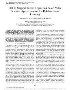
1 to state 2 with probability 1/2, to state 4 with probability 1/4, · · ·, to state 2k Pk+l−1 −i with probability 1/2k , etc. Let ωlk = 2 , and ²kl = 2−(k+l) and define i=1 ω ˆ k = (ω1k − ²k1 /2, ω2k − ²k2 /2, · · ·) and ω ˇ k = (ω1k + ²k1 /2, ω2k + ²k2 /2, · · ·). Thus, with noise sequence ω ˆ k , the transition from state 1 is to state x ˆ = 2k while with noise sequence ω ˇ k , the transition from state 1 is to state x ˇ = 2k+1 . Define the metric ρ on X × Ω∞ , ρ((x1 , ω ˆ k ), (x2 , ω ˇ k )) = |x1 − x2 | + |ˆ ω1 − ω ˇ 1 |. Then, it can be verified that ρ(f (1, ω ˆ k ), f (1, ω ˇ k )) = |ˆ x−x ˇ| + ²k2 ≥ 2k , ∀k, whereas Lipshitz continuity would require it be less that C2−(k+1) for some positive constant C and every k. Thus, f is not Lipschitz continuous on Ω∞ . (2) Consider the following Markov chain: State space X = N again endowed with the same metric ρ as in the above example. Transitions are deterministic: Transition from an even state n is to state 2n, and from an odd state n + 1 is to 3n. Then, ρ(f (n + 1, ω), f (n, ω)) = n and so is not Lipschitz continuous on X. These examples demonstrate that Lipschitz continuity of the simulation functions on a discrete state space is not the right assumption to make. 3. Markov games. The generalization of the results of this section to discountedreward Markov games is relatively straightforward. It is of considerable interest for many applications [38, 32]. Consider two players playing a Markov game with action spaces A1 and A2 , state space X, and transition function Pa1 ,a2 (x, y), a1 ∈ A1 , a2 ∈ A2 . We only consider stationary policy spaces Π1 and Π2 . The two reward functions r1 and r2 depend only on the state and have values in [0, R]. Denote the discounted reward functions by V1 (π1 , π2 ) and V2 (π1 , π2 ) with discount factor 0 < γ < 1. Denote the set of Markov chains induced Pby the policies in Π1 ×Π2 by P = {Pπ1 ,π2 : (π1 , π2 ) ∈ Π1 × Π2 )} with Pπ1 ,π2 (x, y) = a1 ,a2 Pa1 ,a2 (x, y)π1 (x, a1 )π2 (x, a2 ). Of interest is a uniform sample complexity bound such that the error in estimating both V1 (π1 , π2 ) and V2 (π1 , π2 ) is within ² with probability at least 1 − δ. This is now easily obtained by using theorem 5.2 and bounding the maximum of the estimation error in V1 and V2 . Such estimates may be used to compute the Nash equilibria [38]. A bound on the ²-covering number of P can be easily obtained by constructing ²/2-covers for Π1 and Π2 under the L1 metric and then the ² cover for Π1 × Π2 is obtained by taking the product of the two sets. The rest of the argument is the same as in Lemma 3.1. 4. We now show through two examples that which simulation model is used for generating the sample trajectories affects whether we get uniform convergence or not. Example 5.4. (i) Consider the three-state Markov chain with the following tranState 0

p

1-p

1

1 State -1

State 1

Fig. 5.1. A three state Markov chain with initial state 0.

12

JAIN AND VARAIYA

sition matrix 

0 P = 0 0

 p 1−p 1 0  0 1

and with state 0 always the initial state. Let P = {P as defined above with 0 ≤ p ≤ 1} denote the set of all such Markov chains as p varies. It is easy to check that P is convex and has P-dimension one. Let the reward in state 0 be 0, in state -1 be -1 and in state 1 be 1. This defines a Markov reward process and for a given p, we get the value Vp = 1 − 2p. Let F be the set of simple simulation functions that simulate the Markov chains in P. By lemma 4.2, P-dim(F) is one as well. Now, consider the following set of simulations functions. Fix p ∈ [0, 1]. Let x1 , x2 , · · · be rational numbers in [0, 1] such that (5.3)

0 ≤ x1 ≤ x1 + p/2 ≤ x2 ≤ x2 + p/4 · · · ≤ 1.

Generate a uniform [0, 1] random number ω. If it falls in [x1 , x1 + p/2] ∪ [x2 , x2 + p/4]∪· · · then the next state is -1, else 1. This simulation function simulates a Markov chain with parameter p. Let F˜ denote the set of all such simulation functions as p varies in [0, 1] and for every possible sequence of rational numbers satisfying (5.3). It ˜ is not finite. Now, consider any ω1 , ω2 , · · · ωn ∈ [0, 1]. is easy to check that P-dim(F) Then, there exists a p and x1 , x2 , · · · such that ωk ∈ [xk , xk + p/2k ] which means there is a simulation function which always goes to state -1 for this sequence of random numbers. Since n is arbitrary, this implies Vˆp = −1 6= Vp for some p. Thus, in this case, even though the second set of simulation functions F˜ simulate the same set of Markov chains P, we do not get uniform convergence. In the example above, there are many simulation functions in F that simulate the same Markov chain in P. We now modify the example so that there is only one simulation function for each Markov chain. (ii) Fix a positive integer m. Consider the [0, 1] interval divided into m2 subin¡ 2¢ tervals of length 1/m2 . Pick any m of these subintervals, which can be done in m m ways. Order these choices in any order. Define µ 2¶ 1 k 1 m pm,k = + ¡m2 ¢ ≤ , k = 1, · · · , . m+1 m m m m(m + 1) Scale the length of each of the m subintervals of the kth such choice to pm,k /m ≤ 1/m2 keeping the beginning point of the subintervals the same. Now, for every pm,k as de¡ 2¢ fined above with k = 1, · · · , m m and m = 1, 2, · · ·, define a simulation function fm,k such that for the Markov chain with parameter pm,k , if the current state is zero, and the uniform [0, 1] random number falls in any of the subintervals, then the next state is -1, else 1. All other Markov chains are simulated according to the simple simulation model. Thus, we get a new set of simulation functions F¯ with each Markov chain ¯ is being simulated by only one simulation function. It is easy to check that P-dim(F) not finite. Further, given any ω1 , ω2 , · · · , ωn ∈ [0, 1], we can always pick an m large enough such that there is a km so that all of the ωi lie outside the m subintervals, each of length pm,km /m. Thus, the simulation goes to state -1 for each of the ωi . Thus, Vˆpm,km 6= Vpm,km and we do not get uniform convergence.

UNIFORM ESTIMATION FOR MARKOV DECISION PROCESSES

13

These examples demonstrate that uniform convergence for MDPs depends not only on the geometry of the policy space but also on how the MDP is simulated to obtain the sample trajectories. The simple simulation model is in some sense the best model since it has the same complexity under convexity as the set of Markov chains it simulates (Lemma 4.2). However, note that these examples are note provided to emphasize the necessity of assumptions in theorem 5.2. Those are sufficient conditions only. An Alternative Simulation Method for Finite-dimensional Convex Spaces. An important special case is when the policy space is the convex hull of a finite number of policies, i.e., all policies are (random) mixtures of finitely many policies. While the previous simulation method would still work, we present an alternative simulation method that exploits the convex structure. The simulation method is the following. Suppose there are two policies πi for i = 0, 1, each inducing a Markov chain Pi with simulation function fi . Consider the mixture πw = wπ0 + (1 − w)π1 , so Pw = wP0 + (1 − w)P1 . For t steps, we have Pwt = wt P0t + wt−1 (1 − w)P0t−1 P1 + wt−1 (1 − w)P0t−2 P1 P0 + · · · + (1 − w)t P1t . Note that P0 and P1 need not commute. To obtain Vˆn (π), we first determine the rewards at time t for t = 0, · · · , T . To estimate the rewards, first draw the initial states x10 , · · · , xn0 from λ, and the noise sequences ω 1 , · · · , ω n from µ. Then carry out 2t simulations, one for each term in the sum of equation above. For example, if it · · · i1 is the binary representation of k then the contribution to reward from the kth term is determined by r ◦ fit ◦ · · · ◦ fi1 (xi0 , ω i ). The estimate of the contribution to reward ˆ tk is the mean over the n initial state and noise sequence pairs. from the kth term, R The estimate of the reward at time t is ˆ t2t −1 ˆ t0 + wt−1 (1 − w)R ˆ t1 + · · · + (1 − w)t R ˆ t = wt R R PT ˆ t . This can be generalized to a and the value function estimate Vˆn (π) is t=0 γ t R policy space which is a convex hull of any finite number of policies. Theorem 5.5. Let Π = conv{π0 , · · · , πd−1 }, P = conv{P0 , · · · , Pd−1 } the space of Markov chains induced by Π, and F the space of simulation functions of P under the simple simulation model. Let Vˆn (π), the estimate of V (π) obtained from n samples. Then, given any ², δ > 0 Pn {sup |Vˆn (π) − V (π)| > ²} < δ π∈Π

¡ ¢ R2 for n ≥ 2α log 1δ + T log 2d where T is the ²/2 horizon time and α = ²/2(T + 1). 2 Pd−1 Proof. Consider P any π ∈ Π andt the corresponding P ∈ P. Let P = i=0 ai Pi with ai ≥ 0 and i ai = 1. Thus, P can be written as (5.4)

t

P =

t dX −1

wkt Pit · · · Pi1

k=0

where it · · · i1 is a d-ary representation of k and the non-negative weights wkt are such Pdt −1 that k=0 wkt = 1 and can be determined easily. To obtain Vˆn (π), we need to simulate P for T steps as before. The t-step reward is determined by the state at time t, whose distribution is given by νt = P t λ. To

14

JAIN AND VARAIYA

estimate the reward, first draw the initial states x10 , · · · , xn0 from λ, and the noise sequence ω 1 , · · · , ω n from µ. We carry out dt simulations, one for each term in the sum of (5.4). Recall that it · · · i1 is a d-ary representation of k. Thus, to determine the contribution to the empirical reward at time t due to the kth term in (5.4), the state at time t is determined by r ◦ fit ◦ · · · ◦ fi1 (xi0 , ω i ). Thus, an estimate of the expected reward at time t is ˆ t (w ) = R t

(5.5)

t dX −1

à wkt

k=0

! n 1X i i r ◦ fit ◦ · · · ◦ fi1 (x0 , ω ) , n i=1

PT ˆ t (wt (π)), where a consistent estimator of EP t λ [r(x)]. Vˆn (π) is now given by t=0 γ t R t w (π) are the weights determined in equation 5.4 by policy π at time t. Denote Wt := {wt (π) : π ∈ Π}. Note that (5.6)

E

P tλ

[r(x)] =

t dX −1

¡ ¢ wkt EPit ···Pi1 λ [r(x)]

k=0

ˆ tk ) is an estimator for the where the quantity in the bracket of (5.5) (denote it by R quantity in the bracket of (5.6). Thus, ˆ t (wt ) − EP t λ [r(x)]| > α} Pn {sup |Vˆn (π) − V (π)| > ²} ≤ Pn { sup |R π∈Π

wt ∈Wt

ˆ tk − EP ···P λ [r(x)]| > α} ≤ dT max Pn {|R it i1 k

≤ 2dT exp(−

2nα2 ), R2

where α = ²/2(T + 1) and the last inequality follows from Hoeffdings inequality. From the above, the sample complexity can be obtained as in the proof of Theorem 5.2. Remarks. This alternative simulation model has the same order of sample complexity as in the earlier case, but it has greater computational complexity since for each chain, dT simulations need to be carried out. However, if several Markov chains need to be simulated, as when performing optimal policy search, the simulation is carried out only once for all the chains, because the estimates for various mixtures ˆ tk . are obtained by appropriately weighing the dt estimates, R Also, to obtain the estimates for t ≤ T , one need not repeat the simulation for each t. Instead, the T step simulation suffices to yield the t step estimate by simply ignoring the simulation beyond t + 1. Thus, only dT simulations are needed to obtain an estimate for reward for any step t ≤ T and any P ∈ P. 6. Average-reward MDPs. Some MDP problems use the average-reward criterion. However, there are no published results on simulation-based uniform estimates of value functions of average-reward MDPs. We present such a result in this section. Unlike the discounted-reward case, where we simulated several different sample paths, starting with different initial states, here the estimate is obtained from only one sample path. This is possible only when the policies we consider are such that the Markov chains are stationary, ergodic and weakly mixing. (The conditions under which a policy induces a stationary, ergodic Markov chain can be found in chapter 5 of [9].) A related problem is addressed in [22]. They use Csiszer’s concentration

UNIFORM ESTIMATION FOR MARKOV DECISION PROCESSES

15

inequality to bound reward functionals for Doeblin chains. However, the bound is not uniform and distribution dependent. Let λπ denote the invariant measure of the Markov chain {Xk }∞ k=0 with transition probability function Pπ , and Λ the set of all such invariant measures. Let P denote the probability measure for the process. We assume that there is a Markov chain P0 with invariant measure (steady state distribution) λ0 such that λπ ¿ λ0 , i.e., λπ is absolutely continuous w.r.t. λ0 meaning that λπ (A) = 0 if λ0 (A) = 0 for any measurable set A [18]. We call such a chain a reference Markov chain. Let ~π (x) := λπ (x)/λ0 (x) be the Radon-Nikodym derivative and assume that it is uniformly bounded, ~π (x) ≤ K for all x and π. Let H be the set of all such RadonNikodym derivatives. Our simulation methodology is to generate a sequence {xk }nk=1 according to P0 . We then multiply r(xt ) by ~π (xt ) to obtain the tth-step reward for the Markov chain induced by policy π. The estimate of the value function is then obtained by taking an empirical average of the rewards, i.e., n

1X Vˆn (π) = r˜π (xt ), n t=1 in which r˜π (x) := rπ (x)~π (x). Let R = {˜ rπ : π ∈ Π}. Furthermore, in some problems such as when the state space is multidimensional or complex, it may not be possible to integrate the reward function with respect to the stationary measure. In such cases, Monte Carlo type methods such as importance sampling are useful for estimating integrals. The method proposed here falls in such a category and we present a uniform rate of convergence result for it. This approach is useful when it is difficult to sample from the stationary distributions of the Markov chains but easy to compute the derivative ~π (x). We first state some definitions and results needed in the proof below. Let {Xn }∞ n=−∞ ∞ ergodic be a process on the measurable space (X∞ −∞ , S−∞ ). Consider a stationary,Q ¯ = ∞ P, process with measure P. Let P be the one-dimensional marginal, and P −∞ the product measure under which the process is i.i.d. Let P0−∞ and P∞ 1 be the semi-infinite marginals of P. Define the β-mixing coefficients [14] as 0 ∞ β(k) := sup{|P(A) − P0−∞ × P∞ 1 (A)| : A ∈ σ(X−∞ , Xk )}.

If β(k) → 0 as k → ∞, the process is said to be β-mixing (or weakly mixing). From the definition of the β-mixing coefficients we get ¯ Fact 1 ([29, 50]). If A ∈ σ(X0 , Xk , · · · , X(m−1)k ), |P(A) − P(A)| ≤ mβ(k). We assume that the Markov chain P0 is β-mixing with mixing coefficients β0 . We also need the following generalization of Hoeffding’s bound. Fact 2 (McDiarmid-Azuma inequality [5, 27]). Let X1 , · · · , Xn be i.i.d. drawn according to P and g : X n → R. Suppose g has bounded differences, i.e., |g(x1 , · · · , xi , · · · , xn ) − g(x1 , · · · , x0i , · · · , xn )| ≤ ci . Then, ∀τ > 0, 2τ 2 P n {g(X n ) − Eg(X n ) ≥ τ } ≤ exp(− Pn

2 ). i=1 ci

16

JAIN AND VARAIYA

We now show that the estimation procedure enunciated above for the average reward case produces estimates Vˆ (π) that converge uniformly over all policies to the true value V (π). Moreover, we can obtain the rate of convergence, whose explicit form depends on the specific problem. Theorem 6.1. Suppose the Markov chains induced by π ∈ Π are stationary and ergodic. Assume there exists a Markov chain P0 with invariant measure λ0 and mixing coefficient β0 such that λπ ¿ λ0 and the ~π are bounded by a constant K with P-dim (H) ≤ d. Denote by Vˆn (π), the estimate of V (π) from n samples. Then, given any ², δ > 0, P0 {sup |Vˆn (π) − V (π)| > ²} < δ, π∈Π

2

1 1/2 for n large enough such that γ(m) + Rmβ0 (k) + τ (n) ≤ ² where τ (n) := ( 2R n log δ ) and µ ¶d 32eRK mα2 32eRK γ(m) := inf {α + 8R log exp(− )}, α>0 α α 32R2

with n = mn kn such that mn → ∞ and kn → ∞ as n → ∞. Proof. The idea of the proof is to use the β-mixing property and reduce the problem to one with i.i.d. samples. We then use techniques similar to those used in the proof of Theorem 5.2. The problem of iteration of simulation functions does not occur in this case, which makes the proof easier. Let x1 , x2 , · · · , xn be the state sequence generated according to P0 which can be done using the simple simulation model. Note that E0 [r(x)~π (x)] = Eλπ [r(x)], in which Eλπ and E0 denote expectation taken with respect to the stationary measures Pn ˆ n [˜ λπ and λ0 respectively. Denote E rπ ; xn ] := n1 t=1 r˜π (xt ) and observe that X (1) 1 k−1

ˆ n [˜ E0 [sup |E rπ ; xn ] − E0 [˜ rπ (x)]|] ≤

k

π∈Π

j=0

E0 [sup | π∈Π

(2)

m−1 1 X r˜π (xlk+j ) − E0 [˜ rπ (x)]|] m

≤ α + RP0 {sup | π∈Π

l=0

1 m

m−1 X

r˜π (xlk ) − E0 [˜ rπ (x)]| > α}

l=0

(3)

≤ α + Rmβ0 (k) m−1 1 X ¯ r˜π (xlk ) − E0 [˜ rπ (x)]| > α}, +RP0 {sup | π∈Π m l=0

¯ 0 is the i.i.d. product measure in which E0 is expectation with respect to P0 and P corresponding to P0 . Inequality (1) follows by triangle inequality, (2) by stationarity and the fact that the reward function is bounded by R, and (3) by definition of the β-mixing coefficients. Claim 1. Suppose ~π (x) ≤ K for all x and π and that P-dim (H) ≤ d. Then, ∀α > 0 ¶d µ 2eRK 2eRK log . C(α, R, dL1 ) ≤ 2 α α

UNIFORM ESTIMATION FOR MARKOV DECISION PROCESSES

17

Proof. Let λ0 be a probability measure on X. Observe that for r˜1 , r˜2 ∈ R, X dL1 (λ0 ) (˜ r1 , r˜2 ) = |˜ r1 (x) − r˜2 (x)|λ0 (x) x

≤R·

X

|~1 (x) − ~2 (x)|λ0 (x)

x

= R · dL1 (λ0 ) (~1 , ~2 ). As argued for similar results earlier in the paper, this implies the desired conclusion. From Theorem 5.7 in [49], we then get m−1 X mα2 ¯ 0 {sup | 1 P r˜π (xlk ) − E0 [˜ rπ (x)]| > α} ≤ 4C(α/16, R, dL1 ) exp(− ) 32R2 π∈Π m l=0

≤ 8(

32eRK 32eRK d mα2 log ) exp(− ). α α 32R2

Substituting above, we get ˆ n [˜ E0 [sup |E rπ ; xn ] − E0 [˜ rπ (x)]|] ≤ γ(m) + Rmβ0 (k). π∈Π

Now, defining g(xn ) as the argument of E0 above and using the McDiarmidAzuma inequality with ci = R/n, we obtain that ˆ n [˜ P0 {sup |E rπ ; xn ] − E0 [˜ rπ (x)]| ≥ γ(m) + Rmβ0 (k) + τ (n)} < δ π∈Π

where δ = exp(−2nτ 2 (n)/R2 ) and hence the desired result. Note that by assumption of the mixing property, β0 (kn ) → 0, and for fixed ² and δ, γ(mn ), τ (n) → 0 as n → ∞. The sample complexity result is implicit here since given functions γ, β0 and τ , we can determine n, mn and kn such that n = mn kn , mn → ∞, kn → ∞ and γ(mn ) + Rmn β0 (kn ) + τ ≤ ² for given ² and δ. The existence of mn and kn sequences such that mn β(kn ) → 0 is guaranteed by Lemma 3.1 in [49]. This implies δ → 0 as n → ∞ and thus the policy space Π is PAC-learnable under the hypothesis of the theorem. One of the assumptions we have made is that for policy π, the Radon-Nikodym derivative ~π is bounded by K. This essentially means that all the Markov chains are close to the reference Markov chain in the sense that the probability mass on any state does not differ by more than a multiplicative factor of K from that of P0 . The assumption that H has finite P-dimension is less natural but essential to the argument. Let us now show the existence of reference Markov chains through an example. Example 6.2. Consider any Markov chain with invariant measure P λ0 . Consider any parametrized class of functions ~π : X → [0, 1], π ∈ Π such that x λ0 (x)~π (x) = 1 and P-dim({~π : π ∈ Π}) = d. Denote λπ (x) = λ0 (x)~π (x) and consider a set of Markov chains P with invariant measures λπ . Then, clearly, λ0 is an invariant measure of a reference Markov chain for the set P of Markov chains. 7. Partially Observable MDPs with General Policies. We now consider partially observed discounted-reward MDPs with general policies (non-stationary with memory). The setup is as before, except that the policy depends on observations

18

JAIN AND VARAIYA

y ∈ Y, governed by the (conditional) probability ν(y|x) of observing y ∈ Y when the state is x ∈ X. Let ht denote the history (y0 , a1 , y1 , · · · , at , yt ) of observations and actions up to time t. The results of section 5 extend when the policies are non-stationary however there are many subtleties regarding the domain and range of simulation functions, and measures, and some details are different. Let Ht = {ht = (y0 , a1 , y1 , · · · , at , yt ) : as ∈ A, ys ∈ Y, 0 ≤ s ≤ t}. Let Π be the set of policies π = (π1 , π2 , · · ·), with πt : Ht × A → [0, 1] a probability measure on A conditioned on ht ∈ Ht . Let Πt denote the set of all policies πt at time t with π ∈ Π. This gives rise to a conditional state transition function Pt (x, x0 ; ht ), the probability of transition from state x to x0 given history ht up to time t. Under π, X Pa (x, x0 )πt (ht , a). Pt (x, x0 ; ht ) = a

Let Pt denote the set of all Pπt induced by the policies πt with π ∈ Π. Then, defining the usual dT V (λ) metric on Pt and the usual L1 metric on Πt , we get the next result. Lemma 7.1. Suppose Πt and Pt are as defined above with P-dim (Πt ) = d. Assume λ and ρ are probability measures on X and Ht respectively, and σ a probability measure on A such that πt (ht , a)/σ(a) ≤ K, ∀ht ∈ Ht , a ∈ A, πt ∈ Πt . Then, for 0 < ² < e/4 log2 e, µ ¶d 2eK 2eK N (², Pt , dT V (λ×ρ) ) ≤ N (², Πt /σ, dL1 (σ×ρ) ) ≤ log . ² ² The proof can be found in the appendix. Let Ft be the set of simulation functions of Pt under the simple simulation model. Thus, a ft ∈ Ft for t ≥ 2 is defined on ft : X × Ht−1 × Ω∞ → X × Ht × Ω∞ while f1 ∈ F1 shall be defined on f1 : X × Ω∞ → X × H1 × Ω∞ . This is because at time t = 1, there is no history, and the state transition only depends on the initial state and the noise. For t > 1, the state transition depends on the history as well. Further, the function definitions have to be such that the composition ft ◦ ft−1 ◦ · · · ◦ f1 is well-defined. It is straightforward to verify that Lemma 4.2 extends. Lemma 7.2. Suppose P is convex (being generated by a convex space of policies Π). Let P-dim (Pt ) = d. Let Ft be the corresponding space of simple simulation functions induced by Pt . Then, P-dim (Ft ) = d. By F t we shall denote the set of functions f t = ft ◦· · ·◦f1 where fs ∈ Fs and they arise from a common policy π. Note that f t : X × Ω∞ → Zt × Ω∞ where Zt = X × Ht . We shall consider the following pseudo-metric on Ft with respect to a measure λt on Zt−1 for t ≥ 2 and measure σ on Ω∞ , X ρt (ft , gt ) := λt (z)σ{ω : ft (z, ω) 6= gt (z, ω)}. z∈Zt−1

We shall take ρ1 as the pseudo-metric on F t w.r.t the product measure λ × σ. Let X λf t (z) := λ(x)σ{ω : f t (x, ω) = (z, θt ω)} z∈Zt

be a probability measure on Zt . We now state the extension of the technical lemma needed for the main theorem of this section.

19

UNIFORM ESTIMATION FOR MARKOV DECISION PROCESSES

Lemma 7.3. Let λ be a probability measure on X and λf t be the probability measure on Zt as defined above. Suppose that P-dim (Ft ) ≤ d and there exists probability λf t (z) measures λt on Zt such that K := max{supt supf t ∈F t ,z∈Zt λt+1 (z) , 1} < ∞. Then, for 1 ≤ t ≤ T , ² ² N (², F , ρ1 ) ≤ N ( , F t , ρt ) · · · N ( , F1 , ρ1 ) ≤ Kt Kt t

µ

2eKt 2eKt log ² ²

¶dt .

The proof can be found in the appendix. We now obtain our sample complexity result. Theorem 7.4. Let (X, Γ, λ) be the measurable state space, A the action space, Y the observation space, Pa (x, x0 ) the state transition function and ν(y|x) the conditional probability measure that determines the observations. Let r(x) the real-valued reward function bounded in [0, R]. Let Π be the set of stochastic policies (non-stationary and with memory in general), Pt be the set of state transition functions induced by Πt , and Ft the set of simulation functions of Pt under the simple simulation model. Suppose that P-dim (Pt ) ≤ d. Let λ and σ be probability measures on X and A respectively and λf t (z) λt+1 a probability measure on Zt such that K := max{supt supf t ∈F t ,z∈Zt λt+1 (z) , 1} is finite, where λf t is as defined above. Let Vˆn (π), the estimate of V (π) obtained from n samples. Then, given any ², δ > 0, and with probability at least 1 − δ, sup |Vˆn (π) − V (π)| < ²

π∈Π

¢ 2 ¡ log 4δ + 2dT (log 32eR for n ≥ 32R α2 α + log KT ) where T is the ²/2 horizon time and α = ²/2(T + 1). Remarks. A special case is when the policies are stationary and memoryless, i.e., πt = π1 for all t, and π1 : Y × A → [0, 1] depends only on the current observation. Let Π1 be the set of all π1 . Then, each policy π ∈ Π induces a timehomogeneous Markov chain with probability transition function given by Pπ (x, x0 ) = P 0 a,y Pa (x, x )π1 (y, a)ν(y|x). Let P denote the set of all probability transition functions induced by Π. In general if Π is convex, P is convex. We will denote the set of simulation functions under the simple simulation model for P ∈ P by F. Suppose that P-dim (P) = d, then by Lemma 4.2, P-dim (P) = P-dim (F) = d. This implies that the sample complexity result of Theorem 5.2 for discounted-reward MDPs holds for the case when the state is partially observable and the policies are stationary and memoryless. Thus, for uniform convergence and estimation, partial observability of the state does not impose any extra cost in terms of sample complexity. Note that in the case of general polices, the sample complexity is O(T log T ) times more. 8. Conclusions. The paper considers simulation-based value function estimation methods for Markov decision processes (MDP). Uniform sample complexity results are presented for the discounted reward case. The combinatorial complexity of the space of simulation functions under the proposed simple simulation model is shown to be the same as that of the underlying space of induced Markov chains when the latter is convex. Using ergodicity and weak mixing leads to similar uniform sample complexity result for the average reward case, when a reference Markov chain exists. Extension of the results are obtained when the MDP is partially observable with general policies. Remarkably, the sample complexity results have the same order for both completely and partially observed MDPs when stationary and memoryless

20

JAIN AND VARAIYA

policies are used. Sample results for discounted-reward Markov games can be deduced easily as well. The results can be seen as an extension of the theory of PAC (probably approximately correct) learning for partially observable Markov decision processes (POMDPs) and games. PAC theory is related to the the system identification problem. One of the key contributions of this paper is the observation that how we simulate an MDP matters for obtaining uniform estimates. This is a new (and suprising) observation. Thus, the results of this paper can also be seen as the first steps towards developing an empirical process theory for Markov decision processes. Such a theory would go a long way in establishing a theoretical foundation for computer simulation of complex engineering systems. We have used Hoeffding’s inequality in obtaining the rate of convergence for discounted-reward MDPs and the McDiarmid-Azuma inequality for the average-reward MDPs, though more sophisticated and tighter inequalities of Talagrand [37, 41] can be used as well. This would yield better results and is part of future work. Acknowledgments. We thank Peter Bartlett, Tunc Simsek and Antonis Dimakis for many helpful discussions. The counterexample 5.4(ii) was jointly developed with Antonis Dimakis. We also thank the anonymous referees for their comments which helped to greatly improve the quality of the paper. Appendix A. Proof of Lemma 3.1. Proof. We first relate the dT V (λ) pseudo-metric on P with the dL1 (λ×σ) pseudometric on Π. Pick any π, π 0 ∈ Π and denote P = Pπ , and P 0 = Pπ0 . Then, X X X dT V (λ) (P, P 0 ) = | λ(x) Pa (x, y)(π(x, a) − π 0 (x, a))| y

≤

a

≤

x

XXX X a

x

σ(a)

a

λ(x)Pa (x, y)|π(x, a) − π 0 (x, a)|

y

X

λ(x)|π(x, a) − π 0 (x, a)|/σ(a)

x

= dL1 (σ×λ) (π/σ, π 0 /σ). The second inequality above follows from the triangle inequality and the fact that the orderP of the sums over y, x and a can be changed by Fubini’s theorem [18] and noting that y Pa (x, y) = 1. Thus, if Π0 /σ ⊆ Π/σ is an ²-net for Π/σ, {Pπ , π ∈ Π0 } is an ²-net for P. Further, the space Π and Π/σ have the same P-dimension, as can be easily verified. The bound on the covering number is then given by a standard result (see Theorem 4.3, [49]). Appendix B. Proof of Lemma 5.1. Proof. Consider any f, g ∈ F and x ∈ X . Then, µ{ω : f t (x, ω) 6= g t (x, ω)} = µ{ω : f t (x, ω) 6= g t (x, ω), f t−1 (x, ω) = g t−1 (x, ω)} +µ{ω : f t (x, ω) 6= g t (x, ω), f t−1 (x, ω) 6= g t−1 (x, ω)} = µ{∪y (ω : f t (x, ω) 6= g t (x, ω), f t−1 (x, ω) = g t−1 (x, ω) = (y, θt−1 ω))} +µ{∪y (ω : f t (x, ω) 6= g t (x, ω), f t−1 (x, ω) 6= g t−1 (x, ω), f t−1 (x, ω) = (y, θt−1 ω))} ≤ µ{∪y (ω : f (y, θt−1 ω) 6= g(y, θt−1 ω), f t−1 (x, ω) = g t−1 (x, ω) = (y, θt−1 ω))} +µ{∪y (ω : f t−1 (x, ω) 6= g t−1 (x, ω), f t−1 (x, ω) = (y, θt−1 ω))}

UNIFORM ESTIMATION FOR MARKOV DECISION PROCESSES

≤

X

21

µ{ω : f (y, θt−1 ω) 6= g(y, θt−1 ω)|f t−1 (x, ω) = (y, θt−1 ω)}µ{ω : f t−1 (x, ω) = y}

y

+µ{ω : f t−1 (x, ω) 6= g t−1 (x, ω)}. P It is easy to argue that λf t−1 (y) ≤ K t−1 λ(y) where λf t−1 (y) = x λ(x)µ{ω : f t−1 (x, ω) = (y, θt−1 ω)}. Thus, multiplying both RHS and LHS of the above sequence of inequalities and summing over x, and observing that µ{ω : f (y, θt−1 ω) 6= g(y, θt−1 ω)} = µ{ω 0 : f (y, ω 0 ) 6= g(y, ω 0 )} we get that the first part of RHS is X X λf t−1 (y)µ{ω 0 : f (y, ω 0 ) 6= g(y, ω 0 )} ≤ K t−1 · λ(y)µ{ω 0 : f (y, ω 0 ) 6= g(y, ω 0 )} y

y

This implies that ρP (f t , g t ) ≤ K t−1 ρP (f, g) + ρP (f t−1 , g t−1 ) ≤ (K t−1 + K t−2 + · · · + 1)ρP (f, g) ≤ K t ρP (f, g). where the second inequality is obtained by induction. Now, Z X X λ(x)µ{ω : f (x, ω) 6= g(x, ω)} ≤ λ(x) |f (x, ω) − g(x, ω)|dµ(ω) x

x

and thus ρP (f t , g t ) ≤ K t · dL1 (f, g) which proves the required assertion. Appendix C. Proof of Lemma 7.1. Proof. Pick any πt , πt0 ∈ Πt , and denote P = Pπt and P 0 = Pπt0 . Then, dT V (λ×ρ) (P, P 0 ) =

X x

≤

X

X

λ(x)

≤

X

Pa (x, x0 )(πt (ht , a) − πt0 (ht , a))|ρ(ht )

x0 ∈X a∈A,ht ∈Ht

ρ(ht )

X

λ(x)

XX

x

ht

X

|

ρ(ht )

X

ht

= dL1 (σ×ρ) (

a

σ(a)|

a

Pa (x, x0 )|πt (ht , a) − πt0 (ht , a)|

x0

πt (y, a) πt0 (y, a) − | σ(a) σ(a)

πt πt0 , ). σ σ

0 The second inequality above follows by changing P P the order of the sums over a and x , 0 noting that x0 Pa (x, x ) = 1 and denoting x λ(x) = 1. The rest of the argument is the same as in Lemma 3.1.

Appendix D. Proof of Lemma 7.3. The proof of Lemma 7.3 is similar but the details are somewhat more involved. Proof. Consider any f t , g t ∈ F t and x ∈ X . Then, µ{ω : f t (x, ω) 6= g t (x, ω)} = µ{ω : f t (x, ω) 6= g t (x, ω), f t−1 (x, ω) = g t−1 (x, ω)}

22

JAIN AND VARAIYA

+µ{ω : f t (x, ω) 6= g t (x, ω), f t−1 (x, ω) 6= g t−1 (x, ω)} = µ{∪z∈Zt−1 (ω : f t (x, ω) 6= g t (x, ω), f t−1 (x, ω) = g t−1 (x, ω) = (z, θt−1 ω))} +µ{∪z∈Zt−1 (ω : f t (x, ω) 6= g t (x, ω), f t−1 (x, ω) 6= g t−1 (x, ω), f t−1 (x, ω) = (z, θt−1 ω))} ≤ µ{∪z∈Zt−1 (ω : f t (x, ω) 6= g t (x, ω), f t−1 (x, ω) = g t−1 (x, ω) = (z, θt−1 ω))} +µ{∪z∈Zt−1 (ω : f t−1 (x, ω) 6= g t−1 (x, ω), f t−1 (x, ω) = (z, θt−1 ω))} X ≤ µ{ω : ft (z, θt−1 ω) 6= gt (z, θt−1 ω)|f t−1 (x, ω) = (z, θt−1 ω)}µ{ω : f t−1 (x, ω) = (z, θt−1 ω)} z∈Zt−1

+µ{ω : f t−1 (x, ω) 6= g t−1 (x, ω)}.

Multiplying both RHS and LHS of the above sequence of inequalities and summing over x, and observing again that µ{ω : ft (z, θt−1 ω) 6= gt (z, θt−1 ω)} = µ{ω 0 : ft (z, ω 0 ) 6= gt (z, ω 0 )} we get that the first part of RHS is X X λf t−1 (z)µ{ω 0 : ft (z, ω 0 ) 6= gt (z, ω 0 )} ≤ K· λt (z)µ{ω 0 : ft (z, ω 0 ) 6= gt (z, ω 0 )}. z∈Zt−1

z∈Zt−1

This by induction implies ρ1 (f t , g t ) ≤ K(ρt (ft , gt ) + · · · + ρ1 (f1 , g1 )), which implies the first inequality. For the second inequality, note that the ρ pseudometric and the L1 pseudo-metric are related thus Z X X λt (z)µ{ω : ft (z, ω) 6= gt (z, ω)} ≤ λt (z) |ft (z, ω) − gt (z, ω)|dµ(ω). z

z

which relates their covering numbers. And the covering number under the L1 pseudometric can be bounded in terms of the P-dim of appropriate spaces. REFERENCES [1] D. Aldous and U. Vazirani, “A Markovian extension of Valiant’s learning model”, Information and computation, 117(2):181-186, 1995. [2] N. Alon, S. Ben-David, N. Cesa-Bianchi and D. Haussler, “Scale-sensitive dimension, uniform convergence and learnability”, J. of ACM, 44:615-631, 1997. [3] M. Anthony and P. Bartlett, Neural Network Learning: Theoretical Foundations, Cambridge University Press, 1999. [4] E. Altman and O. Zeitouni, “Rate of convergence of empirical measures and costs in controlled Markov chains and transient optimality”, Math. of Operations Research, 19(4):955974, 1994. [5] K. Azuma, “Weighted sums of certain dependent random variables”, Tohoku Mathematical J. , 68:357-367, 1967. [6] J. Baxtar and P. L. Bartlett, “Infinite-horizon policy-gradient estimation”, J. of A. I. Research, 15:319-350, 2001. [7] G. M. Benedek and A. Itai, “Learning with respect to fixed distributions”, Theoretical Computer Science, 86(2):377-390, 1991. [8] V. Bentkus, “On Hoeffding’s inequalities”, The Annals of Probability, 32(2):1650-1673, 2004. [9] V. Borkar, Topics in optimal control of Markov chains, Pitman Research Notes in Mathematics, 1991.

UNIFORM ESTIMATION FOR MARKOV DECISION PROCESSES

23

[10] M. C. Campi and P. R. Kumar, “Learning dynamical systems in a stationary environment”, Systems and Control Letters, 34:125-132, 1998. [11] H. Chernoff, “A measure of asymptotic efficiency of tests of a hypothesis based on the sum of observations”, Annals of Mathematical Statistics, 23:493-507, 1952. [12] L. Devroye, L. Gyorfi and G. Lugosi, A Probabilistic Theory of Pattern Recognition, Springer-Verlag, 1996. [13] P. Diaconis and D. Freedman, “Iterated random functions”, SIAM Review, 41(1):45-76, 1999. [14] P. Doukhan, Mixing: Properties and Examples, Lecture Notes in Statistics, 85, Springer-Verlag, Berlin, 1994. [15] R. Dudley, Uniform Central Limit Theorems, Cambridge University Press, 1999. [16] D. Gamarnik, “Extensions of the PAC framework to finite and countable Markov chains”, IEEE Trans. Information Theory, 49(1):338-345, 2003. [17] D. Haussler, “Decision theoretic generalizations of the PAC model for neural nets and other learning applications”, Information and Computation, 100(1):78-150, 1992. [18] P. R. Halmos, Measure Theory, Springer-Verlag, 1974. [19] W. Hoeffding, “Probability inequalities for sums of bounded random variables”, J. of the American Statistical Assoc. , 58:13-30, 1963. [20] M. Kearns, Y. Mansour and A. Y. Ng, “Approximate planning in large POMDPs via reusable trajectories”, Proc. Neural Information Processing Systems Conf. , 1999. [21] A. N. Kolmogorov and V. M. Tihomirov, “²-entropy and ²-capacity of sets in functional spaces”, American Math. Soc. Translation Series 2, 17:277-364, 1961. [22] I. Kontoyiannis, L.A. L.-Montano and S.P. Meyn, “Relative entropy and exponential deviation bounds for general Markov chains”, Proc. Int. Symp. on Inform. Theory, 2005. [23] M. Ledoux, The Concentration of Measure Phenomenon, Mathematical Surveys and Monographs, Volume 89, American Mathematical Soc. , 2001. [24] S. Mannor and J.N. Tsitsiklis, “On the empirical state-action frequencies in Markov decision processes under general policies”, to appear, Math. of Operations Research, 2005. [25] P. Marbach and J. N. Tsitsiklis, “Approximate gradient methods in policy-space optimization of Markov reward processes”, J. Discrete Event Dynamical Systems, Vol. 13:111-148, 2003. [26] K. Marton, “Measure concentration for Euclidean distance in the case of dependent random variables”, The Annals of Probability, 32(3B):2526-2544, 2004. [27] C. McDiarmid, “On the method of bounded differences”, In Surveys in Combinatorics 1989:148-188, Cambridge University Press, 1989. [28] P. Massart “Some applications of concentration inequalities to statistics”, Annales de la facult des sciences de l’universit de Toulouse, Mathmatiques, vol. IX, No. 2:245-303, 2000. [29] A. Nobel and A. Dembo, “A note on uniform laws of averages for dependent processes”, Statistics and Probability Letters, 17:169-172, 1993. [30] A. Y. Ng and M. I. Jordan, “Pegasus: A policy search method for large MDPs and POMDPs”, Proc. UAI, 2000. [31] C. H. Papadimitriou and J. N. Tsitsiklis, “The complexity of Markov decision processses”, Mathematics of Operations Research, 12(3):441-450, 1987. [32] M. Pesendorfer and P. S-Dengler, “Identification and estimation of dynamic games”, National Bureau of Economic Research Working Paper Series 9726, 2003. [33] L. Peshkin and S. Mukherjee, “Bounds on sample size for policy evaluation in Markov environments”, Lecture Notes in Computer Science, 2111:616-630, 2001. [34] D. Pollard, Convergence of Stochastic Processes, Springer-Verlag, Berlin, 1984. [35] D. Pollard, Empirical Process Theory and Applications, Institute of Mathematical Statistics, Hayward, CA, 1990. [36] M. Puterman, Markov decision processes: discrete stochastic dynamic programming, John Wiley and Sons, 1994. [37] P-M. Samson, “Concentration of measure inequalities for Markov chains for Φ-mixing processes”, The Annals of Probability, 28(1):416-461, 2000. [38] D. H. Shim, H. J. Kim and S. Sastry. “Decentralized nonlinear model predictive control of multiple flying robots in dynamic environments”, Proc. IEEE Conf. on Decision and Control, 2003. [39] J. M. Steele, Probability Theory and Combinatorial Optimization, SIAM, Philadelphia, PA, 1996. [40] M. Talagrand, “Concentration of measure and isoperimetric inequalities in product spaces”, Pub. Math. de l’I. H. E. S. , 81:73-205, 1995. [41] M. Talagrand, “A new look at independence”, The Annals of Probability, 24:1-34, 1996. [42] L. Valiant, “A theory of the learnable”, Communications of the ACM, 27(4):1134-1142, 1984.

24

JAIN AND VARAIYA

[43] S. Van de Geer, “On Hoeffding’s inequality for dependent random variables”, In Empirical Process Techniques for Dependent Data, eds. H. Dehling, T. Mikosch and M. Sorensen:161170, Birkhauser, Boston, 2002. [44] A. W. van der Vaart and J. A. Wellner, Weak Convergence and Empirical Processes, Springer-Verlag, Berlin, 1996. [45] V. Vapnik and A. Chervonenkis, “On the uniform convergence of relative frequencies to their empirical probabilities”, Theory of Probability and Applications, 16(2):264-280, 1971. [46] V. Vapnik and A. Chervonenkis, “Necessary and sufficient conditions for convergence of means to their expectations“, Theory of Probability and Applications, 26(3):532-553, 1981. [47] V. Vapnik and A. Chervonenkis, “The necessary and sufficient conditions for consistency in the empirical risk minimization method“, Pattern Recognition and Image Analysis, 1(3):283305, 1991. [48] M. Vidyasagar and R. L. Karandikar, “System identification: A learning theory approach”, Proceedings of the 40th IEEE Conference on Decision and Control, 2001. [49] M. Vidyasagar, Learning and Generalization: With Applications to Neural Networks, Second edition, Springer-Verlag, 2003. [50] B. Yu, “Rates of convergence of empirical processes for mixing sequences”, Annals of Probability, 22(1):94-116, 1994.