variety of linear function approximation schemes for con- tinuous domains, most commonly Radial Basis Functions. (RBFs) and CMACs (Sutton & Barto, 1998).
Value Function Approximation using the Fourier Basis
George Konidaris GDK @ CS . UMASS . EDU Sarah Osentoski SOSENTOS @ CS . UMASS . EDU Autonomous Learning Laboratory, Computer Science Dept., University of Massachusetts Amherst, 01003 USA
1. Introduction Reinforcement learning researchers have employed a wide variety of linear function approximation schemes for continuous domains, most commonly Radial Basis Functions (RBFs) and CMACs (Sutton & Barto, 1998). For most problems, choosing the right basis function set is criticial for successful learning. Unfortunately, most approaches require significant design effort or problem insight, and no basis function set is both sufficiently simple and sufficiently reliable to be generally satisfactory. Recent work (Mahadevan, 2005) has focused on learning basis function sets from experience, removing the need to design a function approximator but introducing the need to gather data to create one before learning can take place. In the applied sciences the most common continuous function approximation method is the Fourier Series. Although the Fourier Series is a simple and effective function approximator with solid theoretical underpinnings, it is almost never used in for value function approximation. We describe the Fourier Basis, a simple fixed linear function approximation scheme using the terms of the Fourier Series as basis functions. We present empirical results showing that it performs well compared to RBFs and the Polynomial Basis, and is competitive with Proto-Value Functions.
Although the Fourier Basis seems like a natural choice for value function approximation, we know of very few instances (e.g., (Kolter & Ng, 2007)) of its use in reinforcement learning, and no empirical study of its properties.
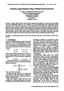
3. Empirical Evaluation 3.1. The Swing-Up Acrobot In the swing-up Acrobot (Sutton & Barto, 1998), we employed Sarsa(λ) (γ = 1.0, λ = 0.9, � = 0) for Fourier Bases of orders 3 (resulting in 256 basis functions), 5 (resulting in 1296 basis functions) and 7 (resulting in 4096 basis functions) and RBF, Polynomial and (normalized Laplacian) PVF bases of equivalent sizes. (We did not run PVFs with 4096 basis functions because the nearest-neighbour calculations for a graph that size proved too expensive) We systematically varied α (the gradient descent term) to obtain the best performance for each basis function type and order combination. The results (Figure 1) demonstrate that the Fourier Basis learners outperformed all other types of learning agents for all sizes of function approximators. In particular, the Fourier Basis performs better initially than the Polynomial Basis (which generalizes broadly) and converges to a better policy than the RBF Basis (which generalizes locally). It also performs slightly better than PVFs, even though the Fourier Basis is a fixed, rather than learned, basis.
2. The Fourier Basis 3.2. The Discontinuous Room
We define the univariate kth order Fourier Basis as: φi (x) = cos(iπx),
(1)
for i = 0, ..., k, and the kth order multivariate Fourier Basis for m variables as: φi (x) = cos(πci · x), i
(2)
where c = [c1 , ..., cm ], cj ∈ [0, ..., k], 0 ≤ j ≤ m is a coefficient vector which assigns integer weight cj for each input variable xj . The full basis includes terms for all such weight vectors (resulting in (k + 1)n terms for n input variables), although prior knowledge of the domain can be used to rule some out.
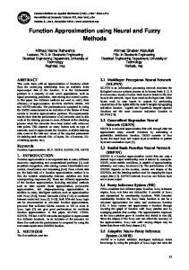
In the Discontinuous Room, show in Figure 2, an agent in a room must reach a target; however the direct path to the target is blocked by a wall, which the agent must go around. This domain is intended as a simple continuous domain with a large discontinuity, to empirically determine how the Fourier Basis handles such a discontinuity compared to Proto Value Functions, which were specifically designed to handle discontinuities. In order to make a reliable comparison, agents using PVFs were given a perfect adjacency matrix containing every legal state and transition, thus avoiding sampling issues and
The Fourier Basis 1400
1100
1400 O(3) Fourier 4 RBFs 16 PVFs
O(5) Fourier 1200
6 RBFs
1200
1200
O(5) Polynomial O(3) Fourier 4 RBFs O(3) Polynomial 256 PVFs
1000
900
1296 PVFs 1000
800
1000 800
700
Steps
Steps
800 Steps
800 Steps
6 RBFs O(5) Fourier 36 PVFs
1000
600 600
600
600 500
400
400
400
400 200
200
300 200
0
0 0
2
4
6
8
10 12 Episodes
14
16
18
20
200 0
5
10 Episodes
(a)
15
20 0
(b)
0
5
10 Episodes
(a)
15
20
100
0
5
10 Episodes
15
20
(b)
1000 O(7) Fourier 8 RBFs O(7) Polynomial
900 800
Figure 3. Learning curves for agents using (a) order 3 (b) order 5 Fourier Bases, and RBFs and PVFs with corresponding number of basis functions.
700
Steps
600 500 400 300 200 100 0
0
2
4
6
8
10 12 Episodes
14
16
18
20
(c) Figure 1. Learning curves for agents using (a) order 3 (b) order 5 and (c) order 7 Fourier Bases, and RBFs and PVFs with corresponding number of basis functions.
the Fourer Basis outperforms RBFs and PVFs. For higher orders, we see a repetition of the learning curve in Figure 2, where the Fourier Basis initially performs worse (because it does not model the discontinuity in the value function well) but converges to a better solution.
4. Summary 1000
Our results show that the Fourier Basis provides a simple and reliable basis for value function approximation. We expect that for many smaller problems, the Fourier Basis will be sufficient to learn a good value function without any extra work.
800 600
Reward
400 200 0 −200 36 PVFs −400
64 PVFs O(5) Fourier
−600 −800
O(7) Fourier 0
10
20
30
40
50 60 Episodes
70
80
90
100
Figure 2. The Discontinuous Room and its learning curves for agents using O(5) and O(7) Fourier Bases and agents using 36 and 64 PVFs.
removing the need for an out-of-sample extension method. We used Sarsa(λ) (γ = 0.9, λ = 0.9, � = 0) using Fourier Bases of order 5 and 7 and agents using 36 and 64 PVFs. The agents using the Fourier Basis do not initially perform as well as the agents using PVFs, probably because of the discontinuity, but this effect is transient and the Fourier Basis agents eventually perform better. 3.3. Mountain Car For Mountain Car (Sutton & Barto, 1998), we employed Sarsa(λ) (γ = 1.0, λ = 0.9, � = 0), Fourier Bases of orders 3 and 5, and RBFs and PVFs of equivalent sizes (we were unable to learn with the Polynomial Basis). Here we found it best to scale the α values for the Fourier Basis 1 , where m was the maximum degree of the basis by 1+m function. This allocated lower learning rates to higher frequency basis functions. The results (shown in Figure 3) indicate that for low orders,
Our experiences with the Fourier Basis show that it is a simple and easy to use basis set that reliably performs well on a range of different problems. As such, although it may not perform well for domains with several significant discontinuities, its simplicity and reliability suggest that the Fourier Basis should be the first function approximator used when reinforcement learning is applied to a new continuous problem. For the full version of this paper, please see Konidaris and Osentoski (2008).
References Kolter, J., & Ng, A. (2007). Learning omnidirectional path following using dimensionality reduction. Proceedings of Robotics: Science and Systems. Konidaris, G., & Osentoski, S. (2008). Value function approximation in reinforcement learning using the fourier basis (Technical Report UM-CS-2008-19). Department of Computer Science, University of Massachusetts, Amherst. Mahadevan, S. (2005). Proto-value functions: Developmental reinforcement learning. Proceedings of the Twenty Second International Conference on Machine Learning. Sutton, R., & Barto, A. (1998). Reinforcement learning: An introduction. Cambridge, MA: MIT Press.