Simulation Experiment Description Markup Language ...

Journal of Integrative Bioinformatics, 12(2):262, 2015

http://journal.imbio.de/

Simulation Experiment Description Markup Language (SED-ML) Level 1 Version 2

1

Department Modeling of Biological Processes, University of Heidelberg, Heidelberg, Germany 2

Department of Computer Science, University of Oxford, UK 3

4

5

6

The Babraham Institute, Cambridge, UK

EMBL European Bioinformatics Institute, Cambridge, UK

Auckland Bioengineering Institute, University of Auckland, Auckland, New Zealand

Department of Systems Biology and Bioinformatics, University of Rostock, Rostock, Germany Summary The number, size and complexity of computational models of biological systems are growing at an ever increasing pace. It is imperative to build on existing studies by reusing and adapting existing models and parts thereof. The description of the structure of models is not sufficient to enable the reproduction of simulation results. One also needs to describe the procedures the models are subjected to, as recommended by the Minimum Information About a Simulation Experiment (MIASE) guidelines. This document presents Level 1 Version 2 of the Simulation Experiment Description Markup Language (SED-ML), a computer-readable format for encoding simulation and analysis experiments to apply to computational models. SED-ML files are encoded in the Extensible Markup Language (XML) and can be used in conjunction with any XML-based model encoding format, such as CellML or SBML. A SED-ML file includes details of which models to use, how to modify them prior to executing a simulation, which simulation and analysis procedures to apply, which results to extract and how to present them. Level 1 Version 2 extends the format by allowing the encoding of repeated and chained procedures.

* To

whom correspondence should be addressed. Email: [email protected]

doi:10.2390/biecoll-jib-2015-262

Unauthenticated1 Download Date | 12/8/17 3:34 AM

Copyright 2015 The Author(s). Published by Journal of Integrative Bioinformatics. This article is licensed under a Creative Commons Attribution-NonCommercial-NoDerivs 3.0 Unported License (http://creativecommons.org/licenses/by-nc-nd/3.0/).

` 3,4 , David Nickerson5 and Frank T. Bergmann1 , Jonathan Cooper2* , Nicolas Le Novere 6 Dagmar Waltemath


http://journal.imbio.de

December 2, 2013

Editors

Frank T. Bergmann Jonathan Cooper Nicolas Le Novère David Nickerson Dagmar Waltemath

University of Washington, Seattle, USA University of Oxford, UK European Bioinformatics Institute, UK Auckland Bioengineering Institute, New Zealand University of Rostock, Germany

The latest release of the Level 1 Version 2 specification is available at http://identifiers.org/combine.specifications/sed-ml.level-1.version-2 To discuss any aspect of the current SED-ML specification as well as language details, please send your messages to the mailing list [email protected]. To get subscribed to the mailing list, please write to the same address [email protected]. To contact the authors of the SED-ML specification, please write to [email protected]


Unauthenticated Download Date | 12/8/17 3:34 AM


Simulation Experiment Description Markup Language (SED-ML) : Level 1 Version 2



1.1

4

Motivation: A sample experiment . . . . . . . . . . . . . . . . . . . . . . . . . . . . . . . .

5

1.1.1

A simple time-course simulation . . . . . . . . . . . . . . . . . . . . . . . . . . . .

5

1.1.2

Applying pre-processing . . . . . . . . . . . . . . . . . . . . . . . . . . . . . . . . .

5

1.1.3

Applying post-processing . . . . . . . . . . . . . . . . . . . . . . . . . . . . . . . .

6

2 SED-ML technical specification 2.1

2.2

2.3

2.4

8

Conventions used in this document . . . . . . . . . . . . . . . . . . . . . . . . . . . . . . .

9

2.1.1

UML Classes . . . . . . . . . . . . . . . . . . . . . . . . . . . . . . . . . . . . . . .

9

2.1.2

UML Relationships . . . . . . . . . . . . . . . . . . . . . . . . . . . . . . . . . . . .

9

2.1.3

XML Schema language elements . . . . . . . . . . . . . . . . . . . . . . . . . . . .

10

2.1.4

Type extensions . . . . . . . . . . . . . . . . . . . . . . . . . . . . . . . . . . . . .

11

Concepts used in SED-ML . . . . . . . . . . . . . . . . . . . . . . . . . . . . . . . . . . . .

13

2.2.1

MathML subset . . . . . . . . . . . . . . . . . . . . . . . . . . . . . . . . . . . . . .

13

2.2.2

URI Scheme . . . . . . . . . . . . . . . . . . . . . . . . . . . . . . . . . . . . . . . .

14

2.2.3

XPath usage . . . . . . . . . . . . . . . . . . . . . . . . . . . . . . . . . . . . . . .

15

2.2.4

KiSAO

. . . . . . . . . . . . . . . . . . . . . . . . . . . . . . . . . . . . . . . . . .

16

2.2.5

SED-ML resources . . . . . . . . . . . . . . . . . . . . . . . . . . . . . . . . . . . .

16

General attributes and classes . . . . . . . . . . . . . . . . . . . . . . . . . . . . . . . . . .

17

2.3.1

id . . . . . . . . . . . . . . . . . . . . . . . . . . . . . . . . . . . . . . . . . . . . .

17

2.3.2

name . . . . . . . . . . . . . . . . . . . . . . . . . . . . . . . . . . . . . . . . . . . .

17

2.3.3

SEDBase . . . . . . . . . . . . . . . . . . . . . . . . . . . . . . . . . . . . . . . . . .

17

2.3.4

SED-ML top level element . . . . . . . . . . . . . . . . . . . . . . . . . . . . . . . . .

20

2.3.5

Reference relations . . . . . . . . . . . . . . . . . . . . . . . . . . . . . . . . . . . .

22

2.3.6

Variable . . . . . . . . . . . . . . . . . . . . . . . . . . . . . . . . . . . . . . . . .

24

2.3.7

Parameter . . . . . . . . . . . . . . . . . . . . . . . . . . . . . . . . . . . . . . . . .

26

2.3.8

ListOf* containers . . . . . . . . . . . . . . . . . . . . . . . . . . . . . . . . . . . .

27

SED-ML Components . . . . . . . . . . . . . . . . . . . . . . . . . . . . . . . . . . . . . .

32

2.4.1

Model . . . . . . . . . . . . . . . . . . . . . . . . . . . . . . . . . . . . . . . . . . .

32

2.4.1.1

language . . . . . . . . . . . . . . . . . . . . . . . . . . . . . . . . . . . .

33

2.4.1.2

source . . . . . . . . . . . . . . . . . . . . . . . . . . . . . . . . . . . . .

33

Change . . . . . . . . . . . . . . . . . . . . . . . . . . . . . . . . . . . . . . . . . .

34

2.4.2.1

NewXML . . . . . . . . . . . . . . . . . . . . . . . . . . . . . . . . . . . . .

36

2.4.2.2

AddXML . . . . . . . . . . . . . . . . . . . . . . . . . . . . . . . . . . . . .

36

2.4.2.3

ChangeXML . . . . . . . . . . . . . . . . . . . . . . . . . . . . . . . . . . .

37

2.4.2.4

RemoveXML . . . . . . . . . . . . . . . . . . . . . . . . . . . . . . . . . . .

38

2.4.2.5

ChangeAttribute . . . . . . . . . . . . . . . . . . . . . . . . . . . . . . .

39

2.4.2.6

ComputeChange . . . . . . . . . . . . . . . . . . . . . . . . . . . . . . . . .

40

Simulation . . . . . . . . . . . . . . . . . . . . . . . . . . . . . . . . . . . . . . . .

41

2.4.3.1

Algorithm . . . . . . . . . . . . . . . . . . . . . . . . . . . . . . . . . . .

42

2.4.3.2

AlgorithmParameter . . . . . . . . . . . . . . . . . . . . . . . . . . . . .

43

2.4.2

2.4.3


2



1 Introduction


2.4.3.3

UniformTimeCourse . . . . . . . . . . . . . . . . . . . . . . . . . . . . . .

44

2.4.3.4

OneStep . . . . . . . . . . . . . . . . . . . . . . . . . . . . . . . . . . . . .

45

2.4.3.5

SteadyState . . . . . . . . . . . . . . . . . . . . . . . . . . . . . . . . . .

46

2.4.4

Abstract Task . . . . . . . . . . . . . . . . . . . . . . . . . . . . . . . . . . . . . .

47

2.4.5

Task . . . . . . . . . . . . . . . . . . . . . . . . . . . . . . . . . . . . . . . . . . . .

47

2.4.6

Repeated Task . . . . . . . . . . . . . . . . . . . . . . . . . . . . . . . . . . . . . .

48

2.4.6.1

The range attribute . . . . . . . . . . . . . . . . . . . . . . . . . . . . . .

50

2.4.6.2

The resetModel attribute . . . . . . . . . . . . . . . . . . . . . . . . . . .

50

2.4.6.3

The listOfRanges . . . . . . . . . . . . . . . . . . . . . . . . . . . . . . .

50

2.4.6.4

The listOfChanges . . . . . . . . . . . . . . . . . . . . . . . . . . . . . .

53

2.4.6.5

The listOfSubTasks . . . . . . . . . . . . . . . . . . . . . . . . . . . . .

53

2.4.7

DataGenerator . . . . . . . . . . . . . . . . . . . . . . . . . . . . . . . . . . . . . .

54

2.4.8

Output . . . . . . . . . . . . . . . . . . . . . . . . . . . . . . . . . . . . . . . . . . .

55

2.4.8.1

Plot2D . . . . . . . . . . . . . . . . . . . . . . . . . . . . . . . . . . . . .

55

2.4.8.2

Plot3D . . . . . . . . . . . . . . . . . . . . . . . . . . . . . . . . . . . . .

57

2.4.8.3

Report . . . . . . . . . . . . . . . . . . . . . . . . . . . . . . . . . . . . .

57

Output components . . . . . . . . . . . . . . . . . . . . . . . . . . . . . . . . . . .

58

2.4.9.1

Curve . . . . . . . . . . . . . . . . . . . . . . . . . . . . . . . . . . . . . .

58

2.4.9.2

Surface . . . . . . . . . . . . . . . . . . . . . . . . . . . . . . . . . . . . .

60

2.4.9.3

DataSet . . . . . . . . . . . . . . . . . . . . . . . . . . . . . . . . . . . . .

61

2.4.9

3 Acknowledgements

63

A SED-ML UML Overview

64

B XML Schema

65

C Examples

73

C.1 Le Loup Model (SBML) . . . . . . . . . . . . . . . . . . . . . . . . . . . . . . . . . . . . .

74

C.2 Le Loup Model (CellML) . . . . . . . . . . . . . . . . . . . . . . . . . . . . . . . . . . . .

76

C.3 The IkappaB-NF-kappaB signaling module (SBML) . . . . . . . . . . . . . . . . . . . . .

79

C.4 Examples for Simulation Experiments involving repeatedTasks . . . . . . . . . . . . . . .

81

C.4.1 One dimensional steady state parameter scan . . . . . . . . . . . . . . . . . . . . .

81

C.4.2 Perturbing a Simulation . . . . . . . . . . . . . . . . . . . . . . . . . . . . . . . . .

82

C.4.3 Repeated Stochastic Simulation . . . . . . . . . . . . . . . . . . . . . . . . . . . . .

84

C.4.4 One dimensional time course parameter scan . . . . . . . . . . . . . . . . . . . . .

86

C.4.5 Two dimensional steady state parameter scan . . . . . . . . . . . . . . . . . . . . .

88

D The COMBINE archive


91

3






The number of available computational models of biological systems is growing at an ever increasing pace. At the same time, their size and complexity are also increasing. The need to build on existing studies by reusing models therefore becomes more imperative. It is now generally accepted that one needs to be able to exchange the biochemical and mathematical structure of models. The efforts to standardise the representation of computational models in various areas of biology, such as the Systems Biology Markup Language (SBML, [Hucka et al., 2003]), CellML [Cuellar et al., 2003] or NeuroML [Goddard et al., 2001], resulted in such an increase of the exchange and re-use of models. However, the description of the structure of models is not sufficient to enable the reproduction of simulation results. One also needs to describe the procedures the models are subjected to, as described by the Minimum Information About a Simulation Experiment (MIASE) [Waltemath et al., 2011a]. This document presents Level 1 Version 2 of the Simulation Experiment Description Markup Language (SED-ML), a computer-readable format for encoding simulation experiments. SED-ML files are encoded in the Extensible Markup Language (XML) [Bray et al., 2006]. The SED-ML format is defined by an XML Schema [Fallside et al., 2001]. Level 1 Version 2 is the successor of Level 1 Version 1, which is described in [Waltemath et al., 2011b].


4



1. Introduction


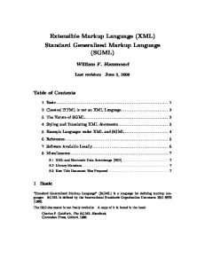
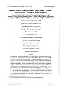
Figure 1.1: Time-course simulation of the repressilator model, imported from BioModels Database

and simulated in COPASI. The number of repressor proteins lacI, tetR and cI is shown. (taken from Waltemath et al. [2011a])

1.1

Motivation: A sample experiment The repressilator is a rather small, though famous, model that is capable of displaying rich and variable behaviors. We will use this model to demonstrate how a simulation experiment can be described simply and effectively. The simulation example is taken from Waltemath et al. [2011a]. The repressilator is a synthetic oscillating network of transcription regulators in Escherichia coli [Elowitz and Leibler, 2000]. The network is composed of the three repressor genes Lactose Operon Repressor (lacI), Tetracycline Repressor (tetR) and Repressor CI (cI), which code for proteins binding to the promoter of the other, blocking their transcription. The three inhibitions together in tandem, form a cyclic negative-feedback loop. To describe the interactions of the molecular species involved in the network, the authors built a simple mathematical model of coupled first-order differential equations. All six molecular species included in the network (three mRNAs, three repressor proteins) participated in creation (transcription/translation) and degradation processes. The model was used to determine the influence of the various parameters on the dynamic behavior of the system. In particular, parameter values were sought which induce stable oscillations in the concentrations of the system components. Oscillations in the levels of the three repressor proteins are obtained by numerical integration.

1.1.1

A simple time-course simulation The first experiment we intend to run on the model is the simulation that will lead to the oscillation shown in Figure 1c of the reference publication [Elowitz and Leibler, 2000]. This simulation experiment can be described as: 1. Import the model identified by the Unified Resource Identifier (URI) [Berners-Lee et al., 2005] urn:miriam:biomodels.db:BIOMD0000000012. 2. Select a deterministic method. 3. Run a uniform time course simulation for 1000 min with an output interval of 1 min. 4. Plot the amount of lacI, tetR and cI against time in a 2D Plot. Following those steps and performing the simulation in the simulation tool COPASI [Hoops et al., 2006] led to the result shown in Figure 1.1.

1.1.2

Applying pre-processing The fine-tuning of the model can be shown by adjusting parameters before simulation. When changing the initial values of the parameters protein copies per promoter and leakiness in protein copies per promoter the system’s behavior switches from sustained oscillation to asymptotic steady-state. The adjustments leading to that behavior may be described as: 1. Import the model as above.


5






and simulated in COPASI after modification of the initial values of the protein copies per promoter and the leakiness in protein copies per promoter. The number of repressor proteins lacI, tetR and cI is shown. (taken from Waltemath et al. [2011a])

2. Change the value of the parameter tps repr from “0.0005” to “1.3e-05”. 3. Change the value of the parameter tps active from “0.5 “ to “ 0.013“. 4. Select a deterministic method. 5. Run a uniform time course for the duration of 1000 min with an output interval of 1 min. 6. Plot the amount of lacI, tetR and cI against time in a 2D Plot. Figure 1.2 shows the result of the simulation.

1.1.3

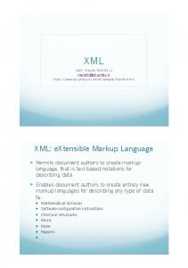
Applying post-processing The raw numerical output of the simulation steps may be subjected to data post-processing before plotting or reporting. In order to describe the production of a normalized plot of the time-course in the first example (section 1.1.1), depicting the influence of one variable on another (in phase-planes), one could define the following further steps: (Please note that the description steps 1 - 4 remain as given in section 1.1.1 above.) 5. Collect lacI(t) , tetR(t) and cI(t). 6. Compute the highest value for each of the repressor proteins, max(lacI(t)), max(tetR(t)), max(cI(t)). 7. Normalize the data for each of the repressor proteins by dividing each time point by the maximum value, i. e. lacI(t)/max(lacI(t) ), tetR(t)/max(tetR(t)) , and cI(t)/max(cI(t)). 8. Plot the normalized lacI protein as a function of the normalized cI, the normalized cI as a function of the normalized tetR protein, and the normalized tetR protein against the normalized lacI protein in a 2D plot. Figure 1.3 on the following page illustrates the result of the simulation after post-processing of the output data.


6






and simulated in COPASI, showing the normalized temporal evolution of repressor proteins lacI, tetR and cI in phase-plane. (taken from Waltemath et al. [2011a])


7






This document represents the technical specification of SED-ML. We also provide an XML Schema [W3C, 2004] and a UML class diagram representation of that XML Schema (Appendix A). UML class diagrams are a subset of the Unified Markup Language notation (UML, [OMG, 2009]). Sample experiment descriptions are given as XML snippets that comply with the XML Schema. It should however be noted that some of the concepts of SED-ML cannot be captured using XML Schema alone. In these cases it is this specification that is considered the normative document.


8



2. SED-ML technical specification


2.1


Conventions used in this document

2.1.1 UML Classes

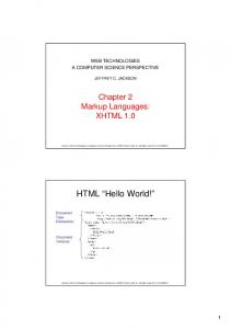
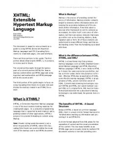
Figure 2.1: SED-ML UML class with class names and attributes

SED-ML class names always begin with upper case letters. If they are composed of different words, the camel case style is used, as in e. g. DataGenerator.

2.1.2

UML Relationships

2.1.2.1

UML Relation Types

Figure 2.2: UML Class connectors

Links between classes specify the connection of objects with each other (Figure 2.2). The different relation types used in the SED-ML specification include aggregation, composite aggregation, and generalisation. The label on the line is called symbol (label) and describes the relation of the objects of both classes. The association (Figure 2.3) indicates the existence of a connection between the objects of the participating classes. Often associations are directed to show how the label should be read (in which direction). Associations can be uni-directional (one arrowhead), or bidirectional (zero or two arrowheads).

Figure 2.3: UML Association

The aggregation (Figure 2.4 on the following page, top) indicates that the objects of the participating classes are connected in a way that one class (Whole) consists of several parts (Part). In an aggregation, the parts may be independent of the whole. For example, a car (Whole) has several parts called wheel (Part); however, the wheels can exist independently of the car while the car requires the wheels in order to function. The composite aggregation (Figure 2.4 on the next page, bottom) indicates that the objects of the participating classes are connected in a way that one class (Whole) consists of several parts (Part). In


9



A SED-ML UML class (Figure 2.1) consists of a class name (ClassName) and a number of attributes (attribute) each of a specific data type (type). The SED-ML UML specification does not make use of UML operations.


Figure 2.4: UML Aggregation (top) and Composition (bottom)

contrast to the aggregation, the subelements (Part) are dependent on the parent class (Whole). An example is that a university (Whole) consists of a number of departments (Part) which have a so-called “lifetime responsibility” with the university, e. g. if the university vanishes, the departments will vanish with it [Bell, 2003]. The generalisation (Figure 2.5) allows to extend classes (BaseClass) by additional properties. The derived class (DerivedClass) inherits all properties of the base class and defines additional ones. In the given example, an instance of DerivedClass has two attributes attribute1 and attribute2.

Figure 2.5: UML Generalisation

2.1.2.2 UML multiplicity

UML multiplicity defines the number of objects in one class that can be related to one object in the other class (also known as cardinality). Possible types of multiplicity include values (1), ranges (1..4), intervals (1,3,9), or combinations of ranges and intervals. The standard notation for “many” is the asterisk (*). Multiplicity can be defined for both sides of a relationship between classes. The default relationship is “many to many”. The example in Figure 2.6 expresses that a class is given by a professor, and a professor might give one to many classes.

Figure 2.6: UML Multiplicity in an Aggregation

2.1.3 XML Schema language elements The main building blocks of an XML Schema specification are:


10






• simple and complex types • element specifications XML Schema definitions create new types, declarations define new elements and attributes. The definition of new (simple and complex) types can be based on a number of already existing, predefined types (string, boolean, float). Simple types are restrictions or extensions of predefined types. Complex types describe how attribues can be assigned to elements and how elements can contain further elements. The current SED-ML XML Schema only makes use of complex type definitions. An example for a complex type definition is given in Listing 2.1: 1 2 3 4 5 6 7 8 9 10 11 12 13 14

Listing 2.1: Complex Type definition of the SED-ML computeChange element

It shows the declaration of an element called computeChange that is used in SED-ML to change mathematical expressions. The element is defined using an unnamed complex type which is built of further elements called listOfVariables, listOfParameters, and math. Additionally, the element computeChange has an attribute target declared. Please note that the definition of the elements inside the complex type are only referred to and will be found elsewhere in the schema. The nesting of elements in the schema can be expressed using the xs:sequence (a sequence of elements), xs:choice (an alternative of elements to choose from), or xs:all (a set of elements that can occur in any order) concepts. The current SED-ML XML Schema only uses the sequence of elements. 2.1.3.1

Multiplicities

The standard multiplicity for each defined element is 1. Explicit multiplicity is to be defined using the minOccurs and maxOccurs attributes inside the complex type definition, as shown in Listing 2.2. 1 2 3 4 5 6 7 8 9 10 11 12 13 14

Listing 2.2: Multiplicity for complex types in XML Schema

In this example, the dataGenerator type is build of a sequence of three elements: The listOfVariables element is not necessary for the definition of a valid dataGenerator XML structure (it may occur 0 times or once). The same is true for the listOfParameters element (it may as well occur 0 times or once). The math element, however, uses the implicit standard multiplicity – it must occur exactly 1 time in the dataGenerator specification.

2.1.4

Type extensions XML Schema offers mechanisms to restrict and extend previously defined complex types. Extensions add element or attribute declarations to existing types, while restrictions restrict the types by adding further characteristics and requirements (facets) to a type. An example for a type extension is given in Listing 2.3.


11



• attribute specifications

1 2 3 4 5 6 7 8 9 10 11 12 13 14 15 16 17 18 19


Listing 2.3: Definition of the sedML type through extension of SEDBase in SED-ML

The sedML element is an extension of the previously defined SEDBase type. It extends SEDBase by a sequence of five additional elements (listOfSimulations, listOfModels, listOfTasks, listOfDataGenerators, and listOfOutputs) and two new attributes version and level.


12





2.2


Concepts used in SED-ML

SED-ML files may encode pre-processing steps applied to the computational model, as well as post processing applied to the raw simulation data before output. The corresponding mathematical expressions are encoded using MathML 2.0 [Carlisle et al., 2001]. MathML is an international standard for encoding mathematical expressions using XML. It is also used as a representation of mathematical expressions in other formats, such as SBML and CellML, two of the languages supported by SED-ML. 2.2.1.1 MathML elements

In order to support for the SED-ML format easier to implement we restrict the MathML subset to the following elements: • token: cn, ci, csymbol, sep

• general : apply, piecewise, piece, otherwise, lambda • relational operators: eq, neq, gt, lt, geq, leq

• arithmetic operators: plus, minus, times, divide, power, root, abs, exp, ln, log, floor, ceiling, factorial • logical operators: and, or, xor, not

• qualifiers: degree, bvar, logbase

• trigonometric operators: sin, cos, tan, sec, csc, cot, sinh, cosh, tanh, sech, csch, coth, arcsin, arccos, arctan, arcsec, arccsc, arccot, arcsinh, arccosh, arctanh, arcsech, arccsch, arccoth • constants: true, false, notanumber, pi, infinity, exponentiale

• MathML annotations: semantics, annotation, annotation-xml 2.2.1.2 MathML Symbols

All the operations listed above only operate on scalar values. However, as one of SED-ML’s aims is to provide post processing on the results of simulation experiments, we need to enhance this basic set of operations by some aggregate functions. Therefore a defined set of MathML symbols that represent vector values are supported by SED-ML Level 1 Version 2. To simplify the use of SED-ML L1V2 the only symbols to be used are the identifiers of variables defined in the listOfVariables of DataGenerators. These variables represent the data collected from the simulation experiment with the associated task. 2.2.1.3 MathML functions

The following aggregate functions are available for use in SED-ML Level 1 Version 2. • min: Where the minimum of a variable represents the smallest value the simulation experiment yielded (Listing 2.4). 1 2 3 4 5 6

min variableId

Listing 2.4: Example for the use of the MathML min function.

• max : Where the maximum of a variables represents the largest value the simulation experiment yielded (Listing 2.5). 1 2 3 4 5 6

max variableId

Listing 2.5: Example for the use of the MathML max function.

• sum: All values of the variable returned by the simulation experiment are summed (Listing 2.6).


13



2.2.1 MathML subset


1 2 3 4 5 6


sum variableId

Listing 2.6: Example for the use of the MathML sum function.

1 2 3 4 5 6

product variableId

Listing 2.7: Example for the use of the MathML product function.

These represent the only exceptions. At this point SED-ML Level 1 Version 2 does not define a complete algebra of vector values. For more information see the description of the DataGenerator class.

2.2.2

URI Scheme URIs are needed at different points in SED-ML Level 1 Version 2. Firstly, they are the preferred mechanism to refer to model encodings. Secondly, they are used to specify the language of the referenced model. Thirdly, they enable addressing implicit model variables. Finally, annotations of SED-ML elements should be provided with a standardised annotation scheme. The use of a standardised URI Scheme ensures long-time availability of particular information that can unambiguously be identified.

2.2.2.1

Model references

The preferred way for referencing a model from a SED-ML file is adopted from the MIRIAM URI Scheme. MIRIAM enables identification of a data resource (in this case a model resource) by a predefined URN. A data entry inside that resource is identified by an ID. That way each single model in a particular model repository can be unambiguously referenced. To become part of MIRIAM resources, a model repository must ensure permanent and consistent model references, that is stable IDs. One model repository that is part of MIRIAM resources is the BioModels Database [Li et al., 2010]. Its data resource name in MIRIAM is urn:miriam:biomodels.db. To refer to a particular model, a standardised identifier scheme is defined in MIRIAM Resources1 . The ID entry maps to a particular model in the model repository. That model is never deleted. A sample BioModels Database ID is BIOMD0000000048. Together with the data resource name it becomes unambiguously identifiable by the URN urn:miriam:biomodels.db:BIOMD0000000048 (in this case referring to the 1999 Kholodenko model on EGFR signaling). SED-ML recommends to follow the above scheme for model references, if possible. SED-ML does not specify how to resolve the URNs. However, MIRIAM Resources offers web services to do so2 . For the above example of the urn:miriam:biomodels.db:BIOMD0000000048 model, the resolved URL may look like: • http://biomodels.caltech.edu/BIOMD0000000048 or • http://www.ebi.ac.uk/biomodels-main/BIOMD0000000048 depending on the physical location of the resource chosen to resolve the URN. An alternative means to obtain a model may be to provide a single resource containing necessary models and a SED-ML file. Although a specification of such a resource is beyond the scope of this document, one proposal – COMBINE archive format – is described in Appendix D. Further information on the source attribute referencing the model location is provided in Section 2.4.1.2. 1 http://www.ebi.ac.uk/miriam/ 2 http://www.ebi.ac.uk/miriam/


14



• product: All values of the variable returned by the simulation experiment are multiplied (Listing 2.7).



2.2.2.2 Language references

The list of URNs is available from http://sed-ml.org/. Further information on the language attribute is provided in Section 2.4.1.1. 2.2.2.3 Implicit variables

Some variables used in an experiment are not explicitly defined in the model, but may be implicitly contained in it. For example, to plot a variable’s behaviour over time, that variable is defined in an SBML model, while time is not explicitly defined. To overcome this issue and allow SED-ML to refer to such variables in a common way, the notion of implicit variables is used. Those variables are called symbols in SED-ML. They are defined following the idea of MIRIAM URNs and using the SED-ML URN scheme. The structure of the URNs is urn:sedml:symbol:implicit variable. To refer from a SED-ML file to the definition of time, for example, the URN is urn:sedml:symbol:time. The list of predefined symbols is available from the SED-ML site on http://sed-ml.org/. From that source, a mapping of SED-ML symbols on existing concepts in the languages supported by SED-ML is provided. 2.2.2.4 Annotations

When annotating SED-ML elements with semantic annotations, the MIRIAM URI Scheme should be used. In addition to providing the data type (e. g. PubMed) and the particular data entry inside that data type (e. g. 10415827), the relation of the annotation to the annotated element should be described using the standardised biomodels.net qualifier. The list of qualifiers, as well as further information about their usage, is available from http://www.biomodels.net/qualifiers/.

2.2.3

XPath usage XPath is a language for finding information in an XML document [Clarke and DeRose, 1999]. Within Level 1 Version 2, XPath version 1 expressions are used to identify nodes and attributes within an XML representation of a biological model in the following ways: 1. Within a Variable definition, where XPath identifies the model variable required for manipulation in SED-ML. 2. Within a Change definition, where XPath is used to identify the target XML to which a change should be applied. For proper application, XPath expressions should contain prefixes that allow their resolution to the correct XML namespace within an XML document. For example, the XPath expression referring to a species X in an SBML model: /sbml:sbml/sbml:model/sbml:listOfSpecies/sbml:species[@id=‘X’]

4 -CORRECT

is preferable to /sbml/model/listOfSpecies/species[@id=‘X’]

8 -INCORRECT

which will only be interpretable by standard XML software tools if the SBML file declares no namespaces (and hence is invalid SBML). Following the convention of other XPath host languages such as XPointer and XSLT, the prefixes used within XPath expressions must be declared using namespace declarations within the SED-ML document, and be in-scope for the relevant expression. Thus for the correct example above, there must also be an ancestor element of the node containing the XPath expression that has an attribute like:


15



To specify the language a model is encoded in, a set of pre-defined SED-ML URNs can be used. The structure of SED-ML language URNs is urn:sedml:language:name.version. SED-ML allows to specify a model representation format very generally as being XML, if no standardised representation format has been used to encode the model. On the other hand, one can be as specific as defining a model being in a particular version of a language, as “SBML Level 2, Version 2, Revision 1”.



xmlns:sbml=‘http://www.sbml.org/sbml/level3/version1/core’

(a different namespace URI may be used; the key point is that the prefix ‘sbml’ must match that used in the XPath expression).

KiSAO The Kinetic Simulation Algorithm Ontology (KiSAO, [Courtot et al., 2011]) is used in SED-ML to specify simulation algorithms and uniquely identify algorithm parameters. KiSAO is a community-driven approach of classifying and structuring simulation approaches by model characteristics and numerical characteristics. The ontology is available in OWL format from BioPortal at http://purl.bioontology. org/ontology/KiSAO. SED-ML refers to terms from KiSAO as referencing a simulation algorithm, or its parameters, solely through a name is error prone and ambiguous. After all, typing mistakes or language differences complicate the identification of the correct algorithm. Additionally, many algorithms exist under multiple names or abbreviation. The identification of a simulation algorithm through KISAO not only identifies the simulation algorithm to be used in the SED-ML simulation, it also enables software to find a related algorithm, if the specific implementation is not available. For example, software could decide to use the CVODE integration library for an analysis instead of a specific Runge Kutta 4,5 implementation. Should a particular simulation algorithm not exist within KISAO, please request one from the project homepage at http://www.biomodels.net/kisao/.

2.2.5

SED-ML resources Information on SED-ML can be found on http://sed-ml.org. The SED-ML XML Schema, the UML schema and related implementations, libraries, validators and so on can be found on the SED-ML sourceforge project page http://sed-ml.svn.sourceforge.net/.


16



2.2.4


2.3


General attributes and classes In this section we introduce attributes and concepts used repeatedly throughout the SED-ML specification.

Most objects in SED-ML carry an id attribute. The id attribute, if it exists for an object, is always required and identifies SED-ML constituents unambiguously. The data type for id is SId which is a datatype derived from the basic XML type string, but with restrictions about the characters permitted and the sequences in which those characters may appear. The definition is shown in Figure 2.7. letter digit idChar SId Figure 2.7:

::= ::= ::= ::=

’a’..’z’,’A’..’Z’ ’0’..’9’ letter | digit | ’ ’ ( letter | ’ ’ ) idChar*

The definition of the type SId

For a detailed description see also the SBML specification on the “Type SId” [Hucka et al., 2010, p. 11]. All ids have a global scope, i. e. the id must be unambiguous throughout a whole SED-ML document. As such it identifies the constituent it is related to. An example for a defined id is given in Listing 2.8. 1 2 3

[ MODEL DEFINITION ]

Listing 2.8: SED-ML identifier definition, e. g. for a model

The defined model carries the id m00001. If the model is referenced elsewhere in the SED-ML document, it is referred to by that id.

2.3.2 name Besides an id, a SED-ML constituent may carry an optional name. However, names do not have identifying character; several SED-ML constituents may carry the same name. The purpose of the name attribute is to keep a human-readable name of the constituent, e. g. for display to the user. In the XML Schema representation, names are of the data type String. Listing 2.9 extends the model definition in Listing 2.8 by a model name. 1 2 3

[ MODEL DEFINITION ]

Listing 2.9: SED-ML name definition, e. g. for a model

2.3.3 SEDBase SEDBase is the base class of SED-ML Level 1 Version 2. All other classes are derived from it. As such it provides means to attach additional information on all other classes (Figure 2.8 on the next page). That information can be specified by human readable Notes or custom Annotations.


17



2.3.1 id



Figure 2.8: The SEDBase class

Table 2.1 shows all attributes and sub-elements for the SEDBase element as defined by the SED-ML Level 1 Version 2 XML Schema. attribute metaido sub-elements noteso annotationo Table 2.1:

description page 18 description page 18 page 19

Attributes and nested elements for SEDBase. xyo denotes optional elements and at-

tributes.

2.3.3.1

metaid

The main purpose of the metaid attribute is to attach semantic annotations in form of the Annotation class to SED-ML elements. The type of metaid is XML ID and as such the metaid attribute is globally unique throughout the whole SED-ML document. An example showing how to link a semantic annotation to a SED-ML object via the metaid is given in the Annotation class description. 2.3.3.2

Notes

A note is considered a human-readable description of the element it is assigned to. It serves to display information to the user. Instances of the Notes class may contain any valid XHTML [Pemberton et al., 2002], ranging from short comments to whole HTML pages for display in a Web browser. The namespace URL for XHTML content inside the Notes class is http://www.w3.org/1999/xhtml. It may either be declared in the sedML XML element, or directly used in top level XHTML elements contained within the notes element. For further options of how to set the namespace and detailed examples, please refer to [Hucka et al., 2010, p. 14]. Table 2.2 shows all attributes and sub-elements for the Notes element as defined by the SED-ML Level 1 Version 2 XML Schema. Notes does not have any further sub-elements defined in SED-ML, nor attribute xmlns:string “http://www.w3.org/1999/xhtml” sub-elements well-formed content permitted in XHTML Table 2.2:

description page 21

Attributes and nested elements for Notes. xyo denotes optional elements and attributes.

attributes associated with it.


18



metaid



Listing 2.10 shows the use of the notes element in a SED-ML file as defined by the SED-ML Level 1 Version 2 XML Schema. 1 2 3 4 5 6

The enclosed simulation description shows the oscillating behaviour of the Repressilator model using deterministic and stochastic simulators .

In this example, the namespace declaration is inside the notes element and the note is related to the sedML root element of the SED-ML file. A note may, however, occur inside any SED-ML XML element, except note itself and annotation. 2.3.3.3

Annotation

An annotation is considered a computer-processible piece of information. Annotations may contain any valid XML content. For further guidelines on how to use annotations, we would like to encourage the reading of the corresponding section in the SBML specification [Hucka et al., 2010, pp. 14-16]. The style of annotations in SED-ML is briefly described in Section 2.2.2.4 on page 15. Table 2.3 shows all attributes and sub-elements for the Annotation element as defined by the SED-ML Level 1 Version 2 XML Schema. attribute none sub-elements none in the SED-ML namespace Table 2.3:

description description

Attributes and nested elements for Annotation. xyo denotes optional elements and at-

tributes.

Listing 2.11 shows the use of the annotation element in a SED-ML file as defined by the SED-ML Level 1 Version 2 XML Schema. 1 2 3 4 5 6 7 8 9 10 11 12 13 14 15 16 17 18 19

[..] [..]

Listing 2.11: The annotation element

In that example, a SED-ML model element is annotated with a reference to the original publication. The model contains an annotation that uses the biomodels.net model-qualifier isDescribedBy to link to the external resource urn:miriam:pubmed:10415827. In natural language the annotation content could be interpreted as “The model is described by the published article available from pubmed under ID 10643740 ”. The example annotation follows the proposed URI Scheme suggested by the MIRIAM reference standard. The MIRIAM URN can be resolved to the PubMED (http://pubmed.gov) publication with ID 10415827, namely the article “Alternating oscillations and chaos in a model of two coupled biochemical oscillators driving successive phases of the cell cycle.” published by Romond et al. in 1999.


19



Listing 2.10: The notes element



Each SED-ML Level 1 Version 2 document has a main class called SED-ML which defines the document’s structure and content (Figure 2.9). It consists of several parts; the parts are all connected to the SED-ML class through aggregation: the Model class (for model specification, see Section 2.4.1), the Simulation class (for simulation setup specification, see Section 2.4.3), the AbstractTask class (for the linkage of models and simulation setups, see Section 2.4.4), the DataGenerator class (for the definition of postprocessing, see Section 2.4.7), and the Output class (for the output specification, see Section 2.4.8). All of them are shown in Figure 2.9 and will be explained in more detail in the relevant sections of this document.

Figure 2.9: The sub-classes of SED-ML

Table 2.4 on the next page shows all attributes and sub-elements for the SED-ML element as defined by the SED-ML Level 1 Version 2 XML Schema. A SED-ML document needs to have the SED-ML namespace defined through the mandatory xmlns attribute. In addition, the SED-ML level and version attributes are mandatory. The basic XML structure of a SED-ML file is shown in listing 2.12 on the following page.


20



2.3.4 SED-ML top level element

attribute metaido xmlns level version sub-elements noteso annotationo listOfModelso listOfSimulationso listOfTaskso listOfDataGeneratorso listOfOutputso

http://journal.imbio.de description page 18 page 21 page 21 page 21 description page 18 page 19 page 28 page 29 page 30 page 30 page 31

Table 2.4: Attributes and nested elements for SED-ML. xyo denotes optional elements and attributes.

1 2 3 4 5 6 7 8 9 10 11 12 13 14

[ MODEL REFERENCES AND APPLIED CHANGES ] [ SIMULATION SETUPS ] [ MODELS LINKED TO SIMULATIONS ] [ DEFINITION OF POST - PROCESSING ] [ DEFINITION OF OUTPUT ]

Listing 2.12: The SED-ML root element

The root element of each SED-ML XML file is the sedML element, encoding version and level of the file, and setting the necessary namespaces. Nested inside the sedML element are the five lists serving as containers for the encoded data (listOfModels for all models, listOfSimulations for all simulations, listOfTasks for all tasks, listOfDataGenerators for all post-processing definitions, and listOfOutputs for all output definitions). 2.3.4.1

xmlns

The xmlns attribute declares the namespace for the SED-ML document. The pre-defined namespace for SED-ML documents is http://sed-ml.org/sed-ml/level1/version2. In addition, SED-ML makes use of the MathML namespace http://www.w3.org/1998/Math/MathML to enable the encoding of mathematical expressions in MathML 2.0. SED-ML uses a subset of MathML as described in Section 2.2.1 on page 13. SED-ML notes use the XHTML namespace http://www.w3.org/1999/xhtml. The Notes class is described in Section 2.3.3.2 on page 18. Additional external namespaces might be used in annotations. 2.3.4.2

level

The current SED-ML level is “level 1”. Major revisions containing substantial changes will lead to the definition of forthcoming levels. The level attribute is required and its value is a fixed decimal. For SED-ML Level 1 Version 2 the value is set to 1, as shown in the example in Listing 2.12. 2.3.4.3

version

The current SED-ML version is “version 2”. Minor revisions containing corrections and refinements of SED-ML elements, or new constructs which do not affect backwards compatibility, will lead to the definition of forthcoming versions. The version attribute is required and its value is a fixed decimal. For SED-ML Level 1 Version 2 the


21






value is set to 2, as shown in the example in Listing 2.12.

2.3.5

Reference relations The reference concept is used to refer to a particular element inside the SED-ML document. It may occur in six different ways in the SED-ML document:

2. as an association between a Variable and a Model (modelReference), 3. as an association between a Variable and an AbstractTask (taskReference), 4. as an association between a Task and the simulated Model (modelReference), 5. as an association between a Task and the Simulation run (simulationReference), or 6. as an association between an Output and a DataGenerator (dataReference). The definition of a Task object requires a reference to a particular Model object (modelReference, see Section 2.3.5.1 on page 22); furthermore, the Task object must be associated with a particular Simulation object (simulationReference, see Section 2.3.5.3 on page 23). Depending on the use of the reference relation in connection with a Variable object, it may take different roles: a. The reference association might occur between a Variable object and a Model object, e.g. if the variable is to define a Change. In that case the variable element contains a modelReference to refer to the particular model that contains the variable used to define the change (see Section 2.3.5.1 on page 22). b. If the reference is used as an association between a Variable object and an AbstractTask object inside the dataGenerator class, then the variable element contains a taskReference to unambiguously refer to an observable in a given task (see Section 2.3.5.2 on page 23). Four different types of data references exist in SED-ML Level 1 Version 2. They are used depending on the type of output for the simulation. A 2d plot has an xDataReference and a yDataReference assigned. A 3D plot has in addition a zDataReference assigned. To define a report, each data column has a dataReference assigned. 2.3.5.1 modelReference

The modelReference either represents a relation between two Model objects, a Variable object and a Model object, or a relation between a Task object and a Model object. The source attribute of a Model is allowed to reference either a URI or an SId to a second Model. Constructs where a model A refers to a model B and B to A (directly or indirectly) are invalid. If pre-processing needs to be applied to a model before simulation, then the model update can be specified by creating a Change object. In the particular case that a change must be calculated with a mathematical function, variables need to be defined. To refer to an existing entity in a defined Model, the modelReference is used. The modelReference attribute of the variable element contains the id of a model that is defined in the document. Listing 2.13 shows the use of the modelReference element in a SED-ML file as defined by the SED-ML Level 1 Version 2 XML Schema. 1 2 3 4 5 6 7 8 9

[..]


22



1. as an association between two Models (modelReference),


10 11 12 13 14 15


[ CALCULATION OF CHANGE ] [..]

Listing 2.13: SED-ML modelReference attribute inside a variable definition of a computeChange

In the example, a change is applied on model m0001. In the computeChange element a list of variables is defined. One of those variable is v1 which is defined in another model (cellML). The XPath expression given in the target attribute identifies the variable in the model which carries the ID cellML. The modelReference is also used to indicate that a Model object is used in a particular Task. Listing 2.14 shows how this can be done for a sample SED-ML document. 1 2 3 4

Listing 2.14: SED-ML modelReference definition inside a task element

The example defines two different tasks; the first one applies the simulation settings of simulation1 on model1, the second one applies the same simulation settings on model2. 2.3.5.2

taskReference

DataGenerator objects are created to apply post-processing to the simulation results before final output. For certain types of post-processing Variable objects need to be created. These link to a task defined within the listOfTasks from which the model that contains the variable of interest can be inferred. A taskReference association is used to realise that link from a Variable object inside a DataGenerator to an AbstractTask object. Listing 2.15 gives an example. 1 2 3 4 5 6 7 8

Listing 2.15: SED-ML taskReference definition inside a dataGenerator element

The example shows the definition of a variable v1 in a dataGenerator element. The variable appears in the model that is used in task t1. The task definition of t1 might look as shown in Listing 2.16. 1 2 3

Listing 2.16: Use of the reference relations in a task definition

Task t1 references the model model1. Therefore we can conclude that the variable v1 defined in Listing 2.15 targets an element of the model with ID model1. The targeting process itself will be explained in section 2.3.6.1 on page 25. 2.3.5.3 simulationReference

The simulationReference is used to refer to a particular Simulation in a Task. Listing 2.14 shows the reference to a defined simulation for a sample SED-ML document. In the example, both tasks t1 and t2 use the simulation settings defined in simulation1 to run the experiment. 2.3.5.4

dataReference

The dataReference is used to refer to a particular DataGenerator instance from an Output instance. Listing 2.17 shows the reference to a defined data set for a sample SED-ML document. 1 2 3


23



element


4 5 6


[..]

Listing 2.17: Example for the use of data references in a curve definition

2.3.6 Variable Variables are references to already existing entities, either existing in one of the defined models or implicitly defined symbols (Figure 2.10).

Figure 2.10: The Variable class

If the variable is defined through a reference to a model constituent, such as an SBML species, or to an entity within the SED-ML file itself, then the reference is specified using the target attribute. If the variable is defined through a reference to an implicit variable, rather than one explicitly appearing in the model, then the symbol attribute is used, which holds a SED-ML URI. A variable is always placed inside a listOfVariables. The symbol and target attributes must not be used together in a single instance of Variable, although at least one must be present. Table 2.5 shows all attributes and sub-elements for the Variable element as defined by the SED-ML Level 1 Version 2 XML Schema. attribute metaido id nameo target symbol taskReference modelReference sub-elements noteso annotationo Table 2.5:

description page 18 page 17 page 17 page 25 page 26 page 23 page 22 description page 18 page 19

Attributes and nested elements for Variable. xyo denotes optional elements and attributes.

A variable element must contain a taskReference if it occurs inside a listOfVariables inside a dataGenerator element. A variable element must contain a modelReference if it occurs inside a listOfVariables inside a computeChange element. A variable element appearing within a functionalRange or setValue element must contain a modelReference if and only if it references a model variable. Listing 2.18 shows the use of the variable element in a SED-ML file as defined by the SED-ML Level 1 Version 2 XML Schema. 1


24



In the example, the output type is a 2D plot, which defines one curve with id c1. A curve must refer to two different data generators which describe how to procure the data that is to be plotted on the x-axis and y-axis respectively.

2 3 4 5 6 7 8 9 10 11 12 13 14 15 16 17 18 19 20 21 22 23 24 25 26 27


[ FURTHER VARIABLE DEFINITIONS ] [..] [..] [..] [ FURTHER VARIABLE DEFINITIONS ] [..]

Listing 2.18: SED-ML variable definitions inside the computeChange element and inside the dataGenerator element

Listing 2.18 defines a variable v1 (line 7) to compute a change on a model constituent (referenced by the target attribute on computeChange in line 5). The value of v1 corresponds with the value of the targeted model constituent referenced by the target attribute in line 8. The second variable, v2 (line 21), is used inside a dataGenerator. As the variable is time as used in task1, the symbol attribute is used to refer to the SED-ML URI for time (line 21). 2.3.6.1

target

An instance of Variable can refer to a model constituent inside a particular model through an XPath expression stored in the target attribute. XPath can be used to unambiguously identify an element or attribute in an XML file. The target attribute may also be used to reference an entity within the SED-ML file itself, by containing a fragment identifier consisting of a hash character (#) followed by the id of the desired element. As of SED-ML Level 1 Version 2 this is only used to refer to ranges within a repeatedTask (see Listing 2.48 for an example). Listing 2.19 shows the use of the target attribute in a SED-ML file as defined by the SED-ML Level 1 Version 2 XML Schema. 1 2 3 4

Listing 2.19: SED-ML target definition

It should be noted that the identifier and names inside the SED-ML document do not have to match the identifiers and names that the model and its constituents carry in the model definition. In listing 2.19, the variable with ID v1 is defined. It is described as the TetR protein. The reference points to a species in the referenced SBML model. The particular species can be identified through its ID in the SBML model, namely PY. However, SED-ML also permits using identical identifiers and names as in the referenced models. The following Listing 2.20 is another valid example for the specification of a variable, but uses the same naming in the variable definition as in the original model (as opposed to Listing 2.19): 1 2 3 4

Listing 2.20: SED-ML variable definition using the original model identifier and name in SED-ML 1 2 3 4 5

The code of the model is changed in the way that its parameter with ID V mT is substituted by two other parameters V mT 1 and V mT 2. The target attribute defines that the parameter with ID V mT is to be changed. The newXML element then specifies the XML that is to be exchanged for that parameter. 2.4.2.4

RemoveXML

The RemoveXML class can be used to delete XML elements or attributes in the model that are addressed by the XPath expression (Figure 2.24).

Figure 2.24: The RemoveXML class

The XPath is specified in the required target attribute. Table 2.12 shows all attributes and sub-elements for the removeXml element as defined by the SED-ML Level 1 Version 2 XML Schema. attribute metaido id nameo target sub-elements noteso annotationo Table 2.12:

description page 18 page 17 page 17 page 25 description page 18 page 19

Attributes and nested elements for removeXML. xyo denotes optional elements and

attributes.

An example for the removal of an XML element from a model is given in Listing 2.38. 1 2 3 4


38



Listing 2.37: The changeXML element


5


Listing 2.38: The removeXML element

The code of the model is changed by deleting the reaction with ID V mT from the model’s list of reactions. ChangeAttribute

The ChangeAttribute class allows to define updates on the XML attribute values of the corresponding model (Figure 2.25).

Figure 2.25: The ChangeAttribute class

The ChangeXML class covers the possibilities provided by the ChangeAttribute class. That is, everything that can be expressed by a ChangeAttribute construct can also be expressed by a ChangeXML. However, for the common case of changing an attribute value ChangeAttribute is easier to use, and so it is recommended to use the ChangeAttribute for any changes of an XML attribute’s value, and to use the more general ChangeXML for other cases. ChangeAttribute requires to specify the target of the change, i. e. the location of the addressed XML attribute, and also the new value of that attribute. Note that the XPath expression in the target attribute must select a single attribute within the corresponding model. Table 2.13 shows all attributes and sub-elements for the changeAttribute element as defined by the SED-ML Level 1 Version 2 XML Schema. attribute metaido id nameo target newValue sub-elements noteso annotationo Table 2.13:

description page 18 page 17 page 17 page 25 page 39 description page 18 page 19

Attributes and nested elements for ChangeAttribute. xyo denotes optional elements and

attributes.

2.4.2.5.1

newValue

The mandatory newValue attribute assignes a new value to the targeted XML attribute. The example in Listing 2.39 shows the update of the initial concentration of two parameters inside an SBML model. 1 2 3 4 5 6


39



2.4.2.5


7


Listing 2.39: The changeAttribute element and its newValue attribute

2.4.2.6

ComputeChange

Figure 2.26: The ComputeChange class

The computed new value is described by a mathematical expression using a subset of MathML (see section 2.2.1 on page 13). The computation can use the value of variables from any model defined in the simulation experiment. Those variables need to be defined, and can then be addressed by their ID. A variable used in a ComputeChange must carry a modelReference attribute (page 22) but no taskReference attribute (page 23). To carry out the calculation it may be necessary to introduce additional parameters, that are not defined in any of the models used by the experiment. This is done through the parameter class, and such parameters are thereafter refered to by their ID. Finally, the change itself is specified using an instance of the Math class. Note that where a ComputeChange refers to another model, that model is not allowed to be modified by ComputeChanges which directly or indirectly refer to this model. In other words, cycles in the definitions of computed changes are prohibited, since then the new values would not be well defined. Table 2.14 on the next page shows all attributes and sub-elements for the computeChange element as defined by the SED-ML Level 1 Version 2 XML Schema. 2.4.2.6.1

Math

The Math element encodes mathematical functions. If used as an element of the ComputeChange class, it computes the change of the element or attribute addressed by the target attribute. Level 1 Version 2 supports the subset of MathML 2.0 shown in section 2.2.1. Listing 2.40 shows the use of the computeChange element in a SED-ML file as defined by the SED-ML Level 1 Version 2 XML Schema. 1 2 3 4 5


40



The ComputeChange class permits to change, prior to the experiment, the numerical value of any element or attribute of a model addressable by an XPath expression, based on a calculation (Figure 2.26).

attribute metaido id nameo target sub-elements noteso annotationo listOfVariableso listOfParameterso math Table 2.14:


description page 18 page 17 page 17 page 25 description page 18 page 19 page 27 page 28 page 40

Attributes and nested elements for computeChange. xyo denotes optional elements and

attributes.

6 7 8 9 10 11 12 13 14 15 16 17 18 19 20 21 22 23 24 25 26 27 28 29 30 31 32 33 34 35 36 37 38 39 40 41

S R n K n R n

Listing 2.40: The computeChange element

The example in Listing 2.40 computes a change of the variable sensor of the model model2. To do so, it uses the value of the variable regulator coming from model model1. In addition, the calculation used two additional parameters, the cooperativity n, and the sensitivity K. The mathematical expression in the mathML then computes the new initial value of sensor using the equation: S=S×

Rn K n +Rn

.

2.4.3 Simulation A simulation is the execution of some defined algorithm(s). Simulations are described differently depending on the type of simulation experiment to be performed (Figure 2.27 on the next page).


41






Simulation is an abstract class and serves as the container for the different types of simulation experiments. SED-ML Level 1 Version 2 offers the predefined simulation classes UniformTimeCourse, OneStep and SteadyState. Further simulation classes are planned for future versions of SED-ML, including simulation classes for bifurcation analysis. Simulation algorithms used for the execution of a simulation setup are defined in the Algorithm class. Table 2.15 shows all attributes and sub-elements for the simulation element as defined by the SED-ML Level 1 Version 2 XML Schema. attribute metaido id nameo sub-elements noteso annotationo algorithm Table 2.15:

description page 18 page 17 page 17 description page 18 page 19 page 42

Attributes and nested elements for simulation. xyo denotes optional elements and

attributes.

Listing 2.41 shows the use of the simulation element in a SED-ML file as defined by the SED-ML Level 1 Version 2 XML Schema. 1 2 3 4 5 6 7 8

[ SIMULATION SPECIFICATION ] [ SIMULATION SPECIFICATION ]

Listing 2.41: The SED-ML listOfSimulations element, defining two different simulations

Two timecourses with uniform range are defined. 2.4.3.1

Algorithm

SED-ML makes use of the KiSAO ontology (Section 2.2.4 on page 16) to refer to a term in the controlled vocabulary identifying the particular simulation algorithm to be used in the simulation. Each instance of the Simulation class must contain one reference to a simulation algorithm (Figure 2.28 on the following page).


42



Figure 2.27: The SED-ML Simulation class


Figure 2.28: The Algorithm class

Each instance of the Algorithm class must contain a KiSAO reference to a simulation algorithm. The reference should define the simulation algorithm to be used in the simulation as precisely as possible, and should be defined in the correct syntax, as defined by the regular expression KISAO:[0-9]{7}. The Algorithm class contains an optional list of parameters (algorithmParameter) that are used to parameterize the particular algorithm used in the simulation. Table 2.16 shows all attributes and sub-elements for the Algorithm element as defined by the SED-ML Level 1 Version 2 XML Schema. attribute metaido kisaoID sub-elements noteso annotationo algorithmParametero Table 2.16:

description page 18 page 16 description page 18 page 19 page 43

Attributes and nested elements for algorithm. xyo denotes optional elements and at-

tributes.

The example given in code snippet in Listing 2.41, completed by algorithm definitions results in the code given in Listing 2.42. 1 2 3 4 5 6 7 8

Listing 2.42: The SED-ML algorithm element for two different time course simulations, defining two different algorithms. KISAO:0000030 refers to the Euler forward method ; KISAO:0000021 refers to the StochSim nearest neighbor algorithm.

For both simulations, one algorithm is defined. In the first simulation s1 a deterministic approach has been chosen (Euler forward method), in the second simulation s2 a stochastic approach is used (Stochsim nearest neighbor). 2.4.3.2

AlgorithmParameter

The AlgorithmParameter class allows to parameterize a particular simulation algorithm. The set of possible parameters for a particular instance is determined by the algorithm that is referenced by the kisaoID of the enclosing algorithm element. Parameters of simulation algorithms are unambiguously referenced by the mandatory kisaoID attribute. Their value is set in the mandatory value attribute. 1 2 3 4 5

Listing 2.43:

The SED-ML algorithmParameter element setting the parameter value for the simulation algorithm. KISAO:0000032 refers to the explicit fourth-order Runge-Kutta method;


43






KISAO:00000211 refers to the absolute tolerance.

UniformTimeCourse

Figure 2.29: The UniformTimeCourse class

Table 2.17 shows all attributes and sub-elements for the uniformTimeCourse element as defined by the SED-ML Level 1 Version 2 XML Schema. attribute metaido id nameo initialTime outputStartTime outputEndTime numberOfPoints sub-elements noteso annotationo algorithm

description page 18 page 17 page 17 page 44 page 44 page 45 page 45 description page 18 page 19 page 42

Attributes and nested elements for uniformTimeCourse. xyo denotes optional elements and attributes.

Table 2.17:

Listing 2.44 shows the use of the uniformTimeCourse element in a SED-ML file as defined by the SED-ML Level 1 Version 2 XML Schema. 1 2 3 4 5 6

Listing 2.44: The SED-ML uniformTimeCourse element, defining a uniform time course simulation

over 2500 time units with 1000 simulation points. 2.4.3.3.1

initialTime

The attribute initialTime of type double represents the time from which to start the simulation. Usually this will be 0. Listing 2.44 shows an example. 2.4.3.3.2

outputStartTime

Sometimes a researcher is not interested in simulation results at the start of the simulation (i.e. the initial time). To accommodate this in SED-ML the uniformTimeCourse class uses the attribute outputStartTime of type double. To be valid the outputStartTime cannot be before initialTime. For an example, see Listing 2.44.


44



2.4.3.3

Journal of Integrative Bioinformatics, 12(2):262, 2015 2.4.3.3.3


outputEndTime

The attribute outputEndTime of type double marks the end time of the simulation. See Listing 2.44 for an example. numberOfPoints

When executed, the uniformTimeCourse simulation produces output on a regular grid starting with outputStartTime and ending with outputEndTime. The attribute numberOfPoints of type integer describes the number of points expected in the result. Software interpreting the uniformTimeCourse is expected to produce a first outputPoint at time outputStartTime and then numberOfPoints output points with the results of the simulation. Thus a total of numberOfPoints + 1 output points will be produced. Just because the output points lie on the regular grid described above, this does not mean that the simulation algorithm has to work with the same step size. Usually the step size the simulator chooses will be adaptive and much smaller than the required output step size. On the other hand a stochastic simulator might not have any new events occurring between two grid points. Nevertheless the simulator has to produce data on this regular grid. For an example, see Listing 2.44. 2.4.3.4

OneStep

Figure 2.30: The OneStep class

The SED-ML oneStep calculates one further output step for the model from its current state. Note that this does NOT necessarily equate to one integration step. The simulator is allowed to take as many steps as needed. However, after running oneStep, the desired output time is reached. Table 2.18 shows all attributes and sub-elements for the oneStep element as defined by the SED-ML Level 1 Version 2 XML Schema. attribute metaido id nameo step sub-elements noteso annotationo algorithm

description page 18 page 17 page 17 page 46 description page 18 page 19 page 42

Table 2.18: Attributes and nested elements for oneStep. xyo denotes optional elements and attributes.


45



2.4.3.3.4



Listing 2.45 shows the use of the oneStep element in a SED-ML file as defined by the SED-ML Level 1 Version 2 XML Schema. 1 2 3 4 5

Listing 2.45: The SED-ML oneStep element, specifying to apply the simulation algorithm for another

2.4.3.4.1

step

The oneStep class has one required attribute step of type double. It defines the next output point that should be reached by the algorithm, by specifying the increment from the current output point. Listing 2.45 shows an example. 2.4.3.5

SteadyState

The SteadyState class represents a steady state computation (as for example implemented by NLEQ or Kinsolve).

Figure 2.31: The SteadyState class

Table 2.19 shows all attributes and sub-elements for the steadyState element as defined by the SED-ML Level 1 Version 2 XML Schema.

Table 2.19:

attribute metaido id nameo

description page 18 page 17 page 17

sub-elements noteso annotationo algorithm


Attributes and nested elements for steadyState. xyo denotes optional elements and

attributes.

Listing 2.46 shows the use of the steadyState element in a SED-ML file as defined by the SED-ML Level 1 Version 2 XML Schema. 1 2 3 4


46



output step of size 0.1.


5


Listing 2.46: The SED-ML steadyState element, defining a steady state simulation with id steady.

2.4.4 Abstract Task

Figure 2.32: The SED-ML Abstract Task class

Table 2.20 shows all attributes and sub-elements for the abstractTask element as defined by the SED-ML Level 1 Version 2 XML Schema. attribute metaido id nameo sub-elements noteso annotationo Table 2.20:

description page 18 page 17 page 17 description page 18 page 19

Attributes and nested elements for abstractTask. xyo denotes optional elements and

attributes.

2.4.5 Task A task in SED-ML links a model to a certain simulation description via their respective identifiers (Figure 2.33 on the next page), using the modelReference and the simulationReference. The task class receives the id and name attributes from the AbstractTask.


47



An abstract task in SED-ML represents the base class for all SED-ML tasks. It is not meant to be instantiated directly.


Figure 2.33: The SED-ML Task class

In SED-ML Level 1 Version 2 it is only possible to link one simulation description to one model at a time. However, one can define as many tasks as needed within one experiment description. Please note that the tasks may be executed in any order, as determined by the implementation. Table 2.21 shows all attributes and sub-elements for the task element as defined by the SED-ML Level 1 Version 2 XML Schema. attribute metaido id nameo modelReference simulationReference sub-elements noteso annotationo Table 2.21:


Attributes and nested elements for task. xyo denotes optional elements and attributes.

Listing 2.47 shows the use of the task element in a SED-ML file as defined by the SED-ML Level 1 Version 2 XML Schema. 1 2 3 4 5 6

Listing 2.47: The task element

In the example, a simulation setting simulation1 is applied first to model1 and then is applied to model2.

2.4.6 Repeated Task The repeatedTask class provides a generic looping construct, allowing complex tasks to be represented by composing separate steps. It performs a specified task (or sequence of tasks) multiple times (where the exact number is specified through a range construct), while allowing specific quantities in the model to be altered at each iteration (as defined in the listOfChanges).


48






The RepeatedTask inherits from AbstractTask. Additionally it has two required attributes range and resetModel as well as child elements listOfRanges, listOfChanges and listOfSubTasks. Of these only listOfChanges is optional.

Figure 2.34: The SED-ML RepeatedTask class

Table 2.22 shows all attributes and sub-elements for the repeatedTask element as defined by the SED-ML Level 1 Version 2 XML Schema. attribute metaido id nameo range resetModel sub-elements noteso annotationo range changeo subTasko Table 2.22:

description page 18 page 17 page 17 page 50 page 50 description page 18 page 19 page 50 page 53 page 53

Attributes and nested elements for repeatedTask. xyo denotes optional elements and

attributes.

Listing 2.48 shows the use of the repeatedTask element in a SED-ML file as defined by the SED-ML Level 1 Version 2 XML Schema. 1

2 3 4


49



Note that the order of activities within each iteration of a repeatedTask is as follows. Firstly the model is reset, if specified by the resetModel attribute. Secondly any changes to the model specified by setValue elements are made. Finally, the subTasks are executed once each in order.

5 6 7 8 9 10 11 12 13 14 15 16 17 18 19 20 21 22 23 24 25


1 4 10 val

Listing 2.48: The repeatedTask element

In the example, task1 is repeated three times, each time with a different value for a model parameter w. 2.4.6.1

The range attribute

The repeatedTask class has a required attribute range of type SId. It specifies which range defined in the listOfRanges this repeated task iterates over. Listing 2.48 shows an example of a repeatedTask iterating over a single range comprising the values: 1, 4 and 10. If there are multiple ranges in the listOfRanges, then only the master range identified by this attribute determines how many iterations there will be in the repeatedTask. All other ranges must allow for at least as many iterations as the master range, and will be moved through in lock-step; their values can be used in setValue constructs. 2.4.6.2

The resetModel attribute

The repeatedTask class has a required attribute resetModel of type boolean. It specifies whether the model should be reset to the initial state before processing an iteration of the defined subTasks. Here initial state refers to the state of the model as given in the listOfModels. In the example in Listing 2.48 the repeated task is not to be reset, so a change is made, task1 is carried out, another change is made, then task1 continues from there, another change is applied, and task1 is carried out a last time. 2.4.6.3 The listOfRanges

Ranges represent the iterative element of the nested simulation experiment that provides the collection of values to iterate over. In order to be able to refer to the current value of a range element, an id attribute is added. When the value of the id attribute is used in a listOfVariables within the repeated task class its value is to be replaced with the current value of the range. There are three different range types permitted in the listOfRanges: UniformRange, VectorRange and FunctionalRange. They each inherit from an abstract Range class. 2.4.6.3.1

Range

The Range class is abstract and exists solely as the base class for the different types of range. Therefore, a SED-ML document will only contain the derived classes listed below.


50




Journal of Integrative Bioinformatics, 12(2):262, 2015 UniformRange

Figure 2.35: The SED-ML UniformRange class

The UniformRange is quite similar to what is used in the UniformTimeCourse simulation class. This range is defined through four mandatory attributes: start, the start value; end, the end value and numberOfPoints that contains the number of points the range contains. A fourth attribute type that can take the values linear or log determines whether to draw the values logarithmically (with a base of 10) or linearly. For example: 1

Listing 2.49: The UniformRange element

As for UniformTimeCourse, this range will actually produce 101 values uniformly spaced on the interval [0, 10], in ascending order. The following logarithmic example generates the three values 1, 10 and 100. 1

Listing 2.50: The UniformRange element with a logarithmic range.

2.4.6.3.3

VectorRange

Figure 2.36: The SED-ML VectorRangeClass class

A VectorRange describes an ordered collection of real values, listing them explicitly within child value elements. For example, the range below iterates over the values 1, 4 and 10 in that order.


51



2.4.6.3.2



1 2 3 4 5


1 4 10

Listing 2.51: The VectorRange element

FunctionalRange

Figure 2.37: The SED-ML FunctionalRange class

A FunctionalRange constructs a range through calculations that determine the next value based on the value(s) of other range(s) or model variables. In this it is quite similar to the ComputeChange element, and shares some of the same child elements. It consists of an optional attribute range, two optional elements listOfVariables and listOfParameters, and a required element math. The optional attribute range may be used as a shorthand to specify the id of another Range. The current value of the referenced range may then be used within the function defining this FunctionalRange, just as if that range had been referenced using a variable element, except that the id of the range is used directly. In other words, whenever the expression contains a ci element that contains the value specified in the range attribute, the value of the referenced range is to be inserted. In the listOfVariables, variable elements define identifiers refering to model variables or range values, which may then be used within the math expression. These references always retrieve the current value of the model variable or range at the current iteration of the enclosing repeatedTask. For a model not being simulated by any subTask, the initial state of the model is used. The function encompasses the mathematical expression that is used to compute the value for the functional range at each iteration of the enclosing repeatedTask. For example: 1 2 3 4 5 6 7 8 9 10 11 12 13

w index


52



2.4.6.3.4


14


Listing 2.52: An example of a functionalRange where a parameter w of model model2 is multiplied

by index each time it is called.

1 2 3 4 5 6 7 8 9 10 11 12 13 14 15 16 17 18 19 20 21 22 23 24 25 26 27 28 29 30 31 32 33 34

8 index 1 0.1 index 4 index 6 8

Listing 2.53: A functionalRange element that returns 8 if index is smaller than 1, 0.1 if index is between 4 and 6, and 8 otherwise.

2.4.6.4

The listOfChanges

The listOfChanges element, when present, contains one or more setValue elements. These elements allow the modification of values in the model prior to the next execution of the subTasks. A setValue element inherits from the computeChange class, which allows it to compute arbitrary expressions involving a number of variables and parameters. The element setValue adds a mandatory modelReference attribute, and two optional attributes range and symbol. The value to be changed is identified via the combination of the attributes modelReference and either symbol or target, in order to select an implicit or explicit variable within the referenced model. As in functionalRange, the atribute range may be used as a shorthand for refering to the range whose values will be used to compute a value for the specified model element. The child math contains the expression computing the value by refering to optional parameters, variables or ranges. Again as for functionalRange, variable references always retrieve the current value of the model variable or range at the current iteration of the enclosing repeatedTask. For a model not being simulated by any subTask, the initial state of the model is used. 1 2 3 4 5 6 7 8

current

Listing 2.54: A setValue element setting w to the values of the range with id current.

2.4.6.5

The listOfSubTasks

The listOfSubTasks contains one or more subTask elements that specify what simulations are to be performed by the RepeatedTask. All subTasks have to be carried out sequentially, each continuing from


53



Here is another example, this time using the values in a piecewise expression:



1 2 3 4

Listing 2.55: The subTask element. In this example the task task2 has to be carried out before task1.

2.4.7 DataGenerator The DataGenerator class prepares the raw simulation results for later output (Figure 2.38). It encodes the post-processing to be applied to the simulation data. The post-processing steps could be anything, from simple normalisations of data to mathematical calculations.

Figure 2.38: The SED-ML DataGenerator class

Each instance of the DataGenerator class is identifiable within the experiment by its unambiguous id. It can be further characterised by an optional name. The related Math class contains a mathML expression for the calculation of the data generator. Mathematical functions available for the specification of data generators are given in Section 2.2.1 on page 13. Variable and Parameter instances can be used to encode the mathematical expression. Table 2.23 shows all attributes and sub-elements for the dataGenerator element as defined by the SEDML Level 1 Version 2 XML Schema.

Table 2.23:

attribute metaido id nameo


sub-elements math noteso annotationo variableo parametero

description page 40 page 18 page 19 page 24 page 26

Attributes and nested elements for dataGenerator. xyo denotes optional elements and

attributes.

Listing 2.56 shows the use of the dataGenerator element in a SED-ML file as defined by the SED-ML Level 1 Version 2 XML Schema. 1 2 3 4 5


54



the current model state (i.e. as at the end of the previous subTask, assuming it simulates the same model), and with their results concatenated (thus appearing identical to a single complex simulation). The subTask itself has one required attribute task that references the id of another task defined in the listOfTasks. The order in which to run multiple subTasks should be specified using order attributes on the subTask elements; if these are omitted the ordering is given by the order of the subTask elements. In order to establish that one subTask should be carried out before another its order attribute has to have a lower number (c.f. Listing 2.55).

6 7 8 9 10 11 12 13 14 15 16 17 18 19 20 21


time v1

Listing 2.56: Definition of two dataGenerator elements, time and LaCI repressor

The listOfDataGenerator contains two dataGenerator elements. The first one, d1, refers to the task definition t1 (which itself refers to a particular model), and from the corresponding model it reuses the symbol time. The second one, d2, references a particular species defined in the same model (and referred to via the taskReference="t1"). The model species with ID PX is reused for the data generator d2 without further post-processing.

2.4.8 Output The Ouput class describes how the results of a simulation should be presented to the user (Figure 2.39).

Figure 2.39: The SED-ML Output class

It does not contain the data itself, but the type of output and the data generators used to produce a particular output. The types of output pre-defined in SED-ML Level 1 Version 2 are plots and reports. The output can be defined as a 2D plot or alternatively as a 3D plot. Note that even though the terms “2D plot” and “3D plot” are used, the exact type of plot is not specified. In other words, whether the 3D plot represents a surface plot, or three dimensional lines in space, cannot be distinguished by SED-ML alone. It is expected that applications use annotations for this purpose. Table 2.24 on the following page shows all attributes and sub-elements for the output element as defined by the SED-ML Level 1 Version 2 XML Schema. 2.4.8.1

Plot2D

A 2 dimensional plot (Figure 2.40 on the next page) contains a number of curve definitions.


55




attribute metaido id nameo sub-elements noteso annotationo plot2Do plot3Do reporto Table 2.24:


description page 18 page 17 page 17 description page 18 page 19 page 55 page 57 page 57

Attributes and nested elements for output. xyo denotes optional elements and attributes.

Figure 2.40: The SED-ML Plot2D class

Table 2.25 shows all attributes and sub-elements for the plot2D element as defined by the SED-ML Level 1 Version 2 XML Schema. attribute metaido id nameo sub-elements noteso annotationo curve Table 2.25:


Attributes and nested elements for plot2D. xyo denotes optional elements and attributes.

Listing 2.57 shows the use of the listOfCurves element in a SED-ML file as defined by the SED-ML Level 1 Version 2 XML Schema. 1 2 3 4 5 6 7 8

[ CURVE DEFINITION ] [ FURTHER CURVE DEFINITIONS ]

Listing 2.57: The plot2D element with the nested listOfCurves element

The listing shows the definition of a 2 dimensional plot containing one curve element inside the listOfCurves. The curve definition follows in Section 2.4.9.1 on page 58.


56




Journal of Integrative Bioinformatics, 12(2):262, 2015 2.4.8.2


Plot3D

Figure 2.41: The SED-ML Plot3D class

Table 2.26 shows all attributes and sub-elements for the plot3D element as defined by the SED-ML Level 1 Version 2 XML Schema. attribute metaido id nameo sub-elements noteso annotationo surface Table 2.26:


Attributes and nested elements for plot3D. xyo denotes optional elements and attributes.

Listing 2.58 shows the use of the plot3D element in a SED-ML file as defined by the SED-ML Level 1 Version 2 XML Schema. 1 2 3 4 5 6 7 8

[ SURFACE DEFINITION ] [ FURTHER SURFACE DEFINITIONS ]

Listing 2.58: The plot3D element with the nested listOfSurfaces element

The example defines a surface for the 3 dimensional plot. The surface definition follows in Section 2.4.9.2 on page 60. 2.4.8.3 The Report class

The Report class defines a data table consisting of several single instances of the DataSet class (Figure 2.42 on the next page). Its output returns the simulation result in actual numbers. The particular columns of the report table are defined by creating an instance of the DataSet class for each column.


57



A 3 dimensional plot (Figure 2.41) contains a number of surface definitions.



Table 2.27 shows all attributes and sub-elements for the report element as defined by the SED-ML Level 1 Version 2 XML Schema. attribute metaido id nameo sub-elements noteso annotationo dataSet Table 2.27:


Attributes and nested elements for report. xyo denotes optional elements and attributes.

Listing 2.59 shows the use of the listOfDataSets element in a SED-ML file as defined by the SED-ML Level 1 Version 2 XML Schema. 1 2 3 4 5 6 7

[DATA REFERENCE ]

Listing 2.59: The report element with the nested listOfDataSets element

The simulation result itself, i. e. concrete result numbers, are not stored in SED-ML, but the directive how to calculate them from the output of the simulator is provided through the dataGenerator. The encoding of simulation results is outside the scope of SED-ML, but other efforts exist, for example the Systems Biology Result Markup Language (SBRML, [Dada et al., 2010]).

2.4.9

Output components

2.4.9.1

Curve

One or more instances of the Curve class define a 2D plot. A curve needs a data generator reference to refer to the data that will be plotted on the x-axis, using the xDataReference. A second data generator reference is needed to refer to the data that will be plotted on the y-axis, using the yDataReference.

Figure 2.43: The SED-ML Curve class

Table 2.28 on the following page shows all attributes and sub-elements for the curve element as defined


58



Figure 2.42: The SED-ML Report class



attribute metaido id nameo logX xDataReference logY yDataReference sub-elements noteso annotationo Table 2.28:

description page 18 page 17 page 17 page 59 page 59 page 59 page 59 description page 18 page 19

Attributes and nested elements for curve. xyo denotes optional elements and attributes.

Listing 2.60 shows the use of the curve element in a SED-ML file as defined by the SED-ML Level 1 Version 2 XML Schema. 1 2 3

Listing 2.60: The SED-ML curve element, defining the output curve showing the result of simulation

for the referenced dataGenerators

Here, only one curve is created, results shown on the x-axis are generated by the data generator dg1, results shown on the y-axis are generated by the data generator dg2. Both dg1 and dg2 need to be already defined in the listOfDataGenerators. The x-axis is plotted logarithmically. 2.4.9.1.1

logX

logX is a required attribute of the Curve class and defines whether or not the data output on the x-axis is logarithmic. The data type of logX is boolean. To make the output on the x-axis of a plot logarithmic, logX must be set to “true”, as shown in the sample Listing 2.60. logX is also used in the definition of a Surface output. 2.4.9.1.2

logY

logY is a required attribute of the Curve class and defines whether or not the data output on the y-axis is logarithmic. The data type of logY is boolean. To make the output on the y-axis of a plot logarithmic, logY must be set to “true”, as shown in the sample Listing 2.60. logY is also used in the definition of a Surface output. 2.4.9.1.3

xDataReference

The xDataReference is a mandatory attribute of the Curve object. Its content refers to a dataGenerator ID which denotes the DataGenerator object that is used to generate the output on the x-axis of a Curve in a 2D Plot. The xDataReference data type is string. However, the valid values for the xDataReference are restricted to the IDs of already defined DataGenerator objects. An example for the definition of a curve is given in Listing 2.60. xDataReference is also used in the definition of the x-axis of a Surface in a 3D Plot. 2.4.9.1.4

yDataReference

The yDataReference is a mandatory attribute of the Curve object. Its content refers to a dataGenerator ID which denotes the DataGenerator object that is used to generate the output on the y-axis of a Curve in a 2D Plot. The yDataReference data type is string. However, the number of valid values for the yDataReference is restricted to the IDs of already defined DataGenerator objects. An example for the definition of a curve is given in Listing 2.60. yDataReference is also used in the


59



by the SED-ML Level 1 Version 2 XML Schema.



definition of the y-axis of a Surface in a 3D Plot. Surface

A surface is a three-dimensional figure representing a simulation result (Figure 2.44).

Figure 2.44: The SED-ML Surface class

Creating an instance of the Surface class requires the definition of three different axes, that is which data to plot on which axis and in which way. The aforementioned xDataReference and yDataReference attributes define the according data generators for both the x- and y-axis of a surface. In addition, the zDataReference attribute defines the output for the z-axis. All axes might be logarithmic or not. This can be specified through the logX, logY, and the logZ attributes in the according dataReference elements. Table 2.29 shows all attributes and sub-elements for the surface element as defined by the SED-ML Level 1 Version 2 XML Schema. Listing 2.61 shows the use of the surface element in a SED-ML file attribute metaido id nameo logX xDataReference logY yDataReference logZ zDataReference sub-elements noteso annotationo Table 2.29:

description page 18 page 17 page 17 page 59 page 59 page 59 page 59 page 61 page 61 description page 18 page 19

Attributes and nested elements for surface. xyo denotes optional elements and attributes.

as defined by the SED-ML Level 1 Version 2 XML Schema. 1 2 3 4 5

[ FURTHER SURFACE DEFINITIONS ]

Listing 2.61: The SED-ML surface element, defining the output showing the result of the referenced

task

Here, only one surface is created, results shown on the x-axis are generated by the data generator dg1, results shown on the y-axis are generated by the data generator dg2, and results shown on the z-axis are generated by the data generator dg3. All dg1, dg2 and dg3 need to be already defined in the


60



2.4.9.2



listOfDataGenerators. 2.4.9.2.1

logZ

logZ is a required attribute of the Surface class and defines whether or not the data output on the z-axis is logarithmic. The data type of logZ is boolean. To make the output on the z-axis of a surface plot logarithmic, logZ must be set to “true”, as shown in the sample Listing 2.61. zDataReference

The zDataReference is a mandatory attribute of the Surface object. Its content refers to a dataGenerator ID which denotes the DataGenerator object that is used to generate the output on the z-axis of a 3D Plot. The zDataReference data type is string. However, the valid values for the zDataReference are restricted to the IDs of already defined DataGenerator objects. An example using the zDataReference is given in Listing 2.61 on page 60. 2.4.9.3

DataSet

The DataSet class holds definitions of data to be used in the Report class (Figure 2.45).

Figure 2.45: The SED-ML DataSet class

Data sets are labeled references to instances of the DataGenerator class. Table 2.30 shows all attributes and sub-elements for the dataSet element as defined by the SED-ML Level 1 Version 2 XML Schema. attribute metaido id nameo dataReference label sub-elements noteso annotationo


Table 2.30: Attributes and nested elements for dataSet. xyo denotes optional elements and attributes.

2.4.9.3.1

label

Each data set in a Report does have to carry an unambiguous label. A label is a human readable descriptor of a data set for use in a report. For example, for a tabular data set of time series results, the label could be the column heading. 2.4.9.3.2

dataReference

The dataReference attribute contains the ID of a dataGenerator element and as such represents a link to it. The data produced by that particular data generator fills the according data set in the report. Listing 2.62 on the next page shows the use of the dataSet element in a SED-ML file as defined by the SED-ML Level 1 Version 2 XML Schema.


61



2.4.9.2.2


1 2 3


Listing 2.62: The SED-ML dataSet element, defining a data set containing the result of the referenced


task


62




The SED-ML specification has been developed with the input of many people. The following individuals served as past SED-ML Editors and contributed to SED-ML specifications. Their efforts helped shape what SED-ML is today. • Richard Adams • Andrew Miller Moreover, we would like to thank all the participants of the meetings where SED-ML has been discussed as well as the members of the SED-ML community.


63



3. Acknowledgements



Figure A.1 shows the complete UML diagram of the SED-ML. It gives the full picture of all implemented classes (see the XML Schema definition on page 65).

Figure A.1: The SED-ML UML class diagram


64



A. SED-ML UML Overview



Listing B.1 shows the full SED-ML XML Schema. The code is commented inline. 1 2 3 4

5 6 7 8 9 10 11 12 13 14 15 16 17

The type SId is used throughout SED -ML as the type of the ’id ’ attributes on SED -ML elements .

18 19 20 21 22 23

24 25 26 27 28 29 30 31 32 33 34 35 36 37 38 39 40 41 42 43 44 45 46 47 48 49 50 51 52 53 54 55 56 57 58 59 60 61 62 63 64 65 66 67 68

The SEDBase type is the base type of all main types in SED -ML. It serves as a container for the annotation of any part of the experiment description .


65



B. XML Schema

69 70 71 72 73 74 75 76 77 78 79 80 81 82 83 84 85 86


87 88 89 90 91 92 93 94 95

96 97 98 99 100 101 102 103 104 105 106 107 108 109 110 111 112 113 114

115 116 117 118 119 120 121 122 123 124 125 126 127 128 129 130 131

132 133 134 135 136 137 138 139 140 141 142 143 144 145 146 147 148 149 150 151 152 153 154 155 156 157


66




158 159 160 161 162 163 164 165 166 167 168 169 170 171 172 173 174 175 176 177 178 179 180 181 182 183 184 185 186 187 188 189 190 191 192 193 194 195 196


197 198 199 200 201 202 203 204 205 206 207 208 209 210 211 212 213 214 215 216 217 218 219 220 221 222 223 224 225 226 227 228 229 230 231 232 233 234 235 236 237 238 239 240 241 242 243 244 245 246


67




247 248 249 250 251 252 253 254 255 256 257 258 259 260 261


262 263 264 265 266 267 268 269 270 271 272 273 274 275 276 277 278 279 280 281 282 283 284 285 286 287 288 289 290 291 292 293 294 295 296 297 298 299 300 301 302 303 304 305 306 307 308 309 310 311 312 313 314 315 316 317 318 319 320 321 322 323 324 325 326 327 328 329 330 331 332 333 334 335


68




336 337 338 339 340 341 342 343 344 345 346 347 348 349 350 351 352 353 354 355 356 357 358 359 360 361 362 363 364 365 366 367 368


369 370 371 372 373 374 375 376 377 378 379 380 381 382 383 384

385 386 387 388 389 390 391 392 393 394 395 396 397 398 399 400 401 402 403 404 405 406 407 408 409 410 411 412 413 414 415 416 417 418 419 420 421 422 423 424


69





425 426 427 428 429


431 432 433 434 435 436 437 438 439 440 441 442 443 444 445 446 447 448 449 450 451 452 453 454 455 456 457 458 459 460 461 462

463 464 465 466 467 468 469 470 471 472 473 474 475 476 477 478 479 480 481 482 483 484 485 486 487 488 489 490 491 492 493 494 495 496 497 498 499 500 501 502 503 504 505 506 507 508 509 510 511 512 513


70



430

514 515 516 517 518 519 520 521 522 523 524 525 526 527 528 529 530 531 532 533 534 535 536 537 538 539 540 541 542 543 544 545 546 547 548 549 550 551 552 553 554 555 556 557 558 559 560 561 562 563 564 565 566 567 568 569 570 571 572 573 574 575 576 577 578 579 580 581 582 583 584 585 586 587 588 589 590 591 592 593 594 595 596 597 598 599 600 601 602



71




603 604 605 606 607 608 609 610 611 612 613 614 615 616 617 618 619 620 621 622 623 624 625 626 627 628 629 630 631 632 633 634 635 636 637 638 639


Listing B.1: The SED-ML XML Schema definition


72






This appendix present a few examples SED-ML uses. These examples are only illustrative and do not intend to demonstrate the full capabilities of SED-ML. Please read the specification for a for a more comprehensive view (Chapter 2). The current examples make use of models encoded in SBML and CellML. It is important to remember that SED-ML is not restricted to those formats, but can be used with models encoded in many formats, so long as they are serialized in XML. A list of formats known to have been used, at least tentatively, with SED-ML is available on http://sed-ml.org/.


73



C. Examples


Le Loup Model (SBML) The following example provides a SED-ML description for the simulation of the model based on the publication by Leoup, Gonze and Goldbeter “Limit Cycle Models for Circadian Rhythms Based on Transcriptional Regulation in Drosophila and Neurospora” (PubMed ID: 10643740). This model is referenced by its SED-ML ID model1 and refers to the model with the MIRIAM URN urn: miriam:biomodels.db:BIOMD0000000021. Software applications interpreting this example know how to dereference this URN and access the model in BioModels Database [Le Novère et al., 2006]. A second model is defined in l. 11 of the example, using model1 as a source and applying even further changes to it, in this case updating two model parameters. One simulation setup is defined in the listOfSimulations. It is a uniformTimeCourse over 380 time units, providing 1000 output points. The algorithm used is the CVODE solver, as denoted by the KiSAO ID KiSAO:0000019. A number of dataGenerators are defined in ll. 23-62. Those are the prerequisite for defining the outputs of the simulation. The first dataGenerator named time collects the simulation time. tim1 in l. 31 maps on the Mt entity in the model that is used in task1 which here is the model with ID model1. The dataGenerator named per-tim1 in l. 39 maps on the Cn entity in model1. Finally the fourth and fifth dataGenerators map on the Mt and per-tim entity respectively in the updated model with ID model2. The output defined in the experiment consists of three 2D plots. The first plot has two different curves (ll. 65-70) and provides the time course of the simulation using the tim mRNA concentrations from both simulation experiments. The second plot shows the per-tim concentration against the tim concentration for the oscillating model. And the third plot shows the same plot for the chaotic model. The resulting three plots are shown in Figure C.1.

tim mRNA with Oscillation and Chaos tim mRNA

9

tim mRNA limit cycle (Oscillation)

tim mRNA (changed parameters)

tim mRNA

4.0

8

3.5

7

3.0

6

2.5

5

2.0

4 1.5

3

1.0

2

0.5

1 0

0.0 0

50

100

150

200

250

300

350

400

0.0

0.5

1.0

1.5

2.0

2.5

3.0

3.5

tim mRNA limit cycle (chaos) tim mRNA (changed parameters)

9 8 7 6 5 4 3 2 1 0 0

1

2

3

4

5

Figure C.1: The simulation result gained from the simulation description given in Listing C.1

1 2 3 4 5


74



C.1


6 7 8 9 10 11 12 13 14 15 16 17 18 19 20 21 22 23 24 25 26 27 28 29 30 31 32 33 34 35 36 37 38 39 40 41 42 43 44 45 46 47 48 49 50 51 52 53 54 55 56 57 58 59 60 61 62 63 64 65 66 67 68 69 70 71 72 73 74 75 76 77 78 79 80 81 82 83 84


t v1 v1a v2 v2a

Listing C.1: LeLoup Model Simulation Description in SED-ML


75





Le Loup Model (CellML) The following example provides a SED-ML description for the simulation of the model based on the publication by Leloup, Gonze and Goldbeter “Limit Cycle Models for Circadian Rhythms Based on Transcriptional Regulation in Drosophila and Neurospora” (PubMed ID: 10643740). Whereas the previous example used SBML to encode the simulation experiment, here the model is taken from the CellML Model Repository [Lloyd et al., 2008]. The original model used in the simulation experiment is referred to using a URL (http://models.cellml. org/workspace/leloup_gonze_goldbeter_1999/@@rawfile/7606a47e222bc3b3d9117baa08d2e7246d67eedd/ leloup_gonze_goldbeter_1999_a.cellml, ll. 14). A second model is defined in l. 15 of the example, using model1 as a source and applying even further changes to it, in this case updating two model parameters. One simulation setup is defined in the listOfSimulations. It is a uniformTimeCourse over 380 time units, using 1000 simulation points. The algorithm used is the CVODE solver, as denoted by the KiSAO ID KiSAO:0000019. A number of dataGenerators are defined in ll. 27-73. Those are the prerequisite for defining the output of the simulation. The dataGenerator named tim1 in l. 37 maps on the Mt entity in the model that is used in task1, which here is the model with ID model1. The dataGenerator named per-tim in l. 46 maps on the CN entity in model1. Finally the fourth and fifth dataGenerators map on the Mt and per-tim entity respectively in the updated model with ID model2. The output defined in the experiment consists of three 2D plots (ll. 74-91). They reproduce the same output as the previous example.

tim mRNA limit cycle (oscillations)

tim mRNA with Oscillation and Chaos tim mRNA

tim mRNA limit cycle (oscilating)

tim mRNA (changed)

10

3

8

2.5

2

6

1.5

4

1

2

0.5

0

0 0

100

200

300

0

400

0.5

1

1.5

2

2.5

tim mRNA limit cycle (chaos) tim mRNA limit cycle (chaos) 9 8 7 6 5 4 3 2 1 0 0

0.5

1

1.5

2

2.5


1 2 3 4 5 6 7 8

Comparing Limit Cycles and strange attractors for oscillation in Drosophila

23 24 25 26 27 28 29 30 31 32 33 34 35 36

t

37 38 39 40 41 42 43 44 45

v0

46 47 48 49 50 51 52 53 54

v1

55 56 57 58 59 60 61 62 63

v2

64 65 66 67 68 69 70 71 72 73

v3

74 75 76 77 78 79 80 81 82 83 84 85 86 87


77





88 89 90 91 92 93



Listing C.2: LeLoup Model Simulation Description in SED-ML


78



The IkappaB-NF-kappaB signaling module (SBML) The following example provides a SED-ML description for the simulation of the IkappaB-NF-kappaB signaling module based on the publication by Hoffmann, Levchenko, Scott and Baltimore “The IkappaBNF-kappaB signaling module: temporal control and selective gene activation. ” (PubMed ID: 12424381) This model is referenced by its SED-ML ID model1 and refers to the model with the MIRIAM URN urn: miriam:biomodels.db:BIOMD0000000140. Software applications interpreting this example know how to dereference this URN and access the model in BioModels Database [Le Novère et al., 2006]. The simulation description specifies one simulation simulation1, which is a uniform timecourse simulation that simulates the model for 41 hours. task1 then applies this simulation to the model. As output this simulation description collects four parameters: Total NFkBn, Total IkBbeta, Total IkBeps and Total IkBalpha. These variables are to be plotted against the simulation time and displayed in four separate plots, as shown in Figure C.3. BM140 Total_NFkBn

BM140 Total_IkBbeta

Total_NFkBn

0.12

Total_IkBbeta

0.035 0.030

0.10

0.025 0.08 0.020 0.06 0.015 0.04 0.010 0.02

0.005

0.00

0.000 0

500

1000

1500

2000

2500

0

500

BM140 Total_IkBeps

1500

2000

2500

2000

2500

BM140 Total_IkBalpha

Total_IkBeps

0.025

1000

Total_IkBalpha

0.6

0.5

0.020

0.4 0.015 0.3 0.010 0.2 0.005

0.1

0.000

0.0 0

500

1000

1500

2000

2500

0

500

1000

1500


The SED-ML description of the simulation experiment is given in Listing C.3. 1 2 3 4 5 6 7 8 9 10 11 12 13 14 15 16 17 18 19 20


79



C.3


21 22 23 24 25 26 27 28 29 30 31 32 33 34 35 36 37 38 39 40 41 42 43 44 45 46 47 48 49 50 51 52 53 54 55 56 57 58 59 60 61 62 63 64 65 66 67 68 69 70 71 72 73 74 75 76 77 78 79 80 81 82 83 84 85 86 87 88 89 90 91


time1 Total_NFkBn1 Total_IkBbeta1 Total_IkBeps1 Total_IkBalpha1

Listing C.3: IkappaB-NF-kappaB signaling Model Simulation Description in SED-ML


80





C.4


Examples for Simulation Experiments involving repeatedTasks The repeatedTask introduced in Level 1 Version 2 makes it possible to encode a large number of different simulation experiments. In this section several simulation experiment are presented that use the repeated tasks construct.

One dimensional steady state parameter scan Here the repeated task calls out to a oneStep task (performing a steady state computation). Each time a parameter is carried in order to collect different responses. In the description below the range to be used in the setValue construct use of the range attribute.

Steady State Scan (Oscli) S1

3.0

S2

2.5

2.0

1.5

1.0

0.5

0.0 0

1

2

3

4

5

6

7

8

9

10


1 2 3 4 5 6 7 8 9 10 11 12 13 14 15 16 17 18 19 20 21 22 23 24 25 26 27 28 29 30 31 32 33 34 35 36

current J0_v0 S1 S2

Listing C.4: SED-ML document implementing the one dimensional steady state parameter scan

C.4.2

Perturbing a Simulation Often it is interesting to see how the dynamic behavior of a model changes when some perturbations are applied to the model. In this example we include one repeated task that makes repeated use of a oneStep task (that advances an ODE integration to the next output step). During the steps one parameter is modified effectively causing the oscillations of a model to stop. Once the value is reset the oscillations recover. Note: In the example below we use a functionalRange, although the same result could also be achieved using the setValue element directly.


82






Species Concentration under v0 pulse (Oscli) S1

9

S2

J0_v0

8 7 6

4 3 2 1 0 0

1

2

3

4

5

6

7

8

9

10


1 2 3 4 5 6 7 8 9 10 11 12 13 14 15 16 17 18 19 20 21 22 23 24 25 26 27 28 29 30 31 32 33 34 35 36 37 38 39 40 41 42 43 44 45 46 47 48 49 50 51 52 53 54 55 56

8 index 1 0.1 index 4 index 6 8


83



5

57 58 59 60 61 62 63 64 65 66 67 68 69 70 71 72 73 74 75 76 77 78 79 80 81 82 83 84 85 86 87 88 89 90 91 92 93 94 95 96 97 98 99 100 101 102 103 104 105 106 107 108 109 110 111 112 113 114 115 116 117


current time J0_v0 S1 S2

Listing C.5: SED-ML document implementing the perturbation experiment

C.4.3

Repeated Stochastic Simulation NOTE: This example produces three dimensional results (time, species concentration, multiple repeats). While Level 1 Version 2 does not include a way to post-processing these values. So it is left to the implementation on how to display them. One example would be to flatten the values by overlaying them onto the desired plot. Running just one stochastic trace does not provide a complete picture of the behavior of a system. A large number of traces are needed to provide a result. This example demonstrates the basic use case of running ten traces of a simulation to. This is achieved by running on repeatedTask running ten uniform time course simulations (each of which performing a stochastic simulation run).


84






MAPK feedback (Kholodenko, 2000) (stochastic trace) MAPK MKKK

350

MAPK_P MKK_P

MAPK_PP MKKK_P

MKK

300

200 150 100 50 0 0

1000

2000

3000

4000


1 2 3 4 5 6 7 8 9 10 11 12 13 14 15 16 17 18 19 20 21 22 23 24 25 26 27 28 29 30 31 32 33 34 35 36 37 38 39 40 41 42 43 44 45 46 47 48 49 50 51 52

time MAPK MAPK_P


85



250

53 54 55 56 57 58 59 60 61 62 63 64 65 66 67 68 69 70 71 72 73 74 75 76 77 78 79 80 81 82 83 84 85 86 87 88 89 90 91 92 93 94 95 96 97 98 99 100 101 102 103 104


MAPK_PP MKK MKK_P MKKK MKKK_P

Listing C.6: SED-ML document implementing repeated stochastic runs

C.4.4

One dimensional time course parameter scan NOTE: This example produces three dimensional results (time, species concentration, multiple repeats). While Level 1 Version 2 does not include a way to post-processing these values. So it is left to the implementation on how to display them. One example would be to flatten the values by overlaying them onto the desired plot. Here one repeatedTask runs repeated uniform time course simulations (performing a deterministic simulation run) after each run the parameter value is changed.


86






Timecourse (Oscli) (for v0 = 8, 4, 0.4) S1

5

S2

4

2

1

0 0

5

10

15

20


1 2 3 4 5 6 7 8 9 10 11 12 13 14 15 16 17 18 19 20 21 22 23 24 25 26 27 28 29 30 31 32 33 34 35 36 37 38 39 40 41 42 43 44 45 46 47 48 49 50 51 52 53 54

8 4 0.4 current time J0_v0


87



3

55 56 57 58 59 60 61 62 63 64 65 66 67 68 69 70 71 72 73 74 75 76 77 78 79


S1 S2

Listing C.7: SED-ML document implementing the one dimensional time course parameter scan

C.4.5

Two dimensional steady state parameter scan NOTE: This example produces three dimensional results (time, species concentration, multiple repeats). While Level 1 Version 2 does not include a way to post-processing these values. So it is left to the implementation on how to display them. One example would be to flatten the values by overlaying them onto the desired plot. Here a repeatedTask runs over another repeatedTask which runs over a oneStep task (performing a steady state computation). Each repeated simulation task modifies a different parameter.

Steady State Scan (Boris 2D) MKK

300

MKK_P

250

200

150

100

50

0 0

10

20

30

40


1 2 3 4 5 6 7 8 9 10


88




11 12 13 14 15 16 17 18 19 20 21 22 23 24 25 26 27 28 29 30 31 32 33 34 35 36 37 38 39 40 41 42 43 44 45 46 47 48 49 50 51 52 53 54 55 56 57 58 59 60 61 62 63 64 65 66 67 68 69 70 71 72 73 74 75 76 77 78 79 80 81 82 83 84 85 86 87 88 89 90 91 92 93 94


1 5 10 50 60 70 80 90 100 current current1 J4_KK5 J1_KK2 MKK MKK_P


89




95 96 97 98 99 100 101 102 103 104 105 106 107 108 109


Listing C.8: SED-ML document implementing the one dimensional steady state parameter scan


90






A COMBINE archive is a single file containing the various documents (and in the future, references to documents), necessary for the description of a model and all associated data and procedures. This includes for instance, but not limited to, simulation experiment descriptions in SED-ML, all models needed to run the simulations in SBML and their graphical representations in SBGN-ML. It is a convenient alternative if a model source URI cannot be resolved, or if an end-user is offline. The SED-ML archive described in appendix D of the SED-ML Level 1 Version 1 specification formed the basis for the COMBINE archive with contributions from the SED-ML and COMBINE communities. The COMBINE archive is described at: http://co.mbine.org/documents/archive


91



D. The COMBINE archive



D. Bell. UML basics, Part III: The class diagram. IBM, the rational edge, 2003. http://download. boulder.ibm.com/ibmdl/pub/software/dw/rationaledge/nov03/t_modelinguml_db.pdf. T. Berners-Lee, R. Fielding, and L. Masinter. Uniform Resource Identifier (URI): Generic Syntax, 2005. URL http://www.ietf.org/rfc/rfc3986.txt. T. Bray, J. Paoli, C.M. Sperberg-McQueen, E. Maler, F. Yergeau, and J. Cowan. Extensible Markup Language (XML) 1.1 (Second Edition), 2006. URL http://www.w3.org/TR/xml11/. D. Carlisle, P. Ion, R. Miner, and N. Poppelier. Mathematical Markup Language (MathML) version 2.0. W3C Recommendation, 21, 2001. J. Clarke and S. DeRose. XML Path Language (XPath) Version 1.0, 1999. URL http://www.w3.org/ TR/xpath/. Melanie Courtot, N. Juty, Christian Kn¨ upfer, D. Waltemath, A. Dr¨ ager, A. andFinney, M. Golebiewski, S. Hoops, S. Keating, D.B. Kell, S. Kerrien, J. Lawson, A. Lister, J. Lu, R. Machne, P. Mendes, M. Pocock, N. Rodriguez, A. Villeger, S. Wimalaratne, C. Laibe, M. Hucka, and N. Le Novère. Controlled vocabularies and semantics in systems biology. Mol Sys Biol, 7, October 2011. doi: 10. 1038/msb.2011.77. A A Cuellar, C M Lloyd, P F Nielson, M D B Halstead, D P Bullivant, D P Nickerson, and P J Hunter. An overview of CellML 1.1, a biological model description language. Simulation, 79(12):740–747, 2003. J.O. Dada, I. Spasić, N.W. Paton, and P. Mendes. SBRML: a markup language for associating systems biology data with models. Bioinformatics (Oxford, England), 26(7):932–938, April 2010. ISSN 13674811. doi: 10.1093/bioinformatics/btq069. M.B. Elowitz and S. Leibler. A synthetic oscillatory network of transcriptional regulators. Nature, 403 (6767):335–338, January 2000. D.C. Fallside, P. Walmsley, et al. XML schema part 0: Primer. W3C recommendation, 2, 2001. N. Goddard, M. Hucka, F. Howell, H. Cornelis, K. Skankar, and D. Beeman. Towards NeuroML: Model Description Methods for Collaborative Modeling in Neuroscience. Phil. Trans. Royal Society series B, 356:1209–1228, 2001. S. Hoops, S. Sahle, C. Lee, J. Pahle, N. Simus, M. Singhal, L. Xu, P. Mendes, and U. Kummer. COPASI - a COmplex PAthway SImulator. Bioinformatics (Oxford, England), 22(24):3067–3074, December 2006. ISSN 1460-2059. doi: 10.1093/bioinformatics/btl485. M. Hucka, A. Finney, H. M. Sauro, H. Bolouri, J. C. Doyle, H. Kitano, A. P. Arkin, B. J. Bornstein, D. Bray, A. Cornish-Bowden, A. A. Cuellar, S. Dronov, E. D. Gilles, M. Ginkel, V. Gor, I. I. Goryanin, W. J. Hedley, T. C. Hodgman, J. H. Hofmeyr, P. J. Hunter, N. S. Juty, J. L. Kasberger, A. Kremling, U. Kummer, N. Le Novere, L. M. Loew, D. Lucio, P. Mendes, E. Minch, E. D. Mjolsness, Y. Nakayama, M. R. Nelson, P. F. Nielsen, T. Sakurada, J. C. Schaff, B. E. Shapiro, T. S. Shimizu, H. D. Spence, J. Stelling, K. Takahashi, M. Tomita, J. Wagner, and J. Wang. The systems biology markup language (SBML): a medium for representation and exchange of biochemical network models. Bioinformatics, 19(4):524–531, March 2003. ISSN 1367-4803. doi: 10.1093/bioinformatics/btg015. M. Hucka, F.T. Bergmann, S. Hoops, S. Keating, S. Sahle, and D.J. Wilkinson. The Systems Biology Markup Language (SBML): Language Specification for Level 3 Version 1 Core (Release 1 Candidate). Nature Precedings, January 2010. ISSN 1756-0357. doi: 10.1038/npre.2010.4123.1.


92



Bibliography



C. Li, M. Donizelli, N. Rodriguez, H. Dharuri, L. Endler, V. Chelliah, L. Li, E. He, A. Henry, M. Stefan, J. Snoep, M. Hucka, N. Le Novère, and C. Laibe. BioModels Database: An enhanced, curated and annotated resource for published quantitative kinetic models. BMC Systems Biology, 4(1):92+, June 2010. ISSN 1752-0509. doi: 10.1186/1752-0509-4-92. C.M. Lloyd, J.R. Lawson, P.J. Hunter, and P.F. Nielsen. The CellML model repository. Bioinformatics, 24(18):2122, 2008. OMG. UML 2.2 Superstructure and Infrastructure, February 2009. URL http://www.omg.org/spec/ UML/2.2/. S. Pemberton et al. XHTML 1.0: The Extensible HyperText Markup Language—W3C Recommendation 26 January 2000. World Wide Web Consortium (W3C)(August 2002), 2002. W3C. XML Schema Part 1: Structures Second Edition. W3C Recommendation, October 2004. URL http://www.w3.org/TR/xmlschema-1/. D. Waltemath, R. Adams, D.A. Beard, F.T. Bergmann, U.S. Bhalla, R. Britten, V. Chelliah, M.T. Cooling, J. Cooper, E. Crampin, A. Garny, S. Hoops, M. Hucka, P. Hunter, E. Klipp, C. Laibe, A. Miller, I. Moraru, D. Nickerson, P. Nielsen, M. Nikolski, S. Sahle, H. Sauro, H. Schmidt, J.L. Snoep, D. Tolle, O. Wolkenhauer, and N. Le Novère. Minimum information about a simulation experiment (MIASE). PLoS Comput Biol, 7:e1001122, 2011a. doi: 10.1371/journal.pcbi.1001122. Dagmar Waltemath, Richard Adams, Frank T Bergmann, Michael Hucka, Fedor Kolpakov, Andrew K Miller, Ion I Moraru, David Nickerson, Sven Sahle, Jacky L Snoep, et al. Reproducible computational biology experiments with sed-ml-the simulation experiment description markup language. BMC systems biology, 5(1):198, 2011b.


93



N. Le Novère, B. Bornstein, A. Broicher, M. Courtot, M. Donizelli, H. Dharuri, L. Li, H. Sauro, M. Schilstra, B. Shapiro, J. L. Snoep, and M. Hucka. BioModels Database: a free, centralized database of curated, published, quantitative kinetic models of biochemical and cellular systems. Nucleic Acids Res, 34(Database issue), January 2006. ISSN 1362-4962.

Simulation Experiment Description Markup Language ...

Simulation Experiment Description Markup Language ...

Suggest Documents

Geometry Description Markup Language for Physics Simulation and ...

Extensible Markup Language (XML) Standard Generalized Markup ...

EPC Markup Language (EPML)

XML: eXtensible Markup Language

NetML Network Markup Language

markup language(s)

Geography Markup Language - CiteSeerX

The Behavior Markup Language: Recent

Browsing Proof Markup Language Provenance

Mathematics Education Markup Language - CiteSeerX

XHTML: Extensible Hypertext Markup Language

Systems Biology Markup Language (SBML)

Towards Understanding Content Markup Language

Recasting hypertext markup language in extended text markup

Mathematics Education Markup Language - Kent State University

The Concept of Speech Synthesis Markup Language

Extensible Application Markup Language XAML - TKK - TML

The Behavior Markup Language: Recent ... - Michael Kipp

wireless markup language pdf - Google Drive

EML - the Environmental Markup Language - Thomas Bandholtz

An Overview: Extensible Markup Language ... - Semantic Scholar

MPML 2.0e : Multimodal Presentation Markup Language supporting ...

gas hydrate markup language: laboratory data

A JSON-Based Markup Language for Deploying