ular Metal material (With permission from Implex, Allendale, New Jersey). ...... contained in each square bracket of (3.23) and (3.24) should be equal to zero.
SIMULATION OF BONE INGROWTH
Proefschrift ter verkrijging van de graad van doctor aan de Technische Universiteit Delft, op gezag van de Rector Magnificus prof. dr. ir. J. T. Fokkema, voorzitter van het College voor Promoties, in het openbaar te verdedigen op dinsdag 17 oktober 2006 om 12.30 uur door Andriy Andreykiv, university diploma in applied mathematics and mechanics from Ivan Franko National University of Lviv, master diploma in Software and Automatized Systems from Lviv Polytechnic National University, geboren te Lviv, Oekra¨ıne
Dit proefschrift is goedgekeurd door de promotor: Prof. dr. ir. A. van Keulen
Samenstelling promotiecommissie: Rector Magnificus, voorzitter Prof. dr. ir. A. van Keulen, Technische Universiteit Delft, promotor Prof. dr. ir. H.G. Stassen, Technische Universiteit Delft Prof. dr. ir. F.C.T. van der Helm, Technische Universiteit Delft Prof. P. J. Prendergast, BA, BAI, PhD, Trinity College Dublin, Ireland Prof. dr. P.M. Rozing, Leids Universitair Medisch Centrum Prof. dr. ir. H. Weinans, Erasmus Universiteit Rotterdam
Printed by PrintPartners Ipskamp
ISBN-10: 90-9021020-2 ISBN-13: 978-90-9021020-9 c Copyright �2006 by A. Andreykiv
Contents 1 Introduction
1
2 Bone Ingrowth Simulation for a Concept Glenoid Component Design 2.1 Introduction . . . . . . . . . . . . . . . . . . . . . . . . . . . . 2.2 Methods . . . . . . . . . . . . . . . . . . . . . . . . . . . . . . 2.2.1 Finite element model . . . . . . . . . . . . . . . . . . . 2.2.2 Material properties . . . . . . . . . . . . . . . . . . . . 2.2.3 Boundary conditions . . . . . . . . . . . . . . . . . . . 2.2.4 Ingrowth model . . . . . . . . . . . . . . . . . . . . . . 2.2.5 Solution procedure . . . . . . . . . . . . . . . . . . . . 2.3 Results . . . . . . . . . . . . . . . . . . . . . . . . . . . . . . . 2.4 Discussion . . . . . . . . . . . . . . . . . . . . . . . . . . . . .
5 6 7 7 8 10 10 13 15 18
3 Poroelastic formulation for finite element drated tissues 3.1 Introduction . . . . . . . . . . . . . . . . . 3.2 Theory . . . . . . . . . . . . . . . . . . . . 3.3 Numerical implementation . . . . . . . . . 3.4 Element overlapping technique . . . . . . . 3.5 Example 1. A small strain problem . . . . 3.6 Example 2. A finite strain problem . . . . 3.7 Discussion . . . . . . . . . . . . . . . . . .
23 23 24 33 39 40 42 43
modelling of hy. . . . . . .
. . . . . . .
. . . . . . .
. . . . . . .
. . . . . . .
. . . . . . .
. . . . . . .
. . . . . . .
. . . . . . .
. . . . . . .
. . . . . . .
4 The effect of micromotions, interface thickness and implant surface characteristics on biophysical stimuli at the boneimplant interface: a finite element study 4.1 Introduction . . . . . . . . . . . . . . . . . . . . . . . . . . . . 4.2 Methods . . . . . . . . . . . . . . . . . . . . . . . . . . . . . . 4.3 Results . . . . . . . . . . . . . . . . . . . . . . . . . . . . . . . 4.4 Discussion . . . . . . . . . . . . . . . . . . . . . . . . . . . . . iii
47 48 49 52 54
5 Numerical model of tissue differentiation during bone ture healing. Influence of the loading 5.1 Introduction . . . . . . . . . . . . . . . . . . . . . . . . . 5.2 Methods . . . . . . . . . . . . . . . . . . . . . . . . . . . 5.2.1 Tissue differentiation model inside the callus . . . 5.2.2 Calibration of the model . . . . . . . . . . . . . . 5.2.3 Validation of the model . . . . . . . . . . . . . . . 5.3 Results . . . . . . . . . . . . . . . . . . . . . . . . . . . . 5.4 Discussion . . . . . . . . . . . . . . . . . . . . . . . . . .
frac. . . . . . .
. . . . . . .
57 57 59 59 62 64 66 68
. . . . . . .
6 Effect of surface geometry and local mechanical environment on peri-implant tissue differentiation. A finite element study 6.1 Introduction . . . . . . . . . . . . . . . . . . . . . . . . . . . . 6.2 Methods . . . . . . . . . . . . . . . . . . . . . . . . . . . . . . 6.2.1 Animal model . . . . . . . . . . . . . . . . . . . . . . . 6.2.2 Numerical model for tissue differentiation . . . . . . . . 6.2.3 Finite element mesh . . . . . . . . . . . . . . . . . . . 6.2.4 Boundary conditions . . . . . . . . . . . . . . . . . . . 6.3 Results . . . . . . . . . . . . . . . . . . . . . . . . . . . . . . . 6.4 Discussion . . . . . . . . . . . . . . . . . . . . . . . . . . . . .
77 78 81 81 81 83 84 86 88
Appendices A Parameters of the tissue differentiation model
113
B Finite element formulation for the tissue differentiation model117 Summary
123
Samenvatting
127
Conclusions
131
Recommendations
135
Curriculum Vitae
137
Acknowledgement
139
iv
Chapter 1 Introduction In the course of diseases like arthritis and osteoporosis bone quality might degenerate substantially and patients experience chronic pain and loss of function of the affected joints. One of the possible treatments of such diseases is joint replacement. Joint replacement is a surgical technique which allows to remove bone, damaged by the disease and replace it with a synthetic implant. This implant should ideally restore the function of the joint and release the pain caused by the disease. The two major techniques used for the fixation of such implant is cemented fixation and bone ingrowth. The advantage of the cemented implants is that the initial fixation is achieved immediately. However, the durability of the cemented fixation might be affected by high stresses in the cement layer that cause damage accumulation (Lacroix et al. 2000). Bone ingrowth refers to bone formation within a porous surface structure of an implant (Kienapfel et al. 1999). Bone ingrowth has been known as one of the implant fixation techniques for about a century. In case a rigid interlocking between the implant surface and the host bone is achieved, this type of fixation could potentially maintain itself for a very long time. Bone would continuously remodel, thus healing itself from the accumulating damage. However, there exist many factors that can prevent ingrowth. For instance, poor implant design (Søballe et al. 1991, Luo et al. 1999), small-to-fit implant (Kendrick II et al. 1995) or inadequate surgical techniques (Søballe et al. 1991, Otani and Whiteside 1992, Dalton et al. 1995) cause appearance of soft tissue at the interface, which might lead to aseptic loosening. Radiolucent lines, which may be an indication for long-term loosening, have been observed at bone implant interfaces even in up to 96 % of glenoid replacements (Lazarus et al. 2002). The consequence of component loosening can be dramatic, as the loosened component cannot always be replaced because of bone deficiencies (Cofield 1994). Therefore, there is a great need to improve our understanding of the 1
2
Introduction
bone ingrowth process. Both macroscopic and microscopic features of an implant influence the bone ingrowth process. For instance, using numerical simulation, Simon et al. (2003) came to the conclusion that the lower the stiffness of the implant, the lower the peak magnitude of the bone-implant relative micromotions. Lacroix et al. (2000) investigated the influence of the peg configuration for a glenoid component and concluded that a peg anchorage system is superior for normal bone, whereas a keel anchorage system is superior for rheumatoid bone. Murphy et al. (2001) also studied the influence of the positioning of the component’s keel, and showed the advantage of a geometrical offset of the keel component. The size and the shape of the microscopic features of the implant surfaces also influence tissue formation. There is a number of animal studies that compare bone apposition on different non-functional implants in vivo. For instance, canine models were used to investigate the influence of pore size on the strength of the fixation (Welsh et al. 1971, Robertson et al. 1976, Bobyn et al. 1980, Cook et al. 1985 ). These studies revealed that the optimum pore size range is from 100 to 400 μm. Studies of Thomas and Cook (1985), Buser et al. (1991), Cochran et al. (1998) and Simmons et al. (1999) conclude that increasing the surface roughness leads to increased bone appositions and bone-implant contact. For so far, most of the research on bone ingrowth was based on clinical and animal experiments, or in vivo and in vitro cell culture studies. This was not only a matter of preference for the researchers, but also a requirement, imposed by governments on implant producing orthopedic companies. And indeed, a repetitive success in animal and subsequent clinical tests is a guarantee for a safe performance of a given component. Besides, this is the only way to study aspects like biocompatibility, drug accelerated bone ingrowth or influence of the implant coating. However, there is a wide variety of questions that either can not or can hardly be answered by experiments. Current experimental techniques do not always allow a good insight into the local processes that take place at the bone-implant interface. Post-mortem retrievals from humans provide limited information on kinetics and rate of the bone ingrowth process. During animal and clinical experiments it is quite difficult to control the mechanical environment within desired limits, whereas the experiments themselves are very costly and time and labor consuming. In addition, ethical regulations limit usage of animals in the experiments. Contrary to experiments, computational models can simulate a very complicated mechanical and biological environment. For instance, using finite element simulation, Viceconti et al. (2001) found out that even a thin layer of soft interface tissue can cause instability of an implant. Simmons et al. (2001) analyzed strains within an interface tissue and concluded that the
3 porous surface provides a more favorable mechanical environment for bone differentiation than a less porous plasma coating, which was also observed experimentally (Simmons et al. 1999). Also using finite element method, Spears et al. (2000) successfully analyzed the influence of certain patient activities on bone ingrowth of non-cemented acetabular cups. The present thesis presents a set of numerical studies that aim at accurate modelling of the bone ingrowth process and investigating the influence of macro- and microscopic features of an orthopedic implant on bone ingrowth. In Chapter 2 we study the feasibility of bone ingrowth into a glenoid component with respect to the influence of primary fixation, elastic properties of the backing and friction of the bone prosthesis interface. In this study we assume that tissue differentiation within the porous surface of the backing can be modelled similar to bone fracture healing, while bonding between the implant and the bone is controlled exclusively by the relative bone-implant micromotions. Chapter 3 presents a poroelastic formulation for finite element modelling of hydrated tissues. Biological tissues such as cartilage, artery walls, fibrous tissue and bone contain large amounts of water and are subject to large deformations. This results in a complex time dependent nonlinear behavior. In this, rather methodological study we investigate different approaches to model the poroelastic behavior of those tissues. The study demonstrates an implementation of a poroelastic finite element formulation within a commercial software package. This approach allows to combine a poroelastic formulation, customized for the biomechanical problems, with rich functionality of a general purpose commercial finite element software. Chapter 4 examines the effect of relative micromotions, implant coating geometry and interface thickness on biophysical stimuli at the bone implant interface. In this study, the model’s geometry replicates a detailed threedimensional geometry of the interface tissue, adjacent to the porous surface of the implant. Application of different levels of interface micromotions allows mimicking the mechanical environments that exist within the interface tissue. The tissue deformation is simulated using the previously developed poroelastic formulation. The goal of the study is to compare the biophysical stimuli inside the interface tissue adjacent to three implant surfaces. The considered implant surfaces are porous tantalum backed surface, implant surface coated by sintered titanium alloy spheres and a smooth surface. Chapter 5 presents a tissue differentiation model of bone fracture healing. Bone fracture healing is not the subject of this dissertation, however tissue differentiation at the bone implant interface is very similar to tissue differentiation inside fracture callus. Therefore the model is tested on welldocumented bone fracture healing animal studies. The model is presented
4
Introduction
as a set of partial differential equations that describe different cellular and tissue processes. The considered processes are cell migration, proliferation, differentiation and replacement. The cells also produce and resorb tissues. Most of the cellular processes are regulated by the local mechanical environment, which is simulated using the poroelastic formulation. The finite element formulation of the model equations is also presented. The model is calibrated and validated using in vivo experiments from the literature. The model is also used to study the effect of loading on the healing process. Similarly to Chapter 4, Chapter 6 studies the effect of implant surface geometry, interface thickness and micromotions, but in this case simulation of bone ingrowth is performed. The main assumption is that bone ingrowth can be simulated the same way as bone fracture healing. Therefore, the previously developed bone fracture healing model is used to simulate tissue differentiation at bone implant interfaces. The study is used to compare tissue differentiation kinetics for three implant surfaces, namely a surface covered with sintered spheres, a porous tantalum surface and a smooth surface. The manuscript is finalized with conclusions from the whole thesis and recommendations for the future potential research directions.
Chapter 2 Bone Ingrowth Simulation for a Concept Glenoid Component Design∗ Abstract Glenoid component loosening is the major problem of total shoulder arthroplasty. It is possible that uncemented components may be able to achieve superior fixation relative to cemented components. One option for uncemented glenoid component is to use porous tantalum backings. Bone ingrowth into the porous backing requires a certain degree of stability to be achieved directly post-operatively. This paper investigates feasibility of bone ingrowth with respect to the influence of primary fixation, elastic properties of the backing and friction at the bone prosthesis interface. Finite element models of three glenoid components with different primary fixation configurations are created. Bone ingrowth into the porous backing is modelled based on the magnitude of the relative interface micromotions and mechanoregulation of the mesenchymal stem cells that migrated via the bonded part of the interface. The study investigates the feasibility of bone ingrowth into the porous tantalum backing and the influence of primary fixation and material properties of the backing on the ingrowth process. Primary fixation had the most influence on bone ingrowth. The simulation showed that its major role was not to firmly interlock the prosthesis, but rather provide such a load distribution, that would result in reduction of the peak interface micromotions. ∗
Based on A. Andreykiv, P. J. Prendergast, F. van Keulen, W. Swieszkowski, P. M. Rozing (2005) Bone Ingrowth Simulation for a Concept Glenoid Component Design. Journal of Biomechanics 38, 1023-1033
5
6
Chapter 2
Should primary fixation be provided, friction has a secondary importance with respect to bone ingrowth. It was also concluded that stiffness of the backing had a counter intuitive influence: a less stiff backing material inhibits bone ingrowth by higher interface micromotions and stimulation of fibrous tissue formation within the backing.
2.1
Introduction
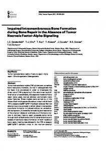
Frequent loosening of glenoid components is one of the major and challenging problems in total shoulder arthroplasty (Franklin et al. 1988, Lazarus et al. 2002). Radiolucent lines, which may be an indication of long-term loosening, have been observed at the bone implant interface even in up to 96 % of glenoid replacements (Lazarus et al. 2002). The consequence of component loosening can be dramatic, as a loosened component cannot always be replaced because of bone deficiencies (Cofield 1994). Therefore, there is a great clinical need to improve the fixation of glenoid components. Numerous all-polyethylene or metal-backed glenoid components, with keel- or peg-shaped backings, fixated either with or without cement, have been introduced in an attempt to reduce the high glenoid component loosening rate in total shoulder arthroplasty (Anglin et al. 2001, Cofield 1994, Neer 1974, Roper et al. 1990, Murphy et al. 2001). However, cemented glenoid components are limited by high stresses in the cement layer that cause damage (Lacroix et al. 2000) and osteolysis (Wirth and Rockwood Jr 1994), whereas cementless metal-backed components show problems with rapid polyethylene wear, component dissociation and pull out of the screws used for implant fixation (Bauer et al. 2002, Cofield 1994, Roper et al. 1990, Wallace et al. 1999, Archibeck et al. 2001). Therefore, improvement of glenoid component design is a relevant task. Two factors are important for bone ingrowth. One is an appropriate biocompatibility of the implant material (Bauer and Schils 1999) and the other is the initial stability of the implant; stable immediate (primary) fixation is a requirement for a successful secondary fixation by bone-ingrowth (Pilliar et al. 1986). With respect to implant material that can be used for glenoid backing, a promising material for bone-ingrowth is a trabecular metal named c (Implex, Allendale, USA). This is a highly porous (about 82%) Hedrocel� tantalum metal (Fig.2.1), with an apparent stiffness of 3.3 GPa, and porous structure, similar to cancellous bone (Zardiackas et al. 2001, Implex 2002). This material has been successfully used in acetabular cups, custom knee and tibial prostheses (Christie 2002). In canine models it has been reported that not only does bone apposition occur but osseointegration progressed through
2.2 Methods
7
the porous tantalum backing, leading to a rigid biomechanical fixation of the implant (Bobyn et al. 1999b). Application of porous tantalum is expected to solve the problem of polyethylene wear between the polyethylene layer and the metal backing, because polyethylene can be molded into the porous tantalum layer, rigidly fixing it to the backing which also facilitates making the whole component thinner. Hedrocel is known for one more advantage: the friction coefficient of 0.88 between this material and cancellous bone is higher than reported for traditional coated materials (0.50 - 0.66) (Fitzpatrick et al. 1997). This fact is expected to reduce the relative micromotions at the interface. The present chapter investigates the feasibility of bone ingrowth into the porous tantalum backing of a glenoid component. If ingrowth is to be achieved, then we also wanted to know what is the influence of primary fixation, elastic properties and friction coefficient of the backing on the ingrowth process.
Figure 2.1: Scanning electron microscopic image of Implex’s Hedrocel Trabecular Metal material (With permission from Implex, Allendale, New Jersey).
2.2 2.2.1
Methods Finite element model
To investigate bone ingrowth, a two-dimensional finite element modelling was used in conjunction with a mechano-biological algorithm to simulate osseointegration. Two-dimensional finite element models of three glenoid prosthesis design concepts were generated (Fig. 2.2). The glenoid bone region is divided into four domains (cancellous bone 1,2 and 3 and cortical bone; Lacroix and Prendergast 1997), that are modelled as isotropic materials with different
8
Chapter 2
Figure 2.2: Finite Element Meshes of three design configurations. A - design without pegs, B - design with non-parallel cemented pegs, C - design with parallel cemented pegs. 1 - Polyethylene, 2 - Porous Tantalum + Polyethylene, 3 - Porous Tantalum, 4 - Cancellous Bone 2, 5 - Cortical Bone, 6 Cancellous Bone 3, 7 - Cancellous Bone 1, 8 - Tantalum peg, 9 - cement. elastic properties (see Table 6.1). The glenoid components consist of three layers: a polyethylene surface layer, a porous tantalum layer, and fusion of both in between. One design is without pegs (Fig.2.A) and two have tantalum pegs cemented into the cancellous bone (Fig.2.2.B and Fig.2.2.C). These two pegged designs differ in the inferior peg configuration: one has parallel pegs and the other has non-parallel pegs. Mesh generation was performed using MSC Mentat (Version 2001, Palo Alto, USA). All domains were modelled by 8-noded isoparametric plain strain elements.
2.2.2
Material properties
The elastic properties for the glenoid bone regions (see Table 6.1) were taken from Orr et al. (1988) and Carter and Hayes (1977). The porous tantalum layer has a Young modulus of 3.3 GPa and Poisson ratio of 0.31 (Implex 2002). The average elastic properties of the porous tantalum filled with fibrocartilage or fibrous tissue were taken as properties of the porous tantalum alone, because the later is much stiffer than the filling soft tissues. The elastic properties of the porous tantalum filled with bone were determined from the micro finite element voxel model, developed for this purpose. The average permeability of porous tantalum, filled with bone, fibrous tissue and fibrocartilage is approximately determined based on the fact that perme-
2.2 Methods
9
ability of porous tantalum alone is very high compared to the permeability of the filling tissues. So, the average permeability of the whole material is mainly determined by the permeability of the filling tissue. It allows for the assumption that the total permeability can be estimated as permeability of the filling tissue multiplied by its fraction in the porous tantalum, with the porosity of porous tantalum being 0.82 (Implex 2002). Under these assumptions, multiplying the porosity of porous tantalum with the permeability of bone 3.7 × 10⁻¹³ m4 N −1 s−1 (Ochoa and Hillberry 1992), we obtain the average permeability of porous tantalum and bone 3.034 × 10⁻¹³ m4 N −1 s−1 . When we repeat the same procedure for fibrocartilage with permeability 5.0 × 10⁻¹⁵ m4 N −1 s−1 (Armstrong and Mow 1982) we obtain a permeability of 4.1 × 10⁻¹⁵ m4 N −1 s−1 , and in case of fibrous tissue with permeability 1.0 × 10⁻¹⁴ m4 N −1 s−1 (estimated by Prendergast et al. 1997 based on Armstrong and Mow 1982 and Levick 1987) the average permeability will be 8.2 × 10⁻¹⁵ m4 N −1 s−1 . In Marc 2001 porosity is a function of the Jacobian determinant of the deformation gradient tensor. However, the variation of the porosity is very small, as the poroelastic implementation in Marc 2001 assumes small strain theory. In the present study initial porosity of the porous tantalum with filled tissues was taken as porosity of porous tantalum alone, 0.82. The rationale for this is that tantalum is much stiffer than the filling tissues. Fluid compression modulus for all the tissues was taken as 2300 MPa (Anderson 1967). The coefficient of friction between bone and the porous tantalum layer was taken as 0.88 (Zhang et al. 1999). A Coulomb friction model was used. In order to investigate the influence of the material properties of the porous backing on the bone ingrowth process four additional simulations were performed. Two simulations for the configurations without pegs and with parallel pegs, investigated the case with zero friction coefficient. Another two simulations, for the configuration with parallel pegs, investigated the influence of Young modulus of the porous backing. Here, in the first simulation, Young’s modulus of the porous backing was taken ten times lower than the original (0.33 GPa). In this case it was assumed that when the backing gets filled with bone its stiffness will reach the stiffness of immature bone (1 GPa). In the second simulation, Young’s modulus of the porous backing was taken thirty times higher than the original (100 GPa). But in this case we assumed no change in the porous backing stiffness when bone grew in.
10
Chapter 2 Table 2.1: Elastic properties of materials, used in contact simulation. Material Young’s Modulus Poisson’s (GPa) ration Polyethylene 1.174 0.4 Porous Tantalum with Polyethylene 4.26 0.35 Porous tantalum 3.3 0.31 Porous tantalum with fibrous tissue 3.3 0.31 Porous tantalum with fibrocartilage 3.3 0.31 Porous tantalum with bone 5 0.35 Cancellous Bone 1 1.5 0.25 Cancellous Bone 2 0.4 0.21 Cancellous Bone 3 0.15 0.19 Cortical Bone 8 0.35 Tantalum 186 0.31 Cement 2.1 0.4
2.2.3
Boundary conditions
The applied loads correspond to an arm movement between 30o and 90o abduction in 2 seconds. The contact forces for 30o , 60o and 90o arm abduction (165.84, 325.85 and 392.95 N, Van der Helm 1994) are interpolated by a second order polynomial, thus creating a continuous dependence. In total 16 cycles of loading are simulated. Contact pressure was calculated based on Hertz theory of elastic contact of two spheres. The radius of the glenoid component was chosen as 30 mm, and humeral component 29.8 mm. All nodes on the medial border of the model are restrained as shown in (Fig.2.3). With respect to fluid flow, two boundary condition types were studied: zero pore pressure at the interface nodes of the porous tantalum layer which allows free fluid flow, and zero fluid flow, simulating a blocked interface. The side of the porous tantalum layer that faces the polyethylene layer is blocked by the impermeable polyethylene hence zero fluid flux was prescribed there.
2.2.4
Ingrowth model
Interface bonding Bone ingrowth into the porous tantalum backing is to a large extent analogous to bone fracture healing processes (for a review see Kienapfel et al. 1999). Following arthroplasty, a porous tantalum backing would become
2.2 Methods
11
Figure 2.3: Boundary conditions for the model. Left - schematic presentation of the glenoid component loaded by humeral head component. The humeral head is located according to 30o (I ) and 90o (II ) of arm abduction. Right - actual loading of the model: distributed pressure on the glenoid surface (1 ), clamped displacements of the medial border (2 ), free fluid flow at the boundary of the tantalum layer (3 ).
filled with granulation tissue. The first event that takes place at the interface is bone apposition (ingrowth into the surface) on the porous tantalum backing, this occurs by the intramembranous ossification mechanism. This results in bonding of the interface. During fracture healing, intramembranous ossification normally occurs in case of high mechanical stability and close proximity to existing bone (Bailon-Plaza and Van der Meulen 2001, Thompson et al. 2002), which is a source of osteoblasts and has rich vascularity. The interface area is the closest place to the existing bone and following, for instance, Spears et al. (2000), interface bonding can be simulated only if the relative interface micromotions do not exceed a certain threshold value. This approach has been adopted in the present research. For that purpose, pairs of adjacent nodes across the interface were identified and relative micromotions were defined as the maximum distance between the nodes of each pair during a loading cycle (Spears et al. 2000). Localized interface bonding is simulated by tying the displacements of the nodes thereby modelling a bonded interface. The interface bonding is simulated in regions of the interface where micromotions do not exceed a threshold value throughout one loading period. Due to the fact that no data was found in literature on this threshold value for porous tantalum, one of the lowest reported thresholds of 20μm was taken (Ramamurti et al. 1997). Despite the fact that this value is fairly low, it was chosen to give conservative ingrowth predictions.
12
Chapter 2
Mesenchymal cell migration After arthroplasty, mesenchymal cells migrate from the exposed bone surface across the interface into the porous tantalum backing. Mesenchymal cells migration from the interface into the porous layer is modelled by the linear diffusion equation: dc (2.1) = k∇2 c, dt where c is cell density, normalized with respect to “saturated” cell concentration and k is a diffusion coefficient. The coefficient of diffusion is selected in such a way that the complete mesenchymal cell coverage (c ≥ 0.95) in the porous tantalum layer would be achieved in 16 weeks. This is consistent with the time that was needed for bone ingrowth into porous tantalum backed acetabular cups (from clinical data, published by Implex 2002). Furthermore, it is assumed that migration of mesenchymal cells via the part of the interface that is bonded is allowed, whereas for the unbonded part it is not allowed. Consequently, as soon as a pair of the interface nodes becomes bonded, those nodes are assigned a “saturated” concentration of mesenchymal cells, while the rest of the boundary nodes are assigned a zero flux. Subsequent migration of cells into the porous tantalum layer is simulated by the linear diffusion equation (2.1).
Tissue differentiation inside the porous layer According to the mechano-regulation model for tissue differentiation proposed by Prendergast et al. (1997), absolute magnitudes of maximum shear strain γ and relative fluid/solid velocity ν are two biophysical stimuli that regulate tissue differentiation. Following this model, high levels of these stimuli (γ/a + ν/b > 3, a = 0.0375, b = 3μms−1 - constants, determined by Huiskes et al. (1997) based on an animal experiment) favor differentiation of mesenchymal cells into fibroblasts, intermediate levels (γ/a + ν/b > 1 and γ/a + ν/b < 3) favor chondrocytes differentiation and low levels (γ/a + ν/b < 1) - osteoblasts. In the current simulation, the tissues inside the porous tantalum layer are modelled as biphasic materials. Shear strain and fluid velocity are calculated from biphasic simulation and, subsequently, differentiation of mesenchymal cells is simulated. Consequently, tissue type at the integration point of the porous backing is determined using the absolute magnitudes of the shear strain and fluid velocity. The subsequent tissue fraction is taken equal to the normalized mesenchymal cell concentration. This comes from the assumption that the quantity of the newly produced tissue is directly
2.2 Methods
13
dependent on the concentration of the mesenchymal cell in this point. It is also assumed that the cells of this newly created tissue can be replaced by the equal concentration of the cells of another phenotype if the mechanical environment changes. Hence, in the model, we do not make a distinction between the phenotype of the cells, as we assume that all of them, like the mesenchymal cells, have a potential to produce tissue type, dictated by the mechanical environment in the given point. Thus, the initial granulation tissue and another tissue might co-exist simultaneously in one integration point. A rule of mixtures is used to calculate the material properties in those cases (Lacroix and Prendergast 2002b). According to this rule, for instance, Young modulus of the integration point is calculated as a sum of products of Young moduli of the co-existing tissues and their volume fractions.
2.2.5
Solution procedure
The simulation is performed using MSC Marc (Version 2001, Palo Alto, USA). For the first configuration (Fig. 2.2, A), the whole bone-implant interface was assumed as unbonded. In the second and the third design configurations the prosthesis was initially connected to the bone via cemented pegs, while the rest of the interface was modelled as initially unbonded. Each simulation consists of three parts: contact analysis, biphasic analysis and diffusion analysis. In Fig.2.4 a summary of the analysis is given. Contact analysis of the glenoid bone with the prosthesis calculates interface micromotions and displacements of the porous layer boundary. Biphasic analysis of the porous tantalum layer calculates biophysical stimuli. Diffusion analysis of the porous tantalum layer calculates concentration of mesenchymal cells. The update of the material properties inside the porous layer for both contact and poroelastic simulation during every loading cycle is performed gradually, during the first tenth of the loading cycle time. All simulations are coupled. The contact simulation starts with unbonded bone implant interface and granulation tissue inside the porous layer. The calculated interface micromotions are used to decide which interface nodes are to be bonded. The list of the newly bonded nodes is passed to the diffusion simulation, where they become sources of mesenchymal cells. Displacements of the boundary nodes of the porous layer are also calculated in the contact simulation and passed to the poroelastic simulation. There they are used as kinematic boundary conditions. The poroelastic simulation calculates fluid velocity and tissue maximum shear strain, that are used to decide which tissue type should appear in an integration point. Given this information and the concentration of mesenchymal cells, calculated in the diffusion simulation, material properties are calculated and passed to the contact simulation.
14
Chapter 2
fluid flow
Tissue shear strain
Figure 2.4: Solution procedure. Initially, the interface is unbonded and there are no mesenchymal cells in the porous tantalum layer. After application of the loading, mesenchymal cell concentration, interface micromotions and biophysical stimuli are calculated. The tissue properties are determined for each integration point of the porous layer depending on its position in the tissue-differentiation diagram (under Update of the material properties due to tissue differentiation) and updated in both poroelastic and contact simulations. The pairs of interface nodes are bonded depending on the level of the calculated micromotions. Bonded nodes are assigned “saturated” concentration of mesenchymal cells. After all the updates the next analysis cycle is started.
There is a difference in time scale of the analysis in the simulation loop. The migration of mesenchymal cells in the diffusion analysis lasts for one week before the sources of mesenchymal cells are updated by the contact analysis whereas one arm movement lasts for 2 seconds, which is a time period of the loop depicted in Fig.2.4. As it was mentioned before, 16 weeks were needed to achieve bone ingrowth in an acetabular cup (Implex 2002). Therefore, 16 weeks of mesenchymal cell migration and 16 arm movements were simulated. Each simulated movement should be seen as a “characteristic” movement for the current week of the cell migration simulation. A parameter study to determine the influence of constants a and b (see
2.3 Results
15
Section 2.3) and the inhibiting micromotions threshold level was performed by varying these values along the baseline of the above mentioned magnitudes. This parameter study was performed only with the original material properties of the porous tantalum (Young modulus 3.3 GPa, friction coefficient 0.88).
2.3
Results
Boundary conditions without free fluid flow at the bone-implant interface resulted in complete interface bonding and full bone ingrowth for both configurations with pegs. Since the worst case scenario is thought to be more interesting for the ingrowth prediction, from here on we report only on the results obtained with boundary conditions which allowed fluid flow at the interface. Lack of primary fixation is predicted to have a substantially negative influence on bone ingrowth into the porous layer of the design configuration without pegs. Very high micromotions (Fig. 2.5) resulted only in a partial interface bonding (Fig. 2.7). Introduction of non-parallel cemented tantalum pegs in the second design configuration stabilized the prosthesis and interface bonding is predicted everywhere, except the area above the superior peg where micromotions even increase as bonding of the rest of the interface propagates (Fig. 2.5, the graph). The situation with the third design is similar, but peg orientation causes a more uniform distribution of the micromotions (Fig. 2.5 and Fig. 2.6, C). As a result, complete bonding of the interface is achieved. Reducing the stiffness of the porous tantalum layer to 0.33 GPa resulted in higher interface micromotions (Fig. 2.6, C), while increasing it to 100 GPa, causes micromotions to decrease (Fig. 2.6, C). Lack of friction resulted in almost threefold increase of micromotions for the design without primary fixation, although this effect was prominent only in the top part of the interface, where the prosthesis came in contact with bone (Fig. 2.6,A area marked by a circle). Absence of friction caused very little effect on the design with parallel pegs, where micromotions increased less then 10 percent (not plotted). Bonding of the interface allows migration of mesenchymal cells from the interface into the porous layer and their subsequent differentiation into other cells depending on the biophysical stimuli. Partial bonding of the interface (Fig. 2.7) and low biophysical stimuli inside the porous layer resulted in partial bone ingrowth for the first design configuration (Fig. 2.8). Although pegs facilitated greater area of interface bonding for the second configuration, strain concentration near the top peg resulted in a little amount of
16
Chapter 2
Figure 2.5: Micromotions at the interface during the ingrowth. The graph shows micromotions magnitude for the node specified by an arrow during the simulated arm movements for the first four weeks. cartilagineous tissue, that did not ossify till the end of the simulated time. Parallel pegs, on the contrary, resulted in complete bone ingrowth. However, some amount of cartilage appeared during the simulation, but it was completely replaced by endochondral ossification. Decreasing stiffness of the porous layer to 0.33 GPa increased the biophysical stimuli, i.e. a substantial
2.3 Results
17
Figure 2.6: Micromotions before the ingrowth (the first week) at 30o arm abduction. A - configuration without primary fixation with and without friction. B - configuration with non-parallel pegs with original elastic and friction properties. C - configuration with parallel pegs with soft (0.33 GPa), original (3.3 GPa) and stiff (100 GPa) backing.
part of the backing was filled with cartilage and fibrous tissue (Fig. 2.8). Increasing the stiffness to 100 GPa resulted in complete bone differentiation via the intramembranous ossification mechanism. The parameter study showed little sensitivity of the simulation to the moderate (25 %) variation of constants a and b (variation of b had more influence on the simulation). Increasing the inhibiting micromotion threshold to 30 μm caused more rapid interface bonding for the configuration with pegs
18
Chapter 2
Figure 2.7: Interface bonding. Results correspond to the original material properties of the porous tantalum backing (Young modulus 3.3 GPa, friction coefficient 0.88). and also a complete interface bonding for the configuration with non-parallel pegs.
2.4
Discussion
The aim of this numerical study was to establish whether or not bone ingrowth in porous tantalum backed glenoid components is likely under physiological loading. If the ingrowth is to be achieved, then we also wanted to know what is the influence of primary fixation and material properties of the backing on bone ingrowth. In order to simulate bone ingrowth, several assumptions were necessary. First, modelling of ingrowth at the bone-implant interface was done by tying the displacements of the interface nodes. In general, this might lead to an overestimation of the strength of the newly formed interfacial bonds and
2.4 Discussion
19
Figure 2.8: Tissue types and their fractions inside the porous tantalum layer. The bottom row shows tissue types inside the third design configuration with the reduces stiffness of the backing (0.33 GPa).
subsequent overestimation of the overall area of ingrowth. However, using this approach for an acetabular cup, Spears et al. (2000) predicted ingrowth patterns comparable with histological data for dogs. Simmons and Pilliar
20
Chapter 2
(2000) tried to estimate the probability of interface ingrowth by modelling the interface with elements which properties were obtained by a homogenization procedure applied to a detailed interface model. However, their model was linear, unlike the non-linear procedure of contact with friction that is used in the present study. The second simplification was the use of 2D instead of 3D models. There is no doubt that the latter would give a more realistic view on the stress-strain situation. It is expected that the plane strain assumption will cause some underestimation of the interface micromotions, the low value of the micromotion threshold chosen, that inhibits bone ingrowth, is expected to compensate for this underestimation. Third, the time period for the update of the material properties of the backing and the interface nodes bonding was one week. Thus we assumed that the average time period necessary for initial tissue formation is one week. This is roughly consistent with the experimental study of Le et al. (2001), who observed fibroblasts differentiation 3 days after bone fracture, cartilage formation in 5 to 7 days, and woven bone in 14 days. Also Bobyn et al. (1999a) observed bonded interfaces and 13 percent bone ingrowth in porous tantalum implant two weeks post-operatively. The last important assumption adopted here, involves the usage of the thresholds from Huiskes et al. (1997) for the tissue differentiation model of Prendergast et al. (1997). We anticipate, that those values might vary from species to species or even among individuals. However, parameter studies on those thresholds performed in our study and by Lacroix and Prendergast (2002b) show that the variation of those thresholds does not greatly change the tissue differentiation patterns. Using these thresholds, Lacroix and Prendergast (2002b) successfully predicted the main stages of a fracture healing process and Geris et al. (2004) predicted the main stages of tissue differentiation inside a bone chamber implanted into a rabbit’s leg. We cannot provide direct experimental validations of the simulation results due to the fact that we are not aware of clinical data on porous metalbacked glenoid components. However, some of the features of the simulated ingrowth resemble ingrowth patterns observed in other implants. For instance, the simulation predicts that the bonding of the interface starts near the pegs (Fig.2.7). This can be compared with the results for porous-coated tibial components of total knee replacements where it was found that bone ingrowth occurred within and near the fixation pegs but was variable elsewhere (Sumner et al. 1995, Kienapfel et al. 1996). There are several experimental studies on bone ingrowth into porous tantalum (Bobyn et al. 1999a, Bobyn et al. 1999b, Macheras et al. 2000, Sidhu et al. 2001, Zou et al. 2001). Sidhu et al. (2001) show how lack of initial stability can inhibit bone ingrowth into the implant. The same conclusion can be drawn from our results for the first
2.4 Discussion
21
design configuration (Fig.2.8). Bobyn et al. (1999b) show that, even if the interface is partially bonded, bone ingrowth does not take place via the unbonded part of the interface. This aspect was also predicted by the simulation for the second design configuration. This observation is fully consistent with our assumption that precursor cells do not migrate via the unbonded part of the interface, thus bone ingrowth inside an unbonded prosthesis is inhibited. Finally, Bobyn et al. (1999a) show that, if primary fixation is provided, the ingrowth kinetics resembles the patterns produced by the simulation (configuration with parallel pegs, Fig.2.8). The main difference with our results is that Bobyn et al. (1999a) observed rather sparse ingrowth in the part of the porous tantalum area that is inserted into cancellous bone. At the same time, the zone adjacent to the cortical bone achieved much higher bone density. One possible explanation for that is that we did not simulate bone resorption. Lacroix and Prendergast (2002b) managed to predict resorption of the external callus during fracture healing simulation when the biophysical stimuli were very low. But analyzing the magnitude of the stimuli inside the porous layer in our simulation, we predict that only very stiff porous backing (100 GPa) would lower the stimuli’s magnitude, consequently bone resorption could become important. But even in this case, the area where those low stimuli were observed, occupied only 10 percent of the porous tantalum layer. It should be noted, that Lacroix and Prendergast (2002b) also could not predict resorption of the internal callus and concluded that tissue differentiation in the medullary cavity must be guided by biological rather than mechanical factors. The last difference between the experiments and our results is that we predicted a small amount of cartilage during the intermediate stage of the ingrowth. Based on the current simulation results for the interface micromotions (Fig. 2.5 and Fig. 2.6), we can conclude that, for the considered design configurations, a stiffer porous backing would be more advantageous. Worth mentioning that there are studies that show the opposite effect, i.e. that the lower the stiffness of the implant, the lower the peak interface micromotions (see for instance Simon et al. 2003). Hence, it can be concluded, that the optimal stiffness of the ingrowth type material depends on the specific orthopaedic application. Our study also shows that if primary fixation is provided, the friction at the bone-implant interface hardly influences the interface micromotions. Potentially, this observation could widen the choice of implant materials for implant designers. It should be added, that the designers of glenoid prostheses should not use every chance to reduce the interface micromotions, but rather come up with such initial fixation that will produce a reasonably uniform distribution of the interface micromotions. Intuitively, one might think that the longer lower peg in the design with non-parallel pegs
22
Chapter 2
should cause lower micromotions and, subsequently, faster interface bonding than for the design with parallel pegs. And, indeed, the micromotions around the lower peg are sufficiently lower than for the design with parallel pegs (Fig. 2.6,B). But this longer peg causes imbalance in the micromotion distribution, hence boosting micromotions in the least restrained part of the interface, above the top peg. The design with parallel pegs produces a more uniform micromotion distribution, although on average the micromotions are higher than in the case of the design with non-parallel pegs. But this appears to be unimportant as long as the produced micromotions are still lower than the threshold value. Worth mentioning that by increasing the inhibiting micromotions threshold the differences between interface bonding patterns for the two configurations with pegs vanishes (parametric study). Nonetheless the parallel pegs configuration still performs better. The simulation also indicates that failure of bone differentiation inside the backing would start at very low stiffness magnitudes of the porous materials, used for the backing. The authors also performed several simulations with stiffness magnitudes of the backing between 0.33 GPa and 3.3 GPa, but only at 0.33 GPa cartilage and fibrous tissue persisted till the end of the simulation. In conclusion, the simulation predicts that primary stability of a glenoid component with porous tantalum backing can be reached, and mechanical conditions, that allow complete bone ingrowth into the porous tantalum layer, can be created. In particular, it was predicted that a design with parallel cemented pegs could confer sufficient primary stability allowing bone ingrowth at the implant interface.
Chapter 3 Poroelastic formulation for finite element modelling of hydrated tissues Abstract Biological tissues like skin, cartilage or artery walls contain large amounts of water and are subjected to large deformations. This results in complex nonlinear time dependent behavior. A finite element formulation for simulation of poroelastic media is proposed. The formulation is based on a mixed formulation with both small and finite strain assumptions. The formulation is implemented as a user element in the commercial FE package MSC Marc. Consequently, this allows an easy enhancement of the formulation with material models that are already available in MSC Marc. Moreover, usage of MSC Marc’s features such as parallel computations, sub-structuring, contact, etc. is possible. As a result, nonlinear elastic or plastic behavior can be added to the poroelastic formulation at no additional implementation costs. The implementation of the proposed formulation is validated with an existing small strain poroelastic Marc element and study on a poroelastic finite strain problem, known from literature.
3.1
Introduction
Human tissues contain a large fraction of fluid that strongly influences their mechanical behavior. Consequently, many researchers used poroelastic theory to model these tissues. For instance, Mow et al. (1980) was the first to apply poroelastic theory for modelling articular cartilage. Oomens and Van 23
24
Chapter 3
Campen (1987) used a mixture approach to model skin. Poroelastic theory was used for modelling bone tissue (see Cowin (1999) for a review). Most of the biomechanical problems require modelling of many physical phenomena at the same time. For instance, this thesis discusses a problem where contact mechanics is combined with poroelastic behavior of tissues and migration of cells, modelled by diffusion equations. Also geometry of the problems considered in biomechanics might be very complex. In most cases, geometries are derived from medical images, such as Computer Tomography scans or Magnetic Resonance Imaging techniques. Due to this complexity, usage of “home”- made Finite Element software packages in biomechanics is rather limited, as it requires too much development, not related to biomechanics itself. Even most of the geomechanics software packages that include finite elements for poroelastic theory are too specialized to be used in biomechanics. General software packages like TNO Diana (Delft, The Netherlands) or MSC Marc (Palo Alto, USA) do include models for poroelasticity, but these are not fully suitable for biomechanical problems. For instance, the poroelastic formulation used in MSC Marc does not include geometrical non-linearity, while both packages use a formulation resulting in non-symmetric stiffness matrix, which increases the computing time and the amount of memory, that needs to be allocated for matrix storage. In this study, we attempt to combine multifunctional, commericaly available FEM software, like MSC Marc, with a custom-implemented poroelastic model, which is particulary suited for biomechanical applications. The proposed formulation is implemented as a user-defined element in MSC Marc. The main features of the element are its tetrahedral shape, symmetric stiffness matrix and finite strain formulation. Due to the fact that the element is based on a mixed formulation, the degrees of freedom are displacements of the solid phase and fluid pressure.
3.2
Theory
The basic assumptions of the poroelastic theory are outlined in Mow et al. (1980). The main assumption of the theory is that any poroelastic (also called biphasic) domain can be viewed upon as a superposition of two single continua. Each of the continua follows its own motion and at any time t each position x in the poroelastic domain is occupied by two different particles, each particle corresponding to one constituent denoted by α. Here α = f corresponds to the fluid phase and α = s denotes solid. Due to the fact that each constituent is modelled as a continuum, prop-
3.2 Theory
25
erties which are defined per unit area or volume have a “true” and an “apparent” value. The true volume is the volume that constituent α occupies physically. The true density ρα∗ is defined as the mass of constituent α divided by the true volume Vα of constituent α. The apparent density ρα is the mass of phase α divided by volume V of the whole poroelastic domain, hence: Vα α α α α ρ = n ρ∗ with n = . (3.1) V It should be noticed, that when material constituents intermingle on the molecular level, a volume fraction has no true physical meaning. In that case, the apparent densities are more suitable as independent variables. Given these definitions, other important assumptions can be introduced. The fluid inside the poroelastic domain is assumed to be only slightly compressible and inviscid (Newtonian), however, we assume the existence of drag forces that oppose the flow of the fluid through the solid phase. The material of the solid phase is assumed to be incompressible, i.e. its true density ρs∗ = const. However, this does not imply the incompressibility of the solid phase in the apparent sense, as the porosity of the solid phase can change due to deformation, hence ρs ≡ ns ρs∗ �= const. The position x of a particle of constituent α is a function of time as well as its original or reference position vector X, i.e. xα = φ α (Xα , t).
(3.2)
The velocity of the particles is defined as vα =
φα dφ . dt
(3.3)
In order to define the material time derivative of a physical property, we have to take into account which constituent is our relevant reference. If the observer wishes to move along with constituent α, the material time derivative of a property ψ = ψ(x, t) is given by ∂ψ d(α) ψ = + vα · ∇ψ. dt ∂t
(3.4)
For each constituent we can define a deformation tensor Fα =
∂xα . ∂Xα
(3.5)
Because each constituent is regarded as a continuum, following its own motion, it is possible to derive balance laws for each constituent. These balance
26
Chapter 3
laws are the same as those for a single-phase material, except for so-called interaction terms. The later arise from the presence of other constituents. Using (3.4), we can derive the local balance of mass for the constituent α ∂ρα + ∇ · (vα ρα ) = cα ∂t
(3.6)
The quantity cα is an interaction term that represents the mass supply from the other constituents. This term is important for chemically reacting media. The balance of the poroelastic medium as a whole leads to cs + cf = 0.
(3.7)
We assume no chemical interaction between the constituents, hence cα = 0. The governing equations for the poroelastic model can now be derived from the principle of virtual power. First we define a functional space for the test functions: � � (3.8) δvjα U0 , U0 = δvjα | δvjα C0 (X), δvjα = 0 on Γvj , where Γvj is a part of the boundary with kinematic boundary conditions. With this selection of the space of test functions δvα the integral over the kinematic boundary vanishes, and the only boundary integral is the one for the traction boundary. The test functions are also called virtual velocities. With the above test functions, we can write the principle of virtual power as δPα = δPαint + δPαkin − δPαext = 0 ∀δvi U0 ,
(3.9)
where δPα is the rate of total virtual work or the total virtual power of constituent α, δPαint - the rate of internal virtual work or the virtual internal power of constituent α, δPαkin - the virtual kinetic power of constituent α , δPαext - the virtual external power of constituent α. The virtual kinetic power δPαkin of constituent α is given by � kin δvα · v˙ α ρα dV, (3.10) δPα = V
where v˙ α is the acceleration of the α phase. The behaviour of the solid phase is assumed to be elastic, therefore the virtual internal power of the solid phase is essentially the rate of mechanical energy, stored in the solid. Hence, � int δDs ∗ : σ s∗ dV s , (3.11) δPs = Vs
3.2 Theory
27
where σ s∗ is a true stress in the solid, Ds∗ is the true deformation rate tensor s s i s ∗ = 12 ( ∂δv + δv∂x∗i j ). The aim of the above for the solid phase and δD∗ij ∂xj derivations is to obtain the governing equations for the whole poroelastic domain. Therefore, the integral over V s domain, which is a true geometry of the porous solid in (3.11), should be replaced with an integral over the whole poroelastic volume V . In order to do this, we replace the true stress in the solid phase σ s∗ with σ sE , which is a Cauchy stress tensor for the solid phase in the apparent sense. Similarly, we replace the true deformation rate Ds∗ with Ds - a deformation rate of the solid phase in the apparent sense. In fact, this step should be seen as an averaging procedure, where an inhomogeneous material is replaced by a homogeneous material which is capable to store the same amount of mechanical energy per unit volume under the equal load. Hence we can write � � int s s s δD ∗ : σ ∗ dV = δDs : σ sE dV. (3.12) δPs = Vs
V
Since we have assumed that the fluid is slightly compressible, it can also store mechanical energy. The fluid was assumed to be Newtonian, hence its true stress is σ f∗ = −pI. In case of fluid it is easy to see that the apparent fluid stress will be the the same true stress scaled with the fraction of the fluid σ f = −nf pI. Hence, the internal virtual power for the fluid phase is � int δPf = δDf : −nf pIdV. (3.13) V
The virtual external power for both phases is given by � � � ext α α α α α δPα = δv · ρ f dV + δv · Π dV + δvα · tα dΓ + δPαp , (3.14) V
V
Γtα
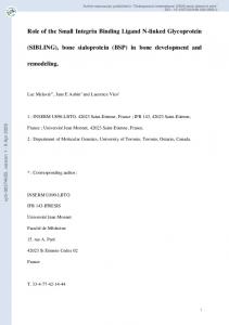
where f α is a body force per unit mass, Π α - diffusive resistance due to the relative flow between two different phases, tα - is a traction force applied on the Γtα part of the boundary, δPsp - is a rate of virtual work, performed by the fluid pressure on the solid phase (see Fig. 3.1) and δPfp - is a rate of virtual work, performed by the hydrostatic expansion of the solid on the fluid. Following the conventions of the poroelastic theory, we assume that the diffusive drag Π α is proportional to relative velocity between the two phases: Π α = K(vβ − vα ) where α = f, s and β = s, f
(3.15)
Here K - is a diffusive drag coefficient. It follows from (3.15) that Π f + Π s = 0.
(3.16)
28
Chapter 3
Figure 3.1: Schematic representation of a poroelastic medium at the microlevel. The medium consists of the solid part represented by grains which are embedded in the fluid that can move between the grains. The movement of the fluid causes the appearance of the drug forces Π f and Π s acting at each of the constituents. The fluid pressure p also contributes to the deformation of the solid phase by rearranging the solid grains. Similarly to (3.13), it can also be shown that the rate of virtual work, performed by the fluid pressure on the solid phase is � δPsp
=
δDs : ns pIdV .
(3.17)
V
Unlike (3.13) we do not have a minus sign in front of the right hand side of (3.17) because it represents an external power, while (3.13) is an internal power. The interpretation of the above power is the following. Although the solid phase is considered to be incompressible, fluid pressure still can perform work on the solid skeleton, which results in deformation. The reason is that the fluid pressure is not uniformly applied to the entire surface of the solid skeleton due the presence of fluid pressure gradients and due to the fact that the fluid pressure is not applied to the part of the skeleton surface that coincided with the surface of the poroelastic domain. As the solid phase is incompressible, the hydrostatic expansion of the solid phase is zero. As a result the rate of the work, performed by the hydrostatic expansion of the solid on the fluid is also zero δPfp = 0.
(3.18)
3.2 Theory
29
Now, substituting all the calculated virtual power contributions into the principle of virtual power (3.9) and regrouping some terms, we obtain � � s s s σ E − n pI)dV + δD : (σ δvs · v˙ s ρs dV = V �V � � s s s s s = δv ρ f dV + δv Π dV + δvs ts dΓ, (3.19) V
�
V
Γts
�
f
δD : (−n pI)dV + δvf · v˙ f ρf dV = V �V � � f f f f f = δv ρ f dV + δv Π dV + δvf tf dΓ. f
V
V
(3.20)
Γtf
In the above we introduce a notation σ s = σ sE − ns pI and substitute −nf pI with σ f . Although, in the true sense, fluid pressure is an external load for the solid phase, it can be seen as as the part the solid stress in the apparent sense. In order to obtain the strong form of the poroelastic theory, the derivatives of the test functions must be eliminated from (3.19) and (3.20). This is accomplished by using the derivative product rule, which gives � � 1 � ∂δvα � ∂δvα �T � α α α : σ dV = δD : σ dV = + ∂x ∂x V V 2 � � α α = ∇ · (δv σ )dV − δvα ∇ · σ α dV . (3.21) V
V
We now apply Gauss’s theorem to the first term on the right hand-side of (3.21): � � � α α α α ∇ · (δv σ )dV = δv (n · σ )dΓ = δvα (n · σ α )dΓ, (3.22) V
Γ
Γtα
where Γ is the boundary of the poroelastic domain, Γtα is the traction boundary for constituent α and n is the external normal on the surface element. The second equality follows from (3.8). Substitution of (3.21) and (3.22) into (3.19) and (3.20) leads to � � � (3.23) δvs v˙ s ρs − ∇ · σ s − ρs f s − Π s dV + V � � � + δvs (n · σ s ) − ts dΓ = 0, Γts
30
Chapter 3 �
� � δvf v˙ f ρf − ∇ · σ f − ρf f f − Π f dV + V� � � + δvf (n · σ f ) − tf dΓ = 0.
(3.24)
Γtf
Based on the fundamental theorem of the virtual calculus all of the terms contained in each square bracket of (3.23) and (3.24) should be equal to zero. A set of governing equations for the poroelastic model can now be derived: Momentum equations v˙ s ρs − ∇ · σ s − ρs f s − Π s = 0,
(3.25)
v˙ f ρf − ∇ · σ f − ρf f f − Π f = 0.
(3.26)
n · σ s = ts on Γts ,
(3.27)
n · σ f = tf on Γtf .
(3.28)
σ s = σ sE − ns pI,
(3.29)
σ f = −nf pI.
(3.30)
Boundary conditions
Here we recall that
Hence, the traction boundary conditions can be presented as σ sE − ns pI) = ts on Γts , n · (σ |tf | on Γtf . nf The Cauchy stress of the solid phase σ sE can be presented as p = p (x) ≡ −
σ sE = Fs · τ sE · (Fs )T ,
(3.31) (3.32)
(3.33)
where τ sE is the second Piola-Kirchhoff stress tensor. For isotropic linear elastic material, τ sE is given by τ sE = λs tr(Es )I + 2μs Es ,
(3.34)
where λs and μs are the Lam´e elasticity constants and 1 Es = (FsT · Fs − I) 2
(3.35)
is the Green strain tensor. In case of large deformations, it is common to replace the isotropic linear law (Hooke’s law) with Neo-Hookean material model, where τ sE is given by � � (3.36) τ sE = λs lnJC−1 + μs I − C−1 .
3.2 Theory
31
Here C = FT · F is the right Cauchy-Green deformation tensor and J = det(F) - Jacobian of the transformation between the current and the reference configurations. Using the fact that nf + ns = 1 and Π f + Π s = 0, the two momentum equations, (3.25) and (3.26), can be summarized as a total momentum equation for poroelastic model: ˙ − ∇ · σ − ρf = 0. vρ Here, σ=
α
f=
(3.37)
σ α = σ sE − pI,
(3.38)
ρα f α /ρ,
(3.39)
α
and the density average velocity v is defined as
ρα vα /ρ. v=
(3.40)
α
In biomechanical applications, the state of the poroelastic domain is mainly determined by its deformation, while both gravity and inertia effects are considered to be negligible, i. e. f α ≈ 0 and v˙α ρα ≈ 0. Given these assumptions it is interesting to notice that if we substitute (3.15) and (3.30) into (3.26), it will transform into Darcy’s law: nf (vf − vs ) = −
(nf )2 (∇p). K
(3.41) f 2
In the conventional notation of Darcy’s law it is set (nK) = μκ , where κ - is a permeability of the solid phase and μ - viscosity of the fluid. After the above derivations, we can obtain the mass balance equation for the whole poroelastic domain. State equations for the fluid phase have been given by Fernandez (1972) as ρf∗ = ρf∗0 e−βf T +Cf (p−p0 ) ,
(3.42)
where the subscript 0 indicates an initial steady state at standard conditions, βf is the thermal expansion coefficient and Cf is the compressibility coefficient. By retaining the first-order series expansion of (3.42) we obtain: ρf∗ = ρf∗0 [1 − βf T + Cf (p − p0 )].
(3.43)
32
Chapter 3
Hence we can write:
∂ρf∗ 1 f ∂p ρ = , ∂t Kf ∗0 ∂t
(3.44)
where Kf = 1/Cf is the bulk modulus of the fluid. Now, taking into account that ρα = nα ρα∗ and cα = 0, mass balance equations (3.6) read: ρα∗
∂nα ∂ρα + nα ∗ + nα ρα∗ ∇ · vα + vα · ∇(nα ρα∗ ) = 0 ∂t ∂t
(3.45)
Substituting (3.44)s into (3.45), taking into account the incompressibility of ∗ = 0) and neglecting the gradients of densities (Lewis and the solid phase ( ∂ρ ∂t Schrefler 1998) we obtain ∂ns + ns ρs∗ ∇ · vs = 0, ∂t
(3.46)
nf f ∂p ∂nf + + nf ρf∗ ∇ · vf = 0 ρ ∂t Kf ∗0 ∂t
(3.47)
ρs∗ ρf∗
Now we divide (3.46) and (3.47) with ρs∗ and ρf∗ , respectively, and take into account that
ρf∗0 ρf∗
≈ 1 (Lewis and Schrefler 1998). We obtain then ∂ns + ns ∇ · vs = 0, ∂t
(3.48)
∂nf nf ∂p + + nf ∇ · v f = 0 ∂t Kf ∂t
(3.49)
The equations (3.48) and (3.49) are now added together and here we can use s f the fact that nf + ns = 1 (hence ∂n + ∂n = 0). We obtain ∂t ∂t nf ∂p + nf (∇ · vf − ∇ · vs ) + ∇ · vs = 0 Kf ∂t
(3.50)
The numerical implementation, presented in the following paragraph, is based on a mixed formulation. The later models the behaviour of the poroelastic domain via the displacement field of the solid and the fluid pressure. Consequently, we have to eliminate the fluid velocity from the governing equations. In (3.50) the fluid velocity can be eliminated by using Darcy’s law, where we also assume that nf (∇ · vf − ∇ · vs ) = − μκ [∇p]. Hence, the mass balance equation for the whole poroelastic domain is �κ � nf ∂p + ∇ · vs − ∇ · (∇p) = 0. Kf ∂t μ
(3.51)
3.3 Numerical implementation
33
Under the assumption of negligible inertia forces and lack of gravity, the momentum equation for the poroelastic domain (3.37) simplifies into: ∇ · σ = 0.
(3.52)
In order to complete the set of the governing equations, initial and boundary conditions must be defined. The initial conditions define the complete solution at time t = t0 : us |t=t0 = us0 (x), p|t=t0 = p0 (x) on V
(3.53)
Dirichlet’s type boundary conditions are imposed in the form of applied displacements on parts of the boundary, denoted as Γu : us = gs (x) on Γu .
(3.54)
The fluid influx is defined as the fluid quantity, that crosses a unit surface of the boundary of the poroelastic domain during a unit of time. Based on this definition, the fluid influx is ρf∗ nf (vf − vs )T · n. Here, we can eliminate fluid velocity using Darcy’s law. In this case, the fluid flux boundary condition is prescribed as q f (x) κ on Γqf , − (∇p)T · n = f μ ρ∗
(3.55)
where Γqf is the part of the boundary where fluid flux is prescribed. The equilibrium equation (3.52), the mass balance equation (3.51), the initial and boundary conditions (3.31), (3.32),(3.53), (3.54) and (3.55) together with the constitutive equations (3.34) or (3.36) are the governing equations of the presented poroelastic theory, which fully define the behavior of the poroelastic domain under the proposed assumptions.
3.3
Numerical implementation
The boundary value problem (3.51), (3.52), (3.31), (3.32), (3.54),(3.55) is solved using the mixed formulation presented below. The formulation presented by Lewis and Schrefler (1998) is taken as a basis for the development of a new formulation. Voigt notation for stress and strain is used: σ = {σxx , σyy , σzz , τxy , τyz , τzx }T
(3.56)
E = {Exx , Eyy , Ezz , 2Exy , 2Eyz , 2Ezx }T
(3.57)
34
Chapter 3
With the Voigt notation the equilibrium (3.52) can be presented as LT σ = 0,
(3.58)
where L is the differential operator defined as ⎡ ∂ ⎤ 0 0 ∂x ⎢ 0 ∂ 0 ⎥ ⎢ ⎥ ∂y ⎢ 0 0 ∂ ⎥ ⎢ ⎥ L = ⎢ ∂ ∂ ∂z ⎥ . ⎢ ∂y ∂x 0 ⎥ ⎢ ∂ ⎥ ∂ ⎣ 0 ∂z ⎦ ∂y ∂ ∂ 0 ∂x ∂z
(3.59)
The stress tensor can also be presented as: σ = σ sE − m · p,
(3.60)
where mT = {1, 1, 1, 0, 0, 0}T and σ sE is rewritten in Voigt notation (3.56). A finite element formulation is derived using the weighted residual method (see Lewis and Schrefler 1998). For that purpose, lets multiply (3.58) with arbitrary functions w from H01 (where H01 is a standard Sobolev space, which implies that the function can be integrated along with its first derivatives and vanishes on the boundary) and integrate over V : � wT (LT σ )dV = 0 (3.61) V
If we use the fact that wT (LT σ ) = LT (wT σ )−(Lw)T σ , and take into account Green’s theorem, (3.31) and (3.32), which gives us � � � T T T σ · n)dΓ = L (w σ )dV = w · (σ wT tdΓ, (3.62) V
Γ
Γt
(3.61) can be presented as: � � T (Lw) σ dV = wT tdΓ. V
Here
(3.63)
Γt
⎡ ⎢ ⎢ ⎢ n=⎢ ⎢ ⎢ ⎣
⎤ nx 0 0 0 ny 0 ⎥ ⎥ 0 0 nz ⎥ ⎥, ny nx 0 ⎥ ⎥ 0 nz ny ⎦ nz 0 nx
(3.64)
3.3 Numerical implementation
35
where nx ,ny and nz are the components of the unit vector, normal to the boundary. We also combined the traction boundary conditions applied to the solid and the fluid phases for brevity of the notation. Now, lets assume another set of weighting functions w H01 . By multiply (3.51) with w and integrating it over V we obtain: � � nf ∂p �κ �� T w · + ∇ · vs − ∇ · (∇p) dV = 0. (3.65) Kf ∂t μ V Now, as in case of the equilibrium equation, taking into account that � � � � � �κ κ T T κ (∇p) − (∇w)T ( (∇p)) (3.66) w · ∇ · (∇p) = ∇ · w μ μ μ and � V
� � � � � � � � � � qf T κ T κ (∇p) dV = (∇p) · ndΓ = ∇· w w wT dΓ, (3.67) μ μ ρf Γ Γqf
and noticing that ∇ · vs = mT Lvs , (3.65) can be presented as � � � f � � T κ T T s T n ∂p (∇w) (∇p) + w m Lv + w dV + μ Kf ∂t V � qf + wT dΓ = 0. ρf Γqf
(3.68)
The finite element discretization is now applied to (3.63) and (3.68). This procedure involves division of the domain V into elements and approximating the independent variables, namely displacements of the solid phase and the fluid pressure, within the elements by shape functions: us (x, t) = Niu (x) · usi (t),
(3.69)
p(x, t) = Nip (x) · pi (t).
(3.70)
These approximations are now introduced into (3.63) and (3.68). Now, by applying the Galerkin method to (3.63) and (3.68), the weighting functions w and w are replaced by the shape functions Nu and Np , respectively. Taking into account (3.60), we obtain the following set of equations: PI − Qp − f u = 0 and Hp + QT
∂us ∂p +S − f p = 0. ∂t ∂t
(3.71)
(3.72)
36
Chapter 3
Here we made use of the following definitions: B = LNu , � BT σ sE dV - the internal force vector for the solid phase, PI = V
�
BT mNp dV - the coupling matrix,
Q=
κ (∇Np )T ∇Np dV - the permeability matrix, μ V � nf p S= NpT N dV - the compressibility matrix, Kf V � u f = NuT tdΓ - the vector of traction forces,
H=
Γqf
(3.75) (3.76) (3.77)
Γt
� f =−
(3.74)
V
�
p
(3.73)
NpT
qf ρf∗
dΓ - the applied fluid mass influx vector.
(3.78)
Two cases can now be considered: a small strain case and a finite strain case. In a small strain case, we assume that the strain tensor is linearly dependent on displacements and the Hooke’s law can be used for the constitutive relation of the solid phase. Hence, σ sE = DBus , where D - is the elastic �stiffness matrix.� Thus, the nodal force vector can be presented as: PI = V BT σ sE dV = V BT DBdV us = Ke us . The second assumption is that we do not differentiate between the�current and the � reference configα uration. Hence, we assume F 1 and V ψ(x)dV = V0 ψ(X)dV0 for any function ψ that can be integrated on V (here V is a current configuration and V0 is the reference configuration). Using the above assumptions we multiply (3.72) with -1 and present (3.71) and (3.72) in a matrix form: � � s � � u � �� s � � � ∂ 0 0 f u u Ke −Q + = (3.79) T p −Q −S ∂t p −f p 0 −H Next we present (3.79) as � dx + Cx � = F. � B dt
(3.80)
Here we made use of notations: � � s � � � � � u � 0 0 u Ke −Q f � � � B= and x = , C= ,F= p T −Q −S −f p 0 −H (3.81)
3.3 Numerical implementation
37
Now we divide the investigated time period into intervals Δt and assume the following relations for each time interval n: � � dx = (xn+1 −xn )/Δt, xn+Θ = (1−Θ)xn +Θxn+1 , ∀Θ [0, 1] (3.82) dt n+Θ Here, by n + Θ we denote corresponding value at time (n + Θ)Δt. Replacing in (3.80) the time derivatives and x with values from (3.82) we obtain: � − (1 − Θ)ΔtC]x � n + ΔtFn+Θ . � + ΘΔtC]x � n+1 = [B [B
(3.83)
(3.83) presents a general time integration scheme for the solution of (3.80) where the type of the scheme is determined by the parameter Θ. Now, applying this procedure to (3.79) and multiplying the second equation by Δt we obtain: �� s � � u −ΘQ ΘKe = p n+1 −QT −(S + ΔtΘH) � � � �� s � (Θ − 1)Ke fu (1 − Θ)Q u = + (3.84) −QT −S + (1 − Θ)ΔtH p n −Δtf p n+Θ As we can see the system can only be made symmetric if a fully implicit time integration scheme with Θ = 1 is applied. This yields: �� s � �� s � � � u u Ke −Q 0 0 = + T T p n+1 p n −Q −(S + ΔtH) −Q −S � � fu (3.85) + −Δtf p n+1 The complete set of equations (3.85) presents an incremental method that can be used to determine the displacements of the solid carcass and fluid pressures at any time interval. In case the two-phase medium undergoes large deformations, the solution should be sought under the assumption of finite strains. This requires some adaptation to the finite element formulation. First of all, we apply the same time integration scheme to (3.71) and (3.72) by replacing us and p with usn+1 and pn+1 and replacing the time derivatives of the degrees of freedom with their finite differences. We obtain: u = 0, PIn+1 − Qpn+1 − fn+1
Hpn+1 + QT
usn+1 − usn pn+1 − pn p +S − fn+1 = 0. Δt Δt
(3.86) (3.87)
38
Chapter 3
Then, as in case of small strain formulation, we multiply (3.87) with −Δt and rewrite it using the notation Δus = usn+1 − usn and Δp = pn+1 − pn . We obtain u )=0 (3.88) Ru ≡ PIn+1 − QΔp − (Qpn + fn+1 and p = 0. Rp ≡ −QT Δu − (S + ΔtH)Δp − ΔtHpn + Δtfn+1
(3.89)
This system is non-linear due to the fact that all matrices should be evaluated with account for changing geometrical configuration of the element. One way to solve it is by linearization and application of Newton iterative scheme (see for instance Belytschko et al. 2000). The idea of the scheme is the following. The nonlinear system of equations R(x, t) = 0 can be expanded in the vicinity of yet unknown xk+1 at time point tn+1 using Taylor series: 0 = R(xk+1 , tn+1 ) = R(xk , tn+1 ) +
∂R (xk , tn+1 )dx + O(dx2 ). ∂x
(3.90)
Then the solution of the nonlinear system at time point tn+1 can be found iteratively by solving the linearized system ∂R (xk , tn+1 )dxk+1 = −R(xk , tn+1 ) ∂x
(3.91)
and updating the solution by xk+1 = xk + dxk+1 . The procedure is repeated until a certain convergence criteria is met. After that, the solution is sought at the next time point tn+2 . Lets apply this procedure to solve (3.88) and (3.89). First of all, the at kth iteration is calculated: tangential matrix ∂R ∂x � � � � ∂Ru ∂Ru ∂R KT −Q ∂(Δu) ∂(Δp) , (3.92) = (xk ) = ∂Rp ∂Rp −QT −(S + ΔtH) ∂x ∂(Δu) ∂(Δp) Here the structural tangent matrix KT can be presented as a sum of material and geometrical tangential matrices (see Belytschko et al. 2000) that, in case of Updated Lagrangian formulation, can be evaluated with respect to the current configuration: � � T στ B C BdV + I β TI σ sE β J dV. (3.93) KTIJ = V
V
Here Cστ is a reduced (due to symmetry) matrix of material tangent moduli, relating Truesdell rate of Cauchy stress to the deformation rate tensor
3.4 Element overlapping technique
39
(the full matrix relates to the full linear elastic stiffness matrix as Cστ ijklm = −1 J Fim Fjn Fkp Flq Dmnpq ), I is a 3 × 3 unit matrix and β iI = ∂NI /∂xi . Finally, the solution of our system at time point tn+1 is sought via the following linearized system of equations: � � � � � dus fu −Q KT = − dp k+1 −Δtf p n+1 −QT −(S + ΔtH) k,n+1 � � PI − Qp − (3.94) −QT Δu + SΔp + ΔtHp k,n+1
�
In the small strain formulation, we were ignoring the difference between the reference and the current configuration, hence it was not necessary to update the fluid volume ratio nf as the poroelastic domain deforms. However, in the finite strain case nf becomes a function of strain. According to Lewis and Schrefler (1998) the dependence of the void ratio e and subsequently nf on strain can be presented in the following way: e≡
nf dV dV dV 0 dV s0 = − 1 = − 1 = J(1 + e0 )Js−1 − 1 1 − nf dV s dV 0 dV s0 dV s
(3.95)
Here, J - Jacobian of the deformation gradient tensor, Js – Jacobian for the solid phase and e0 – initial void ratio. Since the solid phase was assumed to be incompressible, Js = 1.
3.4
Element overlapping technique
Most of the implementation effort, needed for the geometrically non-linear poroelastic formulation, are spent on evaluation of the internal force vector PI and the tangential stiffness matrix KT . This is especially the case if higher-order approximation (shape) functions should be used for the solid phase or if the solid phase should be able to exhibit plastic behavior. If the user has the full source of the finite element code, where these, more complicated elements are implemented, then the available code can be reused for the poroelastic formulation. In commercially available codes, like ABAQUS and MSC Marc, the user does not have this option. The suggested alternative in this case is to overlap the available element that has these more complex features for the solid phase with the user element. Consequently the two elements share corner nodes. Then, the poroelastic formulation (3.94)
40
Chapter 3
should be changed in such a way, that PI , KT and f u are made zero: � � � � � � du 0 0 −Q = − −Δtf p n+1 −QT −(S + ΔtH) k,n+1 dp k+1 � � −Qp − . (3.96) −ΔtQT Δu + SΔp + ΔtHp k,n+1 As a result, during the assembly procedure, the formulation (3.96) of the user element will be added to the standard element providing values for PI , KT and f u and recreating together formulation (3.94). This procedure is identical to the approach for which the whole stiffness matrix and the right-hand side are implemented in one element. Clearly this is just an implementational trick that can be used to overcome the inaccessibility of hidden parts of a commercial code. Sometimes it might be necessary to approximate displacements with higher-order shape functions than those used for fluid pressure. Then we could use, for instance, a standard Marc 10-node tetrahedral element with 4-node user element. In this case the nodes on the edges of the 10-node tetrahedra will not be connected to the user element. However, this combination is valid and is analogous to the formulation where displacement and pressure fields have different order of approximation, as it is normally used in incompressible analysis with mixed formulation (see Babuska 1971, Babuska 1973 and Brezzi 1974).
3.5
Example 1. A small strain problem
The small strain formulation was tested against the MSC Marc solution of a plane strain problem (Fig. 3.2, top left). Here a 2.5 × 2.5 mm square of hydrated tissue was considered. The bottom of the square was vertically restrained, while the sides were restrained horizontally. The bottom and the sides were completely impermeable and drainage was allowed only through the top boundary. Ramp vertical displacement of 0.125 mm directed downwards was applied to the left half of the top boundary in 500 sec and was kept at this magnitude for the next 500 sec. The material properties of the tissue were taken similar to the properties of cartilage (Spilker et al. 1988): Young modulus 466700 Pa, Poisson ratio 0.16, permeability 1 × 10⁻¹⁴ m4 /N s, initial porosity 0.8 and fluid bulk modulus 2.3×10⁹ Pa (taken from Anderson 1967). First, the problem was solved using MSC Marc standard 8-noded isoparametric element with quadratic approximation of the displacement field and linear (4-noded ) approximation of the fluid pressure. Next, the problem was solved with the triangular user element with proposed poroelastic formulation with linear interpolation of displacements and fluid pressures. As it can
3.5 Example 1. A small strain problem
41 Node A Node B
Free fluid flow
Displacement Y (x1e-5), m
2.3
0
-2.2
0
Time (X1000)
1
Fluid pressure, Pa
A 2.500e+03 2.250e+03 2.000e+03 1.750e+03 1.500e+03 1.250e+03 1.000e+03 7.500e+02 5.000e+02 2.500e+02 0.000e+00
Figure 3.2: Comparison of small strain poroelastic formulation of MSC Marc and the current formulation. Top left - boundary conditions of the problem, top right - vertical displacement of the top right corner of the problem, calculated with the standard and the user element. Bottom – final fluid pressure distribution, calculated with the standard (left) and the user (right) element.
be seen, the results show very good agreement between the standard and the user elements. A somewhat denser mesh for the problem, solved with the user element was needed due to the fact that the element was using linear interpolations. However, general performance improvement was achieved due to the fact that, unlike the standard MSC Marc element, the user element was using a symmetrical stiffness matrix.
B
42
3.6
Chapter 3
Example 2. A finite strain problem
Here we consider an example, concerned with the consolidation of an onedimensional ten meter deep ground, fully saturated by water, infinitely extended in the horizontal direction and subjected to a step load applied at the top level, with drainage allowed only through the top surface. An initial porosity of 0.3, permeability of 1 × 10⁻⁶ m4 /N s, an elastic modulus of 1 GPa and zero Poisson ratio were used. Different load levels were considered, namely 0.2, 0.4 and 0.6 fraction of the elastic modulus of the ground. The above problem was simulated using the proposed finite strain poroelastic formulation and compared to the solution of Meroi and Schrefler (1995). The problem was modelled as a 3D column, meshed with tetrahedral elements (Fig. 3.3). The bottom of the column was vertically restrained and all the nodes of the column were restrained horizontally. The load was applied to the faces of the top elements and drainage was simulated by prescribing zero fluid pressure to the top nodes. Two formulations of the solid phase were used. First, the problem was solved using a Neo-Hookean hyperelastic material (this formulation was used later throughout this thesis for modelling biological soft tissues). Then, a formulation with linear elastic material was used using the above mentioned element overlapping technique. Standard 4and 10-node MSC Marc elements with an Updated Lagrangian formulation were used for the simulation of the solid phase. Fig. 3.3 shows vertical displacement of the top surface versus normalMeroi et al (1995) Linear elastic Neo-Hookean
W (m)
w
5.0
c 4.0
B 3.0 2.0
A
1.0
0
0.5
1.0
1.5
2.0 TV
Figure 3.3: Vertical settlement versus normalized time. Set of curves A refers to load level equal to 0.2, B - 0.4 and C - 0.6 fraction of the elastic modulus.
3.7 Discussion
43
Figure 3.4: Vertical settlement versus normalized time. Comparison of a dynamic versus a poroelastic (quasi-static) solution for the material with linear elastic material. Load level 0.2 fraction of the elastic modulus. ized time TV (TV = cV t and cV = κE/γ f h2 is the time factor, where t – time, h – depth of the ground, E – an elastic modulus of the ground and γ f – specific weight of the fluid). As it was expected, the Neo-Hookean hyperelastic model causes higher stiffness of the ground as strain gets higher. Final settlement magnitude of Meroi and Schrefler (1995) solution compares quite well to the solution obtained with the element overlapping technique. There was no visible difference between the results, obtained with 4- and 10-noded MSC Marc elements used for the simulation of the solid phase. The slight initial delay in the Meroi and Schrefler (1995) solution comparatively to the results of the overlapping technique is supposedly attributed to the fact that Meroi and Schrefler (1995) used a dynamic formulation. In order to test this hypothesis we performed a linear elastic dynamic simulation and observed a comparable delay in the initial vertical settlement (Fig. 3.4).
3.7
Discussion
The goal of this study was to develop a finite element formulation of poroelastic theory, suitable for simulation of hydrated biological tissues and at the same time allows usage of the functionality of a commercial FE package. In biomechanical applications it is often necessary to model a problem with poroelastic and elastic domains. However, to achieve this, the finite element formulations for the elastic and poroelastic domains should be compatible. For instance, both formulations should have common degrees of freedom at the nodes, as the two domains will share the same nodes at the
44
Chapter 3
interface. The same condition holds for the residual vectors, as these vectors will be added during the assembly procedure. The two major types of the finite element formulation used for the solution of the boundary value problem (3.51), (3.52), (3.31), (3.32), (3.54),(3.55) are mixed and penalty formulations. The system of equation for the mixed formulation is formed by equilibrium and mass balance equations, as it was done in this work. In the penalty formulation the mass balance equation is considered as a constraint, hence it is added to the equilibrium equation with some penalty value. One of the examples of penalty formulation can be the work of Suh et al. (1991). However, the elements of this formulation can not be combined with standard elastic elements in a commercial code due to the fact that the degrees of freedom in the nodes of these poroelastic elements are velocities of the constituents, while in the nodes of the conventional elastic elements the unknowns are displacements. Oomens and Van Campen (1987) and later Lewis and Schrefler (1998) presented a mixed formulation, that is very similar to the one, presented here, except the momentum equation is replaced with its time derivative. Their formulation is advantageous in a sense that, unlike our formulation, it preserves symmetry of the stiffness matrix for all magnitudes of the time integration parameters Θ. However, the residual (the right hand side) of this formulation represents a rate of the internal force. Therefore, this formulation can not be used in combination with conventional structural elements, as the rate of the force from the elements of this formulation would be added to the force of the structural elements during the assembly procedure, which is not acceptable. The formulation used in MSC Marc is very similar to ours, except the stiffness matrix in this formulation is not symmetric. As a result, much more operating memory has to be allocated to accommodate a nonsymmetric stiffness matrix. Besides, in MSC Marc if a nonsymmetric stiffness matrix is present, the user can use neither iterative solvers, nor parallel computation capabilities. The other disadvantage, present in MSC Marc, is that if the user wants to perform a soil analysis in 3D, he can only use hexahedral elements of second-order approximation. Per se, this is not a disadvantage, but in biomechanics very complicated geometries can not be easily meshed with hexahedral elements. At the same time second order approximations for the elements in this case presents a heavy computational burden. The finite element formulation, presented in this study, is particulary useful for large scale biomechanical simulations, where modelling of complicated geometries can be easily done by a dense mesh of linearly interpolated tetrahedral elements. A formulation with symmetric stiffness matrix allows usage of a wide variety of solvers, while the proposed element overlapping
3.7 Discussion
45
technique can be used where more sophisticated formulations for the solid phase are needed. The fact that the right-hand side of the proposed element is force and the nodal degrees of freedom are displacements allows combination of this elements with all the other structural elements, that exist in MSC Marc.
46
Chapter 3
Chapter 4 The effect of micromotions, interface thickness and implant surface characteristics on biophysical stimuli at the bone-implant interface: a finite element study† Abstract Bone ingrowth into the implant surface is controlled by mechanical and biological factors. If mechanical stability is not sufficient, the peri-implant tissue might differentiate into fibrous tissue or cartilage instead of bone, which leads to the fixation failure. Detailed finite element models of the interface tissue, adjacent to the implant surface were developed. Three types of implant surfaces were considered: a smooth surface, a surface covered with sintered beads and a surface covered with porous tantalum. Deformation of the interface tissue caused by relative motion between implant and bone was simulated. Biophysical stimuli from Prendergast et al. (1997) were used in order to estimate possible success of bone ingrowth. The results show that given the same level of the micromotions, thicker interfaces have better †
Based on A. Andreykiv, F. van Keulen The effect of micromotions and interface thickness on biophysical stimuli at the bone-implant interface: a finite element study. 6th International Symposium on Computer Methods in Biomechanics & Biomedical Engineering, February 25-28, 2004. Madrid, Spain
47
48
Chapter 4
chance for ossification than the thinner ones. All surfaces produced similar magnitudes of the stimuli, although porous tantalum performed slightly better than sintered beads and the smooth surface. The biophysical stimuli inside the interface tissue were rather insensitive to variation of the micromotion application time within the range of 0.1-0.5 sec.
4.1
Introduction
The success of load-bearing orthopaedic implants requires a rigid fixation of the implant within the host bone site. This fixation can be achieved by using cement or by a porous layer that promotes bone ingrowth. In cementless and press-fit implant systems, fixation is achieved by mechanical interlock between the porous surface of the implant and the ingrown bone. Bone ingrowth into the porous backing is analogous to the bone fracture healing process. Following arthroplasty, the porous backing becomes filled with granulation tissue (Fig.4.1). If high mechanical stability is achieved, the ingrowth process is similar to intramembranous ossification that can take place in bone fracture healing if the bone fragments are stabilized. If the interface granulation tissue is subjected to large deformations caused by bone-implant relative motions, this can result in formation of fibrous tissue or fibrogenesis. This will lead to fixation failure, since the fibrous tissue is much softer than bone. There are several theories regarding the influence of the mechanical environment on the peri-implant tissue formation. Carter and Giori (1991) suggested that if mesenchymal cells (cells that can still differentiate into bone, muscle, cartilage or tendon-making cells) are subjected to low distortional strain and low compressive hydrostatic stress, they are more likely to become osteogenic. Excessive distortional strain will result in fibrogenesis. Significant compressive hydrostatic stresses and poor vascularity will result in cartilage formation. Prendergast et al. (1997) proposed a mechanoregulation model where the absolute values of the relative fluid/solid velocity ν and maximum distortional strain γ are two biophysical stimuli that regulate tissue differentiation. Following this model, high levels of these stimuli (γ/a + ν/b > 3, a = 0.0375, b = 3μms−1 , derived by Huiskes et al. 1997) favor differentiation of mesenchymal cells into fibroblasts, intermediate levels (γ/a + ν/b > 1 and γ/a + ν/b < 3) favor differentiation into chondrocytes and low levels (γ/a + ν/b < 1) favor osteoblasts. Although application of the theories, presented by Prendergast et al. (1997) and Carter and Giori (1991), give rather similar results for bone fracture healing (compare for instance the results of Lacroix and Prendergast 2002b and Bailon-Plaza and Van der Meulen 2003, that are based on the assumptions of Prendergast et al.
4.2 Methods
49
(1997) and Carter and Giori (1991), respectively) only the theory of Prendergast et al. (1997) is capable to simulate the influence of interstitial fluid velocity and strain rate effects on tissue formation, which was also observed experimentally (Goodship et al. 1998, Qin et al. 2003). In this chapter the effect of the geometry of the porous coating, interface tissue thickness, the micromotion magnitude and the micromotion application rate on the mechanical environment within the interface tissue is investigated. The likelihood of bone ingrowth is assessed based on Prendergast et al. (1997).
Figure 4.1: Schematic representation of the bone-implant interface. Top - a glenoid component with porous backing. Left - detailed interface with porous coating, penetrating interface granulation tissue and adjacent bone. Right model of the interface granulation tissue without porous coating.
4.2
Methods
Three types of implant surfaces were considered: porous tantalum (commercial Hedrocel) surface, surface covered with sintered beads (titanium al-
50
Chapter 4
loy spheres) and a smooth surface. The three-dimensional geometry of the porous tantalum was recreated from a series of 2D images, obtained by Gunson et al. (2001). Subtraction of the porous tantalum geometry from a small interface volume resulted in a small piece of geometry of the interface granulation tissue, that penetrates the porous backing (Fig. 4.2). This geometry was meshed using tetrahedral elements. An idealized geometry of the sintered beads coating was created. The geometry was created as 5 fused spheres (four large spheres with diameter of 120 μm and one small sphere, 100 μm in diameter) (Fig. 4.3.A). The geometry of the adjacent interface tissue was created by subtracting the coating geometry from a small interface volume. Fig.4.3.A shows the resulting geometry where symmetry was taken into account. Geometry of the interface tissue for all three implant coatings is obtained by subtracting the geometry of the coating from a small interface volume, represented by a block. Due to the fact that the smooth implant surface does not have a coating, the resulting subtraction procedure produces a block, shown on Fig. 4.3.B. A set of boundary conditions, aiming at replicating the mechanical environment at the interface, was applied to all three meshes. In order to make the models representative for a large area of the interface, symmetric and periodic boundary conditions (BC’s) were applied. The periodic BC’s were implemented by tying degrees of freedom of the nodes, residing on the sides of the model, parallel to the ZY plane (Fig.4.4). In case of porous tantalum, the additional mirroring operation was performed (Fig.4.4). Application of periodic boundary conditions to non-periodic structure as porous tantalum is, strictly speaking, not entirely correct, as the geometry of the structure that appears at the mirror plane is not representative for the real geometry of the porous material. However, Terada et al. (2000) showed that in most cases such geometric incompatibility does not introduce substantial errors.
Figure 4.2: Derivation of the interface tissue geometry for porous tantalum surface.
4.2 Methods
51
Figure 4.3: A left - idealized sintered beads coating geometry. A centre - the geometry of the corresponding interface tissue which accounts for symmetry. A right - FE mesh of the interface tissue (thickness of the interface is 500μm). B - FE mesh of the interface tissue, adjacent to the smooth surface (thickness of the interface is 500μm). In order to determine whether application of such BC’s is sensitive to the geometrical “artifact” that appears in the mirroring plane, three additional models were created. The mirroring operation in each of those models was performed with respect to the other three sides of the soft tissue geometry, depicted in Fig.4.2. Comparison of the results for different mirroring planes should indicate whether the simulation results are sensitive to the fact which plane is taken as a mirroring plane. Symmetric BC’s were applied by restricting the displacement in Z direction for the nodes, residing on the sides of the model, parallel to the XY plane (Fig.4.4). Since it was assumed that the interface tissue is firmly attached to bone, the displacement at the bottom surface of the interface tissue was restricted. Zero fluid pressure was prescribed to the bottom nodes, as it was assumed that the bone permeability is significantly higher than the permeability of the interface tissue. In order to determine the sensitivity of the model to this boundary condition, an additional simulation was performed. In this additional simulation fluid flow at the bottom was not permitted (zero fluid flux was prescribed). The interface micromotions were applied by prescribing horizontal displacements in X direction (Fig.4.4) to the porous coatings (see also Fig.4.1). Two magnitudes of micromotions BC were applied: 50 and 8 μm. These two micromotion magnitudes were applied in 0.5 sec. 50 μm micromotion was also applied in 0.1 sec to the porous tantalum case. The dependence between the micromotions and time was linear. Two interface thicknesses (interface thickness is the distance between the porous layer and bone. See Fig.4.1) were simulated: 500
52
Chapter 4
and 50 μm. Because of the high difference in stiffness between the interface tissue and the porous implant surface, the surface materials were assumed to be rigid. For this reason, the porous surface materials were not meshed, but appropriate displacements were applied to the nodes at the interface between tissue and the surface. The interface tissue was modelled as poroelastic, with a Young’s modulus of 0.2 MPa (Lacroix and Prendergast 2002b), a Poisson’s ratio of 0.1667 (Spilker et al. 1988), a porosity of 0.8 and a permeability of 1 × 10⁻¹⁴ m4 /N s (Prendergast et al. 1997). Neo-Hookean material behavior and finite strain formulation were used. The models were created in MSC Mentat and solved by MSC Marc (Version 2005, Palo-Alto, USA).
4.3
Results
There is no visible difference in the effect of the porous coating geometry on the stimulus for 500 μm thick interface models when 50 μm micromotion is applied in 0.5 sec (Fig.4.5). The magnitude of the stimulus in the interface tissue of the three models indicates a mechanical environment favorable for cartilage formation (the biophysical stimulus is between 1 and 3). Application of the same micromotion magnitude of 50 μm in 0.5 sec but to models with 50 μm thick interface causes a substantial difference in the stimulus magnitude (Fig.4.6). According to Prendergast et al. (1997) fibrous tissue would develop at all three interfaces in this case (the stimulus is above 3). Only application of 8 μm micromotion in 0.5 sec to models with 50 μm thick interface showes a little effect of the coating geometry on the stimulus distribution (Fig.4.7). Under these conditions the mechanical environment at the interface tissue of the smooth surface and the sintered beads is favorable for cartilage differentiation. The same conditions for the porous tantalum
Figure 4.4: FE mesh of the interface tissue (thickness of the interface is 500 μm) that penetrates the porous tantalum backing. The arrow shows which sides were tied to create periodic boundary conditions.
4.3 Results
53
Biophysical stimulus
surface allow partial bone differentiation. Results of the simulation for the porous tantalum case are not very sensitive to the fact which plane is chosen to be a mirroring plane. Regardless of the choice of the mirroring plane, all three models produced a comparable amount of areas where the stimulus was less than unity (Fig. 4.8). The results are also not sensitive to the applied micromotions rate. Application of 50 μm micromotion in 0.1 sec to the 500 μm thick model (results are not plotted) and application of this micromotion in 0.5 sec (Fig. 4.5) give almost identical distributions of the biophysical stimulus in case of the porous tantalum surface. The models are also not sensitive to the fluid flow boundary conditions. Allowing or blocking the fluid flow at the bottom of the interface model with porous tantalum surface had no visible effect on the biophysical stimulus distribution (results are not plotted).
Figure 4.5: Biophysical stimulus (γ/a + ν/b) in all three models with 500 μm thick interface after application of 50 μm micromotion in 0.5 sec (the visual size ratio between the models is not preserved). At the bone-implant interface of all the models the stimulus is between 1 and 3 (cartilage formation is favored).
Chapter 4
Biophysical stimulus
54
Figure 4.6: Biophysical stimulus (γ/a + ν/b) in all the models with 50 μm thick interface after application of 50 μm micromotion in 0.5 sec (the visual size ratio between the models is not preserved). At the interface of the all models the stimulus is above 3 (i.e. fibrous tissue formation is favored).
4.4
Discussion
The purpose of the present study was to investigate the influence of the mechanical environment on the peri-implant tissue formation. The effects of the implant surface geometry, the interface tissue thickness, magnitude of the micromotions and the micromotion application rate on biophysical stimuli inside the interface tissue were studied. Until now several authors have simulated the mechanical environment at the bone-implant interface with finite element models (Prendergast et al. 1997, Huiskes et al. 1997, Giori et al. 1995, etc.). Simmons et al. (2001) were the first who took into account the geometry of the coating and showed the advantage of the coating with higher porosity like sintered beads over plasma sprayed surface. To our knowledge the present work is the first study that investigates the effect of the geometry of the coating in 3D and accounts for the poroelastic non-linear behavior of the interface tissue. The results of the simulation allow several conclusions. First, the insensitivity of the models to the variation of the applied micromotion rate and the type of fluid boundary conditions indicates that under these conditions the interface tissue behavior is rather elastic than poroelastic. This was also indirectly demonstrated experimentally. Goodship et al. (1998) experimentally
4.4 Discussion
55
Biophysical stimulus
studied the effect of the displacement application rate on the bone fracture healing process. They found that the effect of the variation of the displacement rate between 2 mm/sec and 40 mm/sec was relatively low. At the same time, high displacement rate of 400 mm/sec reflected the poroelastic nature of the granulation tissue (the authors were speculating on visco-elastic nature of the healing callus). Second, the results show that given the same level of micromotions, thinner interface tissue is more likely to turn into fibrous or cartilage tissue than the thicker ones (compare Fig.4.5 and Fig.4.6). Later in this thesis (Chapter 6) it will be demonstrated that variation of the interface thickness under the same force boundary conditions has almost no effect on the tissue differentiation. Third, if the thickness of the interface tissue is reasonably high, like in our 500 μm case, the influence of the implant surface geometry is negligible (Fig.4.5). This can be the case if the placement of the implant is not very accurate, which, for instance, happens often with glenoid components. If the thickness of the interface is small, like in our 50 μm case (Fig.4.7), then a porous tantalum surface creates a mechanical environment
Figure 4.7: Biophysical stimulus (γ/a + ν/b) in all models with 50 μm thick interface after application of 8 μm micromotion in 0.5 sec (the visual size ratio between the models is not preserved). The whole interface tissue, adjacent to the sintered beads and the smooth surface, is predicted to turn into cartilage (the stimulus is between 1 and 3). The interface tissue adjacent to porous tantalum surface has some spots that can turn into bone (light grey areas where stimulus is less than 1).
Chapter 4
Biophysical stimulus
56
Figure 4.8: Biophysical stimulus (γ/a + ν/b) in models of the porous tantalum interface tissue obtained from three different mirroring planes. Interface thickness - 50 μm, micromotions magnitude - 8 μm, applied in 0.5 sec. within the interface tissue, that is slightly more favorable for bone formation than the environments, created with sintered beads or smooth implant surface.
Chapter 5 Numerical model of tissue differentiation during bone fracture healing. Influence of the loading Abstract A proper modelling of bone fracture healing could assist in the development of loading protocols, aimed at accelerating the healing process. A numerical model of bone fracture healing is presented. The model includes both biological and mechanical components. The biological component presents a system of differential equations that describe cells migration, proliferation, differentiation, cell replacement, tissues production and resorption. All those processes are influenced by mechanical stimuli, calculated in the mechanical component. The mechanical component is based on poroelastic simulation of the healing callus. Both biological and mechanical components are implemented in a 3D finite element model. The latter was calibrated and validated using in vivo experiments reported in literature. The application of the model examines the effect of bending and the loading frequency on a healing process.
5.1
Introduction
Bone fracture is a common injury which normally heals without any complications. But in up to 10 % of the cases (Einhorn 1995, Praemer et al. 1999) complications may lead to delayed or impaired healing. It is possible that the 57
58
Chapter 5
geometry of the intact bone is not restored and fracture results in formation of pseudarthrosis, or false joint, which is often accompanied by chronic pain and disability. It was shown clinically that mechanical stimulation of the fractured bone can influence the healing process. Many researches clinically investigated a wide range of mechanical factors in order to find optimal mechanical conditions, under which the healing will be successful. Goodship and Kenwright (1985) showed that application of controlled axial micro-movement results in significant improvement of healing as compared to rigid fixation of the osteotomy site. Claes et al. (1995), Claes et al. (1997) and Claes et al. (1998) showed a negative effect of large osteotomy gaps on the healing process. In earlier studies, the healing process was mainly quantified by interfragmentary movement, walking stiffness or bone mineral content, while more recent studies also present results on the histology analysis of callus under different loading conditions (for instance, Claes et al. 1998, Le et al. 2001). Other authors managed to develop experimental protocols, that force the healing process to go into a predefined path, like intramembranous ossification (Thompson et al. 2002) or atrophic non-union (Kokubu et al. 2003). While exploring the influence of the loading applied to the fractured bone, Augat et al. (2003) showed a negative effect of shear movement and Goodship et al. (1998) showed a positive effect of high frequency loading on bone healing. Despite the progress in experimental techniques, clinical experiments posses one common disadvantage: it is either impossible or very difficult to obtain a good insight into the processes that take place in the callus. Computer models, on the contrary, allow accurate simulation of very complicated mechanical and biological environments. Calculating local stresses and strains in the fractured bone by finite element analysis, Claes and Heigele (1999) successfully predicted course and type of fracture healing. Gardner et al. (2000) investigated the healing process in long bone fractures and Loboa et al. (2001) in oblique fractures. Ament and Hofer (2000) went one step further by simulating the kinetics of the healing process using linear elastic FE simulation in combination with their fuzzy logic model. Lacroix and Prendergast (2002b) and Lacroix et al. (2002) assumed a poroelastic nature of the callus and simulated dispersal of the mesenchymal cell as a diffusion process. They assumed that differentiation of the migrating mesenchymal cells into bone, cartilage and fibrous tissue forming cells will be regulated by tissue’s shear strain and velocity of the fluid inside the callus. This approach allowed successful prediction of the osteotomy gap size effect on the healing process. Later, Lacroix and Prendergast (2002a) performed a 3D healing simulation based on the real geometry of a fractured bone with
5.2 Methods
59
an external fixator. Bailon-Plaza and Van der Meulen (2001) were the first who introduced a very advanced biological component in their numerical modelling, which included simulation of most of the bony cells processes and subsequent tissues matrix formation, influenced by the growth factors. This pioneering work did not account for the mechanics of the healing process. However, in their next paper (Bailon-Plaza and Van der Meulen 2003) the added mechanics helped to show the effect of the different timing in loading application. However, as the simulation was limited to elasticity, it was not able to predict the effect of the strain rate as was shown by Goodship et al. (1998) (the clinical result Bailon-Plaza and Van der Meulen 2003 used for the validation of their model). It is the complexity of their biological model, which probably did not allow them to easily implement it in a finite element model. Instead a 2D finite difference model was developed. In the current chapter we aim at developing a model that would account for the major processes during the bone healing, while, at the same time, allowing easy implementation in a finite element model. The later makes the model applicable for the study on realistic clinical cases, i.e. complex geometries. The model was calibrated and validated using in vivo experiments reported in literature. The application of the model examines the effect of bending and loading frequency on the healing process.
5.2 5.2.1
Methods Tissue differentiation model inside the callus
Bone fracture healing can be classified as primary and secondary. Primary healing takes place in case of high mechanical stability and small gap sizes. In this case, bone fragments get connected by direct bone remodelling in the space between the bone fragments with formation of small or no fracture callus (Perren 1979). However, in most cases, the healing goes via a secondary path. Secondary healing starts with inflammation, when blood, that comes from the ruptured blood vessels, causes formation of hemorrhage (Einhorn 1998). Next, mesenchymal cells, that originate from the broken periosteum, and marrow stromal cells migrate into the callus and proliferate. Depending on the local mechanical and biological environment, these cell differentiate either into osteoblasts, bone forming cells, chondrocytes, cartilage forming cells or fibroblasts, the cells that produce fibrous tissue. Again, depending on the mechanical and biological environment, these cells can migrate, proliferate and produce corresponding tissues. Mesenchymal cells that reached the fracture gap often differentiate into fibroblasts, forming fibrous tissue.
60
Chapter 5
Bone formation starts along the bone fragments via intramembranous ossification and chondrogenesis initiates along the periosteum layer, but in the middle of the callus. As healing progresses, the intramembranous ossification front advances towards the center of the callus. Next, the ossification of the cartilage callus begins, a process known as endochondral ossification. Endochondral ossification finalizes the differentiation stage of the healing. During this process chondrocytes are replaced by osteoblasts that produce bone matrix. Endochondral ossification continues until all the cartilage has been replaced by bone and bone entirely bridges the fracture gap. The last stage of the healing is restoration of the original geometry of the bone by resorption of the external callus. In this study we present a model of secondary bone healing. We study the same geometry of the fracture callus as Lacroix and Prendergast (2002b) which is assumed constant during the simulation. The model consists of the two main components: biological and mechanical. The biological component of the model allows simulation of cellular processes, namely cells migration, proliferation, differentiation, tissue deposition and replacement. The mechanical component of the model calculates the mechanical stimuli that influence the cellular processes. We assume that all cell types have the same critical “saturated” density value and the presented cell densities are normalized with respect to that saturated density. The presented tissue densities are quantified as volume fractions of the corresponding tissues. It is assumed that initially the callus is filled with granulation tissue and all the cell and other tissue densities are zero. It is also assumed that mesenchymal cells originate from the periosteum layer and the bone marrow, hence the mesenchymal cells density at those areas are kept at the highest saturated level (unity in terms of the normalized values) for a period of time which is treated later as a parameter of the model. We also assume that cell differentiation, proliferation and tissue production are regulated by tissue shear strain and interstitial fluid velocity, as was proposed by Prendergast et al. (1997). In this model mesenchymal and fibroblast cells dispersal is assumed to be described by dcm = Dm ∇2 cm + Pm (1 − ctot )cm − Ff (1 − cf )cm − dt − Fc (1 − cc )cm − Fb (1 − cb )cm , dcf = Df ∇2 cf + Pf (1 − ctot )cf + Ff (1 − cf )cm − dt − Fc (1 − cc )cf − Fb (1 − cb )cf .
(5.1)
(5.2)
Here cm , cf , cc and cb are mesenchymal, fibroblast, chondrocyte and osteoblast normalized cells densities, Dm and Df are the corresponding dif-
5.2 Methods
61
fusion coefficients. The diffusion coefficients are assumed to depend on bone (mb ) and cartilage (mc ) volume fractions in the following way: Di = Di0 (1 − mc − mb ), i = m, f . Dm0 and Df0 are the initial diffusion coefficients. The total cell density is ctot = cm + cf + cc + cb . Values Pm and Pf are proliferation rates, that also depend on cartilage and bone volume fractions: Pi = Pi0 (1 − mc − mb ), i = m, f . Values Pm0 and Pf0 are the initial proliferation rates that depend on the mechanical stimulus (see Appendix A) introduced by Prendergast et al. (1997): S = γa + νb . Values γ and ν are maximal shear strain and interstitial fluid velocity, respectively, and a = 0.0375 and b = 3μms−1 are the constants, determined by Huiskes et al. (1997). According to Prendergast et al. (1997), if S is smaller than some threshold Smin , then the mechanical environment is favorable for osteoblast differentiation and bone matrix deposition. Moderate magnitudes of the stimulus (Smin < S < Smax ) favor chondrocytes differentiation and cartilage production. High values of the stimulus (Smax < S) favor fibroblast differentiation and fibrous tissue production. Therefore, Ff ,Fc and Fb are differentiation rates that also depend on S (see Appendix A). Chondrocytes and osteoblast cells dispersal is modelled in a similar way, but it is assumed that they do not migrate: dcc = Pc (1 − ctot )cc + Fc (1 − cc )(cm + cf ) − Fb (1 − cb )cc , dt
(5.3)
dcb (5.4) = Pb (1 − ctot )cb + Fb (1 − cb )(cm + cf + cc ). dt Here Pc and Pb are chondrocytes and osteoblasts proliferation rates that also depend on cartilage and bone volume fractions and on the mechanical stimulus S. Tissues production and replacement is regulated by the corresponding cells, tissues themselves and mechanical stimulation: dmb = Qb (1 − mb )cb , dt
(5.5)
dmc (5.6) = Qc (1 − mb − mc )cc − Db cb mc mtot , dt dmf (5.7) = Qf (1 − mtot )cf − (Db cb + Dc cc )mf mtot . dt Here mb , mc and mf are bone, cartilage and fibrous tissue volume fractions, respectively, Qb , Qc and Qf are production rates of the corresponding tissues. The production rates are also functions of S (See Appendix A). Db and Dc are tissues resorption rates that are chosen to be equal to Qb and Qc . mtot = mf +mc +mb is the volume fraction of all tissues except the granulation
62
Chapter 5
tissue, which volume fraction is 1 − mtot . The mechanical component of the model is meant for the calculation of the stimulus S in the callus. All tissues in the callus were modelled as poroelastic, using a finite strain formulation and Neo-Hookean hyperelastic properties for the solid phase. Cortical bone was modelled as linear elastic. The material properties of the tissues are presented in Table 5.1. Stiffness of the granulation tissue was calculated similar to Lacroix and Prendergast (2002b), by fitting the Young’s modulus of the granulation tissue in such a way that 500N force applied to the cortex results in approximately 1 mm of interfragmentary motion. This is also consistent with the experiment of Claes et al. (1998). The obtained overall stiffness was 188 kPa. Since several tissues can coexist together in one material point, mechanical properties at this point are calculated by the rule of mixtures (Lacroix and Prendergast 2002b): � Total property= i single tissue propertyi × mi . The set of partial differential equations (5.1)–(5.7) was solved using a finite element model (Appendix B), which was formulated using the Galerkin method. Semi-implicit time integration procedure was used. The resulting nonlinear system was solved by a Newton iterative scheme. The formulation was implemented as a four-node tetrahedral user element in MSC Marc (version 2003r2, Palo Alto, USA) and successfully validated using an onedimensional Matlab solution. A finite strain poroelastic four-node tetrahedral user element was also implemented in MSC Marc (see Chapter 3). All simulations were performed on a 8-node parallel network cluster.
5.2.2
Calibration of the model
Calibration of the model was performed using animal test results, reported by Claes et al. (1995) and Claes and Heigele (1999). In these studies the authors investigated the influence of the osteotomy gap size on the fracture healing process. Several groups of sheep underwent a standardized transverse osteotomy of the right metatarsal. The osteotomy was stabilized by a specially designed external ring fixator with extremely high bending and torsional stiffness, while allowing axial movements through a telescoping system. Weight bearing in the operated limb produced an axial telescoping, corresponding to a controlled interfragmentary movement. The change of interfragmentary movement was monitored weekly. The proposed model was calibrated to the results of the group of sheep
5.2 Methods
63
with 3 mm gap size and approximately 1 mm initial interfragmentary movement. The calibrated values were cell differentiation rates (Fbmin ,Fbmax , Fcmax , Ffmax ), tissue production rates (Qbmin ,Qbmax , Qcmax , Qfmax , see Appendix A for the definitions), time period for mesenchymal cells boundary condition application and, as was mentioned before, initial callus stiffness. The goal of the calibration was to obtain realistic kinetics of interfragmentary movement and tissues distribution, i.e. similar to the ones, reported by Claes et al. (1995) and Claes and Heigele (1999). A 3D finite element mesh used for the calibration, was build from the axisymmetric geometry introduced by Lacroix and Prendergast (2002b). Due to axial symmetry, the geometry was simplified to one eight of the cortical bone with marrow and callus (Fig.5.1). The mechanical component of the model simulates the mechanical environment, as described by Claes and Heigele (1999). The bottom nodes of the mesh are constrainted in vertical direction and a vertical axial force of 500N is applied in 0.5 s (the force is linearly dependent on time). Symmetry boundary conditions are applied to the sides of the model. The biological component of the model was modelled only in the callus region of the mesh, where the healing takes place. As was mentioned before, saturated mesenchymal cell density was prescribed at the periosteum layer and bone marrow interface and kept constant for a short
Material Cortical Bone Mature Bone Cartilage Fibrous Tissue Gran. Tissue
Table 5.1: Material properties Young’s Poisson’s PermeaPorosity Fluid Modulus ratio bility Bulk 4 −1 −1 (MPa) (m N s ) modulus (MPa) a a 20000 0.3 – – – a a −13 b 6000 0.3 3.7 × 10 0.8 2300c f 10d 0.1667e 5 × 10⁻¹⁵ 0.8 2300c d e −14 g 2 0.1667 1×10 0.8 2300c g 0.188 0.1667e 1×10⁻¹⁴ 0.8 2300c
a - Claes and Heigele (1999) b - Ochoa and Hillberry (1992) c - Anderson (1967) d - Hori and Lewis (1982) e - Spilker et al. (1988) f - Armstrong and Mow (1982) g - estimated by Prendergast et al. (1997) based on Armstrong and Mow (1982) and Levick (1987)
64
Chapter 5 Mechanical component
Biological component
Figure 5.1: Finite Element mesh, used for the calibration of the model. period of time, the latter is determined from the calibration of the model. Initially, all cell densities are zero, except those prescribed as boundary conditions. First, the biological model starts. It immediately invokes a mechanical simulation which runs with the initial material properties of the callus. When the mechanical simulation is finished, it passes the calculated stimulus S to the biological part. The biological part simulates one day of the healing process and invokes the mechanical simulation with new callus material properties. This cycle is repeated until 7 weeks of the healing process is simulated.
5.2.3
Validation of the model
The model was validated against the ovine experiment reported by Goodship et al. (1998). The latter investigated the effect of strain rate and timing of mechanical stimulation on fracture healing. In this experiment a middiaphyseal osteotomy was created to form a 3-mm gap which is stabilized with a unilateral external fixator. The fixator was applied to the cranial aspect of the tibia. The sheep walked within 24 hours of surgery and the fixator frames were left in situ for 12 weeks. In the first part of the study three groups of skeletally mature female sheep were used in which displacement rates of 2
5.2 Methods
65
mm, 40 mm, and 400 mm per second were applied using a microprocessor controlled actuator. An initial displacement was used, applied with a force of 200N at 0.5 Hz for 5 consecutive days per week for 12 weeks. The second part of the study used an additional group of six sheep. The osteotomies in this group were subjected to the same stimulation (400 mm/sec of applied cyclic micromovement) as the preceding groups, but the stimulation was initiated at 6 weeks postoperatively when periosteal bridging had commenced. In order to simulate the described experiment, some adjustments to the calibrated model were needed. In order to take into account the bending moment, caused by walking, one fourth of the fractured bone had to be simulated (Fig.6.5). Axial loading by the actuator 200N
Bending moment caused by walking 5% and 40 % of 1900 N cm
Figure 5.2: Finite Element mesh and boundary conditions used for the validation of the model. The simulation aims at replicating the loading conditions, reported in Goodship et al. (1998) experiment. Hence both axial loading, applied by the microprocessor controlled actuator, and bending loading, applied when the sheep was walking with the locked fixator, are simulated. Due to the fact that in the animal experiment the axial stimulation was applied separate from the bending stimulation, separate purely axial and purely bending simulations are performed. The magnitude of S, that is passed to the tissuedifferentiation model every day, is taken as a maximum of the two values, calculated from the two loading regimes. Similarly to the animal experiment, the axial stimulation is simulated only during the working days (Monday till Friday), while the bending moment is applied during every day of the simulated period, since in the animal experiment the sheep were allowed to walk freely. Duda et al. (1998) showed that the maximum bending moment dur-
66
Chapter 5
ing the sheep’s gait is 1900 N cm. Similarly to Bailon-Plaza and Van der Meulen (2003), we investigate the influence of the bending moment by using 5% and then 40 % of this value. The corresponding moment is applied to the bone as a linearly distributed pressure. In the experiment by Goodship et al. (1998), an initial displacement of 1 mm was caused by application of 200N force. In order to replicate this behavior, the initial callus stiffness is changed to 0.085 MPa, which was the result of the calibration. In order to study the influence of the loading frequency, as reported in the animal experiment, two displacement rates of 2 and 40 mm/sec are simulated. As in the experiment, the above rates are applied by 200N axial load in subsequently 0.5 and 0.025 sec. In total, three validation numerical experiments are performed. First, the one with 2 mm/sec displacement rate for the axial loading and 5 % of the total bending moment. Second, the one with 40 mm/sec displacement rate and 5 % of the total bending moment. Third, the one with 2 mm/sec displacement rate for the axial loading and 40 % of the total bending moment. The results of the simulations are presented as spatial distribution of cells and tissue densities in the callus at different time points. Interfragmentary movement, axial stiffness and bone fractions were also calculated. Axial stiffness was calculated similar to Bailon-Plaza and Van der Meulen (2003), by applying 100 N load and dividing this load by the average nodal displacement of the cortex at the osteotomy gap. Average bone fraction was calculated in the whole callus and at the osteotomy plane. Axial stiffness and bone fraction results were qualitatively compared to the walking stiffness index and the bone mineral content at the osteotomy line, measured by Goodship et al. (1998).
5.3
Results
Calibration of the model produced the following values for the model parameters: cell differentiation rates Fbmin = 0.005 day −1 , Fbmax = 0.15 day −1 , Fcmax = 0.3 day −1 , Ffmax = 0.01 day −1 , tissue production rates Qbmin = 0 day −1 , Qbmax = 0.1 day −1 , Qcmax = 0.2 day −1 , Qfmax = 0.06 day −1 , time period for maintaining the mesenchymal cells boundary conditions at the periosteum layer - one week. Using these parameters the model could successfully reproduce the interfragmentary movement history obtained by Claes et al. (1995) and Claes and Heigele (1999) (Fig.5.3). Tissue differentiation inside the callus also compares well with the scheme reported by Claes and Heigele (1999). Initially, the callus is filled with granulation tissue only. The
5.3 Results
67
Figure 5.3: Simulated and experimentally observed interfragmentary movement. following event is invasion of the mesenchymal cells and their subsequent differentiation into osteoblasts along the bone sides (Fig.5.4), and fibroblasts and chondrocytes differentiation in the gap area. The corresponding tissues production has a similar pattern to the cell densities distribution (Fig.5.5). The cells differentiation is governed by the biophysical stimulus S, which reduces gradually, as the callus gets stiffer (Fig.5.6). Application of small bending moment (5 % of the 1900 Nm maximum value) in the validation simulation does not substantially change the tissue distribution pattern as compared to the pattern in the calibration simulation with pure uniaxial loading (Fig.5.7). Application of the higher bending moment (40 % of the 1900 Nm maximum value) disturbs the symmetry of the tissue distribution. The bending moment causes some extra stimulation of the distal part of the callus which leads to the additional bone and cartilage production in this area (Fig.5.8). This additional stimulation also causes increase of the average bone density in the whole callus (Fig.5.9) and in the osteotomy plane (Fig.5.10). The increase of the bone density in the osteotomy plane results in the increase of the axial stiffness (Fig.5.11) and subsequent decrease in the interfragmentary movement (Fig.5.12). Higher displacement rates also changes the tissue distribution pattern in
68
Chapter 5
Figure 5.4: Cell concentrations inside the callus for the calibration simulation. the callus (Fig.5.13). It increases the stimulus S, which causes more cartilage and bone formation in certain areas of the callus (Fig.5.9). However, the tissue distribution, caused by the higher displacement rate, is such that the ossification front propagation is delayed. As a result, the axial stiffness (Fig.5.11) and the bone fraction in the osteotomy plane (Fig.5.10) are lower than in case of 2 mm/sec displacement rate, which is in contradiction with the experimental results of Goodship et al. (1998).
5.4
Discussion
In this study we were aiming at the development of a tissue differentiation model for fracture healing that from one side would be able to capture the influence of the mechanical environment on the number of cellular and tissues processes, and from the other side allows application to complicated 3D geometries and loading conditions.
5.4 Discussion
69
Figure 5.5: Tissue fractions inside the callus for the calibration simulation.
Biophysical stimulus S
In order to model tissue differentiation, some assumptions were necessary. First of all, most of the model parameters were either calibrated in such a way that the results agree with experiments by Claes et al. (1995) or taken from in vitro studies. Clearly, most parameters might vary from species to species or even among individuals. However, the magnitude and the influence of these variation can be roughly estimated. For instance, osteoblast proliferation rates used in the present model were based on four independent in vitro studies, chondrocyte and fibroblast proliferation on two in vitro studies. Lacroix (2001) and Andreykiv et al. (2005) performed parameter studies on a and b (constants in expression for stimulus S ) and found that the models
5 3 1 -1
Weeks
1
2
3
4
5
6
7
Figure 5.6: Biophysical stimulus S for the calibration simulation.
70
Chapter 5
Figure 5.7: Tissue fractions inside the callus for the simulation with 2 mm per second displacement rate and 5 % bending moment.
were insensitive to minor variations of these values. In addition, using the same values, Geris et al. (2004) successfully predicted tissue differentiation inside a bone chamber. The second assumption of the model is a simplified
5.4 Discussion
71
Figure 5.8: Tissue fractions inside the callus for the simulation with 2 mm per second displacement rate and 40 % bending moment. geometry of the bone and the callus. Apparently, using a real geometry, as it was done by Lacroix and Prendergast (2002a), would contribute to the accuracy of the simulation. However, in this study we were not trying to
72
Chapter 5 0.5 2 mm/sec+5% bending 2 mm/sec+40% bending 40 mm/sec+5% bending
Bone fraction X100%
0.45 0.4 0.35 0.3 0.25 0.2 0.15 0.1 0.05 0 1
8
15 22 29 36 43 50 57 64 71 78 85
Days
Figure 5.9: Average bone fraction in the whole callus for the validation simulations. 0.25 2 mm/sec+5% bending 2 mm/sec+40% bending 40 mm/sec+5%bending
Bone fraction X100%
0.2
0.15
0.1
0.05
0 1
2
3
4
5
6
7
8
9
10
11
12
Weeks
Figure 5.10: Average bone fraction in the osteotomy plane of the callus for the validation simulations. solve a real problem, but rather demonstrate the predictive abilities of the model. One more factor that was not explicitly modelled is the stimuli created by growth factors, as it was done by Bailon-Plaza and Van der Meulen (2001) and Bailon-Plaza and Van der Meulen (2003). Although significance of the growth factors is an established fact, it remains unclear how impor-
5.4 Discussion
73 3500000 2 mm/sec+5% bending 2 mm/sec+40% bending 40 mm/sec+5%bending
Axial Stiffness, N/cm
3000000 2500000 2000000 1500000 1000000 500000 0 1
2
3
4
5
6
7
8
9 10 11 12
Weeks
Figure 5.11: Axial stiffness for the validation simulations.
Figure 5.12: Interfragmentary movement for the validation simulation. The curves are not continuous because the axial loading was not applied during weekends. tant it is to model the growth factors themselves. A number of bone fracture healing models, mentioned earlier in this thesis, are shown to be capable to predict the main stages of the healing process. Therefore, we hypothesize that the explicit modelling of the growth factors becomes crucial only if the
74
Chapter 5
Figure 5.13: Tissue fractions inside the callus for the simulation with 40 mm per second displacement rate and 5 % bending moment. distribution of the growth factors is abnormal. The latter can happen, for instance, in case of absence or altered expression of a single growth factor, which may lead to dramatic fracture healing abberations (King et al. 1994
5.4 Discussion
75
and Kocher and Shapiro 1998). Another example is when the growth factors are administered exogenously to a fracture in order to induce bone formation and accelerated healing (Joyce et al. 1990). Despite the above limitations, the model was able to predict the tissue differentiation patterns as observed by Claes et al. (1995) and Claes and Heigele (1999). In particular, the ossification front starts from the external side of the bone and propagates down as the tissue differentiation continued (Fig.5.5). Similarly to the animal experiment of Claes et al. (1995), the model did not predict bone bridging of the osteotomy gap, leaving some space filled with cartilage tissue. However, unlike the experiment of Goodship et al. (1998), the model showed a negative effect of the displacement rate increase on the axial stiffness. It is unclear whether the axial stiffness, defined by Bailon-Plaza and Van der Meulen (2003), correlates with the walking stiffness index used by Goodship et al. (1998). The latter could not be measured in our simulation, because it would require explicit simulation of the external fixator device. Goodship et al. (1998) observed an increase in the bone mineral content in the osteotomy plane when the applied displacement rate was changed from 2 to 40 mm/sec. However, the simulation predicted quite an opposite effect - as the displacement rate is increased from the 2 to 40 mm/sec, an average bone fraction in the osteotomy plane decreases (Fig.5.10). However, Goodship’s experiment also presents a case of a negative correlation between the applied displacement rate and the bone mineral content in the osteotomy place: application of 400 mm/sec displacement rate produced lower bone mineral content at the osteotomy gap than 40 mm/sec rate. This might indicate that there is some optimal displacement rate which produces the maximum bone mineral content in the osteotomy gap, but our model is not calibrated good enough to detect this optimum. It is also worth mentioning that, as compared to the result of 2 mm/sec displacement rate, the effect of 40 mm/sec rate was positive for the average bone fraction in the whole callus (Fig. 5.9). This is also consistent with Goodship et al. (1998). Radiographs of the callus distribution, presented in Goodship et al. (1998), show higher mineral content in the callus, stimulated with 40 mm/sec displacement rate, as compared to the one, stimulated with 2 mm/sec displacement rate. Comparison of Goodship’s radiographs for the callus, stimulated with 2 and 400 mm/sec displacement rates, might explain why the axial stiffness in the numerical simulation did not show positive correlation with the displacement rate. From the radiographs it looks like the size of the callus stimulated with 400 mm/sec displacement rate is noticeably larger than the one, stimulated with of 2 mm/sec displacement rate. Apparently the larger size of the callus gives the whole structure higher stiffness. Garcia et al. (2002) have made an attempt to simulate callus size growth
76
Chapter 5
caused by the cell proliferation. Based on the results of the simulation we suggest that this model is a step forward as compared to the studies of Lacroix and Prendergast (2002b), Lacroix et al. (2002) and Lacroix and Prendergast (2002a). Unlike the numerical algorithms in these studies, the present model is presented as a set of differential equations where cell proliferation is modelled explicitly, tissues are modelled separate from cells and tissue production rates are not equal for every tissue. Although the model does not allow simulation of the growth factors, like Bailon-Plaza and Van der Meulen (2001) and Bailon-Plaza and Van der Meulen (2003), it allows for a finite element simulation, which is a big advantage for complicated geometries and loading conditions. However, the comparison of tissue differentiation patterns of our results and results of Bailon-Plaza and Van der Meulen (2003) is quite good. Both, the present model (see Fig.5.13) and the models presented by Bailon-Plaza and Van der Meulen (2001) and Bailon-Plaza and Van der Meulen (2003), were able to predict the clinically observed fact (Claes and Heigele 1999) that bone differentiation starts from the external side of the bone. However, in Bailon-Plaza and Van der Meulen (2003) and certainly in Bailon-Plaza and Van der Meulen (2001) this can be explained by the fact that the external bone surface is also a source of the osteoblasts favoring growth factors, while in the presented simulation this comes purely as a result of the mechanical environment. Due to the fact that in Lacroix and Prendergast (2002b), Lacroix et al. (2002) and Lacroix and Prendergast (2002a) the bone is appearing with an equal rate whenever stimulus S is less than unity, bone differentiation pattern is somewhat different. Although the ability of the model to predict the influence of the loading frequency was proven only partially, this fact makes the model a potential tool in the development of loading protocols used for acceleration of fracture healing processes.
Chapter 6 Effect of surface geometry and local mechanical environment on peri-implant tissue differentiation. A finite element study‡ Abstract Implant surface geometry, the amount of soft tissue at the bone-implant interface and the type of loading can influence the bone ingrowth process. Detailed finite element models of the interface tissue, adjacent to the implant surface were developed. Three types of implant surfaces were considered: a smooth surface, a surface covered with sintered beads and a surface covered with porous tantalum. The main assumption of the study is that the bone ingrowth process can be modelled the same way as bone fracture healing. A previously developed tissue differentiation model is used. The results of the simulation show a higher rate of bone ingrowth into the surfaces with porous coatings as compared to the smooth surface. It is also shown that a thicker interface does not increase the chance of fixation failure.
‡
Based on A. Andreykiv, F. van Keulen Effect of surface geometry and local mechanical environment on peri-implant tissue differentiation. A finite element study. III European Conference on Computational Mechanics. Solids, Structures and Coupled Problems in Engineering, C. A. Mota Soares et al. (eds.) 5-8 June 2006, Lisbon, Portugal
77
78
6.1
Chapter 6
Introduction
The success of load-bearing orthopaedic implants requires a rigid fixation of the implant within the host bone site. This fixation can be achieved by using cement, or by a porous layer that promotes bone ingrowth. In cementless and press-fit implant systems, fixation is achieved by mechanical interlock between porous surface of the implant and ingrown bone. There exist a wide range of techniques for implant surface modification to promote bone ingrowth. The surface features produced by these techniques can be classified as either macroscopic or microscopic (for reviews see Pilliar 1998 and Kienapfel et al. 1999). Macroscopic features, such as threads or macro-porous metals, have a length scale in the order of milliliters or higher, whereas microscopic surface features have dimensions ranging from submicron to hundreds of microns. Microscopic features are produced either by subtractive processes, in which material is removed from the implant surface, resulting in alterations to the surface texture, or by additive processes, where material is deposited onto the implant substrate to form a surface structure. Microscopically modified surfaces include micro-porous metals with a pore size up to 500 μm using titanium (Lueck et al. 1969 ); cobaltchromium-molybdenum alloy (Welsh et al. 1971); stainless steel (Ducheyne et al. 1977); porous tantalum (Cohen and Bobyn 1995, Bobyn et al. 1999a, Bobyn et al. 1999b); porous polymers such as teflon, polyethylene, polysulfone and polypropylene (Spector et al. 1976, Spector et al. 1978, Cestero et al. 1975); porous carbon (Cestero et al. 1975); porous ceramics (Klawitter 1972, Brown et al. 1980) among others. Presently, the surface modifications that are most commonly used in clinical trials are metal coatings. These coatings are applied by cast structures, sintered structures (e.g. cobaltchromium micro-spheres), direct coatings (e.g. plasma-sprayed coating of commercially pure titanium), and diffusion bonding of preformed structures (e.g. commercially-pure titanium-fiber metal composite). The size of the microscopic features of the implant surfaces may have implications in terms of the mechanisms by which these surfaces influence tissue formation. There is a number of studies that compare bone apposition on different non-functional implants in-vivo. For instance, canine models were used to investigate the influence of pore size on the strength of the fixation (Welsh et al. 1971 and Robertson et al. 1976). The range of the studied pore sizes was from less than 50 to 800 μm. In studies examining pore sizes less than 100 μm, the increasing pore size was associated with increasing strength of fixation. In studies where the studied pore size range was between 150 to 400 μm there was almost no effect of the pore size on strength of the fixation (Cook et al. 1985, Bobyn et al. 1980). Thomas and Cook (1985)
6.1 Introduction
79
made a comparison between press-fit implants with grit-blasted and polished surfaces. As a result, 32 weeks post-implantation the grit-blasted implants showed higher bone apposition. Buser et al. (1991) found that increasing the surface roughness of titanium implants leads to increased bone-implant contact. Cochran et al. (1998) showed that sandblasted, acid-etched titanium implants had significantly greater bone apposition than titanium plasmasprayed implants, inserted in a canine mandible. Simmons et al. (1999) studied the effect of implant surface geometry on early tissue formation by comparing the performance of a sintered porous-structured surface and a plasma-sprayed surface. At 4 and 8 days after surgery the healing tissue was integrated more extensively with the 3-dimensional interconnected structure of the porous surface than with the irregular geometry of the plasma-sprayed coating. After 8 days there was an evidence of mineralized tissue within pores and adjacent to the sintered particles of the porous-surfaced region. This was in sharp contrast to the appearance of the interface zone for the plasma-sprayed region, which did not show evidence of mineralized tissue apposition. There exists a number of studies comparing tissue formation at the interfaces with different surface characteristics under conditions of functional loading or controlled micromovement. Søballe et al. (1992) and Søballe et al. (1992) reported on tissue regeneration during gap healing around a specially designed micromotion device implanted into the condyles of dogs. Different tissues were found in the peri-implant gap as a function of time after implantation, magnitude of implant micromotion and implant-coating characteristics. They found higher bone apposition within hydroxyapatite coating as compared to plasma-sprayed titanium alloy implants. Fibrous tissue differentiation at the interface was explained by a higher level of the applied micromotions (500 μm), while lower levels (150 μm) allowed bone ingrowth. Histological analysis, performed during several stages of the ingrowth, showed that the interface tissue undergoes differentiation through several tissues: starting from fibrous tissues, then fibrocartilage, and, as the interface was getting stiffer, bone. Bone ingrowth into the porous backing is similar to bone fracture healing process (for a review see Kienapfel et al. 1999). Following arthroplasty, the porous backing becomes filled with granulation tissue. If high mechanical stability is achieved, the ingrowth process progresses similar to intramembranous ossification taking place in bone fracture healing if the bone fragments are stabilized. If the interface granulation tissue undergoes high deformation caused by the bone-implant relative motion, this can result in formation of fibrous tissue or fibrogenesis. This often leads to fixation failure, since the fibrous tissue is much softer than bone. There are several theories regarding the influence of the mechanical environment on the peri-implant
80
Chapter 6
tissue formation. Carter and Giori (1991) suggested that if mesenchymal cells, (cells that still can differentiate into bone, muscle, cartilage or tendonmaking cells) are subjected to low distortional strain and low compressive hydrostatic stress, they are more likely to become osteogenic. Excessive distortional strain will result in fibrogenesis. Significant compressive hydrostatic stresses and poor vascularity will result in cartilage formation. Prendergast et al. (1997) proposed a mechano-regulation model where fluid/solid relative velocity ν and maximum distortional strain γ are two biophysical stimuli that regulate tissue differentiation. Following this model, high levels of these stimuli (γ/a + ν/b > 3, a = 0.0375, b = 3μms−1 - constants, derived by Huiskes et al. (1997) ) favor differentiation of mesenchymal cells into fibroblasts, intermediate levels (γ/a + ν/b > 1 and γ/a + ν/b < 3) favor chondrocytes differentiation and low levels (γ/a + ν/b < 1) favor osteoblasts differentiation. In case of bone fracture healing the models of Carter and Giori (1991) and Huiskes et al. (1997) produce rather similar results (compare for instance the study of Lacroix and Prendergast (2002b) that is based on the theory of Prendergast et al. (1997) and the study Bailon-Plaza and Van der Meulen (2003) which is partially based on the assumptions of Carter and Giori (1991)). However only the latter is capable to show the influence of interstitial fluid velocity and strain rate effect on tissue formation, which was also proven experimentally (Qin et al. 2003, Goodship et al. 1998). The objective of this work is to examine the effect of geometry of the implant surface, interface tissue thickness and the loading on the bone ingrowth process. A previously presented tissue-differentiation model (Chapter 5), that is partially based on assumptions of Prendergast et al. (1997) is used as a framework for the study. The model was already successfully used for bone fracture healing application and the main assumption of this study is that it can also be applied to bone-implant interface modelling. This thesis already studied the effect of geometry of the implant surface on bone ingrowth by means of analyzing the biophysical stimuli at the interface tissue (Chapter 4). This chapter makes an attempt to compare the conclusions, made from the analysis of the biophysical stimuli at the interface (Chapter 4), with the conclusions, made from the simulation of the whole bone ingrowth process.
6.2 Methods
6.2 6.2.1
81
Methods Animal model
Before using the tissue-differentiation model to study the interface, its predictive ability is validated on an animal experiment reported by Simmons and Pilliar (2000). Simmons and Pilliar (2000) have examined the effect of implant surface geometry on bone formation for endosseous dental implants subjected to controlled loading shortly after implantation, before endosseous integration has occurred. A custom developed loading apparatus was used for controlled application of relative shear motion to the implant with respect to bone under torsional load. A canine mandible model was used. The loading was applied one week after implantation, but before initial tissue mineralization had occurred. For the first week of loading, displacement control was used and the average reaction torque was recorded. For the remaining three weeks of the experiment, the implants were subjected to this average torque. In cases where tissue maturation leading to bone formation occurred, the relative displacements decreased in the first few days of torque-controlled movements. After the experiment the interface zone characteristics were assessed by transmitted light microscopy and backscattered electron imaging. From the animal model it was concluded that bone ingrowth can occur for Ti6A14V porous-surfaced (covered by sintered spheres) implants subjected to initial relative displacements of up to 50 μm. Somewhat larger relative displacements, up to 75 μm, results in implant anchorage by fibrous tissue forming and intertwining with the porous surface region.
6.2.2
Numerical model for tissue differentiation
Tissue differentiation at the bone implant interface is very similar to bone fracture healing. However, there is a number of important differences. For instance, when an implant is inserted into bone there is a biochemical reaction of the implant material to the host environment, which is not present in case of bone fracture healing. The other difference is a very small dimension of the healing space in the direction of the interface thickness. The latter does not allow modelling of the interface domain as homogenous if the interface thickness approaches the size of a cell. Depending on the implant material there is a difference in apposition rate of the cells, that arrive from bone, as well as the difference in the apposition strength. In this work we assume that the interface is thick enough to model it as a homogeneous material. We also assume that the interface tissue is firmly connected to the implant surface and the biochemical influence of the implant material on the ingrowth pro-
82
Chapter 6
cess is negligible. The model, adopted for this study, consists of two main parts: biological and mechanical. Biological part of the model allows simulation of the cellular processes, namely cell migration, proliferation, differentiation, tissue deposition and replacement. Mechanical part of the model enables calculation of mechanical stimuli that influence the cellular processes. It is assumed that all cell types have the same critical “saturated” density value and the presented cell densities are normalized with respect to that saturated density. The presented tissue densities are quantified as volume fractions of the corresponding tissues. Initially it is assumed that the space between implant and the bone is filled with granulation tissue and all cell and other tissue densities are zero. Since it is assumed that mesenchymal cells originate from the bone surface, the mesenchymal cells density at this area is kept at the highest saturated level (unity in terms of the normalized values) for some period of time (one week). It is also assumed that cell differentiation, proliferation and tissue production are regulated by tissue shear strain and interstitial fluid velocity, as was proposed by Prendergast et al. (1997). Mesenchymal and fibroblast cell dispersal is modelled by dcm = Dm ∇2 cm + Pm (1 − ctot )cm − Ff (1 − cf )cm − dt − Fc (1 − cc )cm − Fb (1 − cb )cm , dcf = Df ∇2 cf + Pf (1 − ctot )cf + Ff (1 − cf )Cm − dt − Fc (1 − cc )cf − Fb (1 − cb )cf ,
(6.1)
(6.2)
where cm , cf , cc and cb are mesenchymal, fibroblasts, chondrocytes and osteoblasts normalized cells densities, Dm and Df are diffusion coefficients. The diffusion coefficients also depend on bone (mb ) and cartilage (mc ) volume fractions: Di = Di0 (1 − mc − mb ), i = m, f and Dm0 and Df0 are the initial diffusion coefficients. The total cell density is ctot = cm + cf + cc + cb . Pm and Pf are proliferation rates, that also depend on cartilage and bone volume fractions: Pi = Pi0 (1 − mc − mb ), i = m, f . Pm0 and Pf0 are the initial proliferation rates that depend on stimulus S, introduced by Prendergast et al. (1997): S = γa + νb . Ff ,Fc and Fb are differentiation rates that also depend on S (See Appendix A). Chondrocytes and osteoblasts dispersal is modelled in a similar way, but it is assumed that they do not migrate: dcc = Pc (1 − ctot )cc + Fc (1 − cc )(cm + cf ) − Fb (1 − cb )cc , dt
(6.3)
dcb = Pb (1 − ctot )cb + Fb (1 − cb )(cm + cf + cc ). dt
(6.4)
6.2 Methods
83
Here Pc and Pb are chondrocytes and osteoblasts proliferation rates that also depend on cartilage and bone volume fractions, but also on the stimulus S. Tissues production and replacement is regulated by the corresponding cells, tissues themselves and mechanical stimulation: dmb = Qb (1 − mb )cb , dt
(6.5)
dmc (6.6) = Qc (1 − mb − mc )cc − Db cb mc mtot , dt dmf (6.7) = Qf (1 − mtot )cf − (Db cb + Dc cc )mf mtot , dt where mb , mc and mf are bone, cartilage and fibrous tissue volume fractions, respectively. Qb , Qc and Qf are production rates of the corresponding tissues that are functions of S (See Appendix A). Db and Dc and the rates of tissues degradation that are chosen to be equal to Qb and Qc . mtot = mf + mc + mb is the volume fraction of all the tissues except the granulation tissue, which volume fraction is 1 − mtot . The mechanical part of the model is meant for the calculation of the stimulus S in the interface tissue. All the tissues at the interface were modelled as poroelastic with a Total Lagrangian formulation and Neo-Hookean hyperelastic properties for the solid phase. The material properties of the tissues are presented in Table 6.1. Since several tissues can coexist together in one material point, mechanical properties at this point are calculated by the rule of mixtures (Lacroix and Prendergast 2002b). The set of partial differential equations (6.1)-(6.7) is modelled using a finite element model. The finite element formulation is created using the Galerkin method (See Appendix B). Semi-implicit time integration was used. The resulting nonlinear system was solved by Newton scheme. The formulation was implemented using a four-noded tetrahedral user element in MSC Marc (version 2003r2, Palo Alto, USA) and successfully validated by an one-dimensional Matlab solution. A non-linear poroelastic four-noded tetrahedral user element was also implemented in MSC Marc (Chapter 3). The simulations were performed on an 8-node parallel network cluster.
6.2.3
Finite element mesh
In order to validate the predictive ability of the model the previously mentioned animal experiment by Simmons and Pilliar (2000) was simulated. Due to the fact that the loading conditions and the geometry of the experimental setup caused pure shear of equal magnitude for the whole interface tissue, tissue differentiation of only a small representative element of the interface
84
Chapter 6
Material Bone Cartilage Fibrous Tissue Gran. Tissue
Table 6.1: Material properties Young’s Poisson’s PermeaPorosity Fluid Modulus ratio bility Bulk (MPa) (m4 N −1 s−1 ) modulus (MPa) 6000a 10d 2d 0.2h
0.3a 0.1667e 0.1667e 0.1667e
3.7 × 10⁻¹³ f 5 × 10⁻¹⁵ g 1×10⁻¹⁴ g 1×10⁻¹⁴
b
0.8 0.8 0.8 0.8
2300c 2300c 2300c 2300c
a - Claes and Heigele (1999) b - Ochoa and Hillberry (1992) c - Anderson (1967) d - Hori and Lewis (1982) e - Spilker et al. (1988) f - Armstrong and Mow (1982) g - estimated by Prendergast et al. (1997) based on Armstrong and Mow (1982) and Levick (1987) h - Lacroix and Prendergast (2002b)
is simulated (Fig. 6.1, interface tissue adjacent to sintered beads). The thickness of the interface tissue was taken as 100 μm (see Fig. 4.4 for the definition of the interface thickness). This value was estimated visually from the backscattered scanning electron micrograph presented by Simmons and Pilliar (2000). The representative implant surface element was simulated as two large spheres and half of a smaller one, sintered together. The radii of the sintered Ti6A14V spheres were taken as 120 μm and 100 μm. In order to study the influence of the porous coating geometry on the ingrowth process we also created a model of the interface tissue adjacent to a smooth implant (Fig. 6.1, top) and a model of the interface tissue adjacent to the surface covered with porous tantalum. The effect of the interface tissue thickness is studied by comparing the results of a 100 μm thick interface with a 50 μm thick interface (The exact definition of the micromotions is the same as in Chapter 4).
6.2.4
Boundary conditions
A set of boundary conditions aiming at replicating the mechanical environment at the interface, is applied to the interface model. In order to make the model representative for a large area of the interface, symmetry and periodic boundary conditions (BC’s) are applied. Symmetry BC’s are applied
6.2 Methods
85 Derivation of the geometry of the interface tissue, adjacent to the smooth surface, RVE and geometry
mesh
ë adjacent to the surface, covered with sintered beads, RVE
implant surface coating
geometry
mesh
ë adjacent to the surface, covered with porous tantalum. RVE
implant surface coating
geometry
mesh
ë Figure 6.1: Derivation of the geometry and FE mesh of the interface representative volume element.
86
Chapter 6
by restricting the displacement in Z direction for the nodes, residing on the sides of the model, parallel to XY plane (Fig. 6.2). The periodic BC’s are implemented by tying degrees of freedom of the nodes residing on the sides of the model parallel to ZY plane (Fig. 6.2). Since it was assumed that the
Figure 6.2: Boundary conditions, imposed on the mesh. interface tissue is firmly attached to bone, the displacement at the bottom surface of the interface tissue was restricted. Three magnitudes of the horizontal micromotion (direction X on Fig. 6.2) are applied to the coating: 25, 50 and 75 μm. These values are applied in 0.5 sec. Due to the large difference in stiffness between interface tissue and coating material, the coatings are modelled as rigid. Consequently, the coatings were not meshed, but the appropriate displacements were prescribed for the nodes at the interface between tissue and the coatings. The loading regime is the same as in the animal experiment: first displacements are applied to the coating during the first seven days of the simulated period, then, for the next three weeks, force is applied to the coating. The magnitude of the force is equal to the average reaction force resulting from the application of the displacement during the initial seven days. An additional simulation with only horizontal force loading applied to coatings of models with 50 μm thick interface was performed. The goal of this additional simulation is to compare bone ingrowth for models with 50 and 100 μm thick interfaces under equal force loading. Hence, the force for the first seven days of the simulation was equal to the reaction force, calculated from the application of 50 μm displacement to the 100 μm interface. For the next three weeks the applied force was equal to the average of the force magnitudes, applied during the first seven days.
6.3
Results
Validation of the applied method proved to be successful. Similar to the animal experiment, the model predicted appearance of a small fraction of bone across the interface tissue when 50 μm displacement was applied to a
6.3 Results
87
100 μm thick interface adjacent to a sintered beads coating (Fig. 6.3). Initially, a very high magnitude of the biophysical stimulus S (Fig. 6.4) caused differentiation of fibroblasts and production of fibrous tissue at the interface area . Meanwhile, in the area protected by the sintered spheres, the stimulus was low enough to allow production of cartilage and bone. As the fibrous tissue was stiffening the interface, the micromotion (Fig. 6.5, 50 μm applied) and the stimulus magnitude (Fig. 6.4) reduced enough to allow osteoblasts differentiation and production of small quantities of bone matrix (0.3% of the volume) during the last four days of the simulated period. When 75 μm displacement was initially applied to the 100 μm thick sintered beads interface, the biophysical stimulus S magnitude at the interface area was above 3 till the end of the simulated time (Fig. 6.6). As a result, only fibrous tissue was produced at the interface. Micromotions also did not reduce to the same extent as for 50 μm initial displacement (Fig. 6.5, 75 μm applied). Implant surface characteristics proved to have a significant influence on the kinetics of the ingrowth. Unlike sintered beads surface, neither porous tantalum (Fig. 6.7) nor smooth implant surface (not plotted) allowed bone differentiation at the interface till the end of the simulated period. It was also reflected by more moderate reduction of the micromotions as compared to the sintered beads (Fig. 6.8). Interface thickness also had an important effect on the bone ingrowth process. Application of 50 μm micromotion to a 50 μm thick interface caused a much higher biophysical stimulus than when 50 μm micromotion was applied to 100 μm thick interface. As a result no bone tissue was produced at the interface and, consequently, the reduction of the micromotions in time was not substantial as compared to a 100 μm thick interface (Fig. 6.9). At a certain stage there was a problem with convergence of the poroelastic simulation for the porous tantalum surface. However, the kinetics of the micromotions, obtained till that point, allows to assume that bone ingrowth would not occur (Fig. 6.9). When 25 μm displacement was applied to a 50 μm thick interface, bone appeared at the interface of both sintered beads and porous tantalum surfaces, while no bone was predicted at the interface of the smooth implant. The corresponding reduction of the micromotions can be seen in Fig. 6.10. In the purely force controlled simulation, bone appearance at the interface was also predicted for sintered beads and porous tantalum surface (Fig. 6.11), while no bone was predicted for the smooth surface. The corresponding reduction of the micromotions is plotted in Fig. 6.12.
88
Chapter 6 Fibrous tissue
8%
0
weeks
1
2
4
3
4
3
4
Cartilage
30%
1
0
3
2 Bone
35%
1%
0
1
2
Figure 6.3: Tissue fractions for a 100 μm thick interface with a sintered beads surface. Applied level of the micromotions is 50 μm. Bone appears at the interface after four weeks of the simulated experiment.
6.4
Discussion
The goal of this study is to investigate the influence of the geometry of the implant surface, interface tissue thickness and the loading on the bone ingrowth process. A numerical model, previously used for bone fracture healing simulation, is applied to simulate interface tissue differentiation. The bone ingrowth process is assessed by the tissue fractions inside the interface area and the level of the micromotions. In order to model bone ingrowth, some assumptions were made. The main assumption is that bone ingrowth at the interface can be simulated exactly the same way as bone fracture healing. By doing so, we neglected
6.4 Discussion
89
Figure 6.4: Stimulus S for a 100 μm thick interface with a sintered beads surface. Applied level of the micromotions is 50 μm. After 25 days of the simulated experiment the stimulus S at the interface decreases below unity, hence allowing bone differentiation.
the influence of a few issues that are specific for this problem. The first issue is the biochemical reactions of the implant material with the host environment. Cell culture toxicity studies show that aluminium and vanadium ions released from Ti6Al4V implants can inhibit the differentiation and expression of osteoblasts and suppress the deposition of mineralized matrix (Thompson and Puleo 1995). However, Simmons et al. (1999) observed rapid mineralization in Ti6Al4V porous-surfaced interface zone, suggesting that if surface chemistry is an important factor, it is secondary comparatively to surface geometry. The second issue is a very small thickness of the interface tissue. A very thin interface does not allow modelling of the interface domain as homogenous if the interface thickness approaches the diameter of a cell. However, the simulated interface thicknesses are up to an order of magnitude larger than the diameter of a cell. Another relevant issue is that depending on the implant material or the surface structure there is a difference in the apposition rate of cells that arrive from bone, as well as the difference in the
90
Chapter 6 0.00008
Micromotions (m)
0.00007 0.00006 0.00005 0.00004 0.00003 0.00002 50 micron applied 75 micron applied
0.00001 0 1
8
15
22
Time(days)
Figure 6.5: Micromotions for a 100 μm thick interface with a sintered beads surface. Applied micromotions levels are 50 and 75 μm.
Figure 6.6: Stimulus S for a 100 μm thick interface with a sintered beads surface. Applied level of the micromotions is 75 μm. Stimulus S at the interface remains higher than three till the end of the simulated time. Hence only fibrous tissue differentiation is favoured. tissue apposition strength (Ducheyne et al. 1980, Cook et al. 1992). However, we assume that the interface tissue is firmly connected to the implant surface. There is number of experimental and numerical studies on the influence of surface geometry and interface thickness on the ingrowth process. Comparing Ti6Al4V sintered porous-surfaced and Ti plasma-sprayed implants in an animal experiment, Simmons et al. (1999) demonstrated that porous sur-
Week III
Week IV
Week III
Week IV
Week I
Cartilage
Week II
0%
30%
Week II
Week I
Fibrous tissue
0%
1%
45%
Week IV
Week III
Week II
Week I
Bone
Figure 6.7: Tissue fractions for a 100 μm thick interface with a porous tantalum surface. Applied level of micromotions is 50 μm. Only fibrous tissue and some small amount of cartilage developed at the interface till the end of the simulated time.
0%
4%
6.4 Discussion 91
92
Chapter 6 0.00006
Micromotions (m)
0.00005 0.00004 0.00003 Smooth Surface
0.00002
Sintered Beads Surface
0.00001
Porous Tantalum Surface 0 1
8
15
22
Time(days)
Figure 6.8: Micromotions for a 100 μm thick interface. Results for all interface surfaces are included. Applied level of micromotions is 50 μm. Only sintered beads surface caused rapid decrease of micromotions by the end of the simulated time. 0.00006
Micromotions (m)
0.00005 0.00004 0.00003 Smooth Surface
0.00002
Sintered beads surface 0.00001 Porous Tantalum Surface 0 1
8
15
22
Time(days)
Figure 6.9: Micromotions for a 50 μm thick interface. Results are presented for all interface surfaces. Applied level of micromotions is 50 μm. With this level of micromotions only fibrous tissue develops at all three interfaces. Hence kinetics of micromotion in all three cases is comparable. The graph for the porous tantalum case is not complete due to the convergence problems with poroelastic simulation.
6.4 Discussion
93 0.00003
Micromotions (m)
0.000025 0.00002 0.000015 0.00001
Smooth Surface Sintered Beads Surface
0.000005
Porous Tantalum Surface 0 1
8
15
22
Time(days)
Figure 6.10: Micromotions for a 50 μm thick interface. Results are presented for all interface surfaces. Applied level of micromotions is 25 μm. Unlike the smooth surface, both sintered beads and porous tantalum surface cause rapid reduction of the micromotions.
faces create more favorable mechanical environments for bone differentiation than smoother plasma-sprayed coating. Davies (1998) suggested that surface texture may also dictate the mechanism of osseointegration based on the stability of the fibrin scaffold that forms shortly after implantation. If scaffold stability is provided, osteogenic cells will be able to reach the implant surface where they can initiate bone formation. Viceconti et al. (2001) performed a numerical study on the influence of soft tissue layer thickness on the primary stability of cementless hip stems. They found a correlation between the layer thickness and the resulting interface micromotions. Assuming some critical threshold of the micromotions, Viceconti et al. (2001) came to the conclusion that even thin layers of soft tissue may create micromotions, large enough to activate adverse biological effects. A first numerical study that suggested that the porous-surface geometry provides a local mechanical environment that is more favorable for localized bone formation than that provided by the smoother (plasma sprayed) design was initially done by Simmons and Pilliar (2000) and Simmons et al. (2001). Although in these studies the bone ingrowth is not simulated explicitly, the authors base their conclusions on the analysis of strains in the interface region. The strain distribution was obtained from a 2D linear elastic model in combination with the homogenization theory. Based on their numerical results, the authors concluded that the porous surface shields some areas of
Chapter 6 94
2%
0%
Fibrous tissue 30%
Cartilage
40%
1%
Bone
Week I
Week II
Week I
Week II
Week III
Week I
Week II
Week III
Week IV
0%
Week III
Week IV
0%
Week IV
Figure 6.11: Tissue fractions for a 50 μm thick interface with a porous tantalum surface. Force controlled conditions are based on the reaction force calculated from the 100 μm thick model with 50 μm micromotions applied. Cartilage and small amount of bone appear at the interface at the end of the simulated time.
6.4 Discussion
95 0.000035
Micromotions (m)
0.00003 0.000025 0.00002 0.000015 Smooth Surface
0.00001
Sintered Beads Surface 0.000005 Porous Tantalum Surface 0 1
8
15
22
Time(days)
Figure 6.12: Micromotions for a 50 μm thick interfaces with force BC’s. The applied force is equal to the reaction force calculated from the 100 μm thick models with 50 μm micromotions applied.
the soft tissue from the excessive strains, thus providing a mechanical environment more favorable for bone formation than in case of a smooth implant surface. To our knowledge we are the first to simulate bone ingrowth process in 3D taking into account the implant surface geometry. Based on the results of the simulation we could add to the conclusions of Simmons et al. (2001) that it is not only important how much interface tissue is shielded, but also whether the shielded areas continuously extend from implant to bone. For better understanding, lets imagine that we covered the implant not with two or three layers of sintered spheres, but with ten. Undeniably, the shielded area would increase with every added layer of spheres, but this would not contribute to the performance of the implant (Friedman et al. 1976). We expect it is more important to modify the implant surface in such a way that continuous areas with lower stimuli between implant and bone are created. When these areas ossify, they will assist in reduction of the micromotions. Probably, such surface modification might also create areas with excessive stimuli, but eventually they will also ossify, since the ossification of the shielded areas will cause reduction of the micromotions. Viceconti et al. (2001) suggested that a thicker interface tissue layer has a detrimental role in the implants failure. This conclusion was based on the numerically established fact that thicker interface layers cause higher interface micromotions. Our results suggest quite a different conclusion. Comparing the micromovement reduction of 50 and 100 μm thick interfaces with
96
Chapter 6
50 μm initial micro-movement (Fig. 6.8 and Fig. 6.9), it can be concluded that reducing the interface thickness, while applying the same level of micromotions, has only a negative effect. Comparison of the results of the two interface thicknesses under the same force loading condition (Fig. 6.8 and Fig. 6.12) does not show significant improvement of bone ingrowth for the thinner interface (maybe except the case with porous tantalum surface). Of course, initially, under the same loading, the thinner interface generates lower micromotions, but at the end the thicker interface reduces its micromotions as fast as the thin one, also allowing bone ingrowth. However, there exists a number of experimental studies (see the review of Kienapfel et al. 1999) that demonstrate a negative effect of a thick interface. This allows for an assumption that the negative effect of a thick interface is caused by more complicated biological factors, that are not taken into account in this study. But it is worth mentioning that these experimental studies compare interface thicknesses which are one order of magnitude higher than the thicknesses considered in this work. A number of authors suggested existence of a threshold for micromotions that inhibit bone ingrowth (Szmukler-Moncler et al. 1998, Ramamurti et al. 1997, etc.). The results of this study suggest that this threshold strongly depends on the thickness of the interface layer and the geometry of the implant surface. Comparing the results of the two interface thicknesses under the same force loading conditions (Fig. 6.8 and Fig. 6.12), we suggest that it would be better to use a shear stress or a shear strain within the interface tissue instead, as these values are much less sensitive to the variation of the interface thickness as compared to the micromotion threshold. The results of the present study also demonstrate that relative performance of an implant surface can vary depending on the interface thickness. Analysis of the micromotions for 100 μm thick interfaces with 50 μm initial micromotion shows that the sintered beads promoted reduction of the micromotion substantially better than the porous tantalum and the smooth surface (Fig. 6.8). However, in case of a 50 μm interface, the performance of the porous tantalum surface was noticeably better than the performance of the other two surfaces (Fig. 6.10 and Fig. 6.12). This suggests that every surface texture has its optimal interface thickness and, probably, this optimal thickness correlates with shape and size of the surface features. Similar to this chapter, chapter 4 also studies the influence of the implant surface characteristic on bone ingrowth. However, analysis of the biophysical stimuli in the initial interface tissue, performed in chapter 4, appears to be much less sensitive to the surface variations than the complete bone ingrowth simulations performed in this chapter. For instance, the initial magnitude of the stimulus S for both sintered beads (Fig. 6.4) and porous tantalum
6.4 Discussion
97
surfaces (not plotted) for a 100 μm thick interface with 50 μm micromotions is higher than 3, thus showing little difference in the performance of the two surfaces. However, only the sintered beads surface allows bone differentiation at the interface (Fig. 6.3), while the interface of the porous tantalum surface remains filled with only cartilage and fibrous tissue (Fig. 6.7). Hence, a complete simulation of bone ingrowth, as proposed in this chapter, provides better assessment of an implant surface than a mere analysis of the biophysical stimuli in the interface tissue.
98
Chapter 6
Bibliography Ament, C. and E. P. Hofer (2000). A fuzzy logic model of fracture healing. Journal of Biomechanics 33, 961–968. Anderson, C. B. (1967). Marks’ Saturated Handbook of Mechanical Engeneers (Baumeister, T. ed.)., Chapter Mechanics of fluids, pp. 3.48–3.76. Andreykiv, A., P. J. Prendergast, F. van Keulen, W. Swieszkowski, and P. M. Rozing (2005). Bone ingrowth simulation for a concept glenoid component design. Journal of biomechanics 38, 1023–1033. Anglin, C., U. P. Wyss, R. W. Nyffeler, and C. Gerber (2001). Loosening performance of cemented glenoid prosthesis design pairs. Clinical Biomechanics 16 (2), 144–150. Archibeck, M. J., R. A. Berger, J. J. Jacobs, L. R. Quigley, S. Gitelis, A. G. Rosenberg, and J. O. Galante (2001). Second-generation cementless total hip arthroplasty: eight to eleven year result. Journal of Bone and Joint Surgery 83A(11), 1666–1673. Armstrong, C. G. and V. C. Mow (1982). Variations in the intrinsic mechanical properties of human articular cartilage with age, degeneration and water content. Journal of Bone and Joint Surgery 64A, 88–94. Augat, P., J. Burger, S. Schorlemmer, T. Henke, M. Peraus, and L. Claes (2003). Shear movement at the fracuture site delays healing in a diaphyseal fracture model. Journal of Orthopaedics Research 21, 1011–1017. Babuska, I. (1971). Error bounds for finite element methods. Numerical Mathematics 16, 322–333. Babuska, I. (1973). The finite element method with lagrange mulipliers. Numerical Mathematics 20, 179–192. Bailon-Plaza, A. and M. van der Meulen (2003). Beneficial effects of moderate, early loading and adverse effects of delayed or excessive loading on bone healing. Journal of Biomechanics 36, 1069–1077. 99
100
BIBLIOGRAPHY
Bailon-Plaza, A. and M. C. H. Van der Meulen (2001). A mathematical framework to study the effects of growth factors influences on fracture healing. Journal of Theoretical Biology 212, 191–209. Bauer, G. S., A. M. Murthi, and L. U. Bigliani (2002). Fixation for the millennium: The shoulder. Journal of Arthroplasty 17 (4, Supplement 1), 9–10. Bauer, T. W. and J. Schils (1999). The pathology of total joint arthroplasty. II. mechanics of implant failure. Sceletal Radiology 28 (9), 483– 497. Belytschko, T., W. K. Liu, and B. Moran (2000). Nonlinear Finite Elements for Continua and structures. John Wiley & Sons Ltd. Bobyn, J. D., R. M. Pilliar, and H. U. Cameron (1980). The optimum pore size for the fixation of porous-surfaced metal implants by the ingrowth of bone. Clinical Oropedics 150, 263–270. Bobyn, J. D., G. J. Stackpool, S. A. Hacking, M. Tanzer, and J. J. Krygier (1999a). Characteristics of bone ingrowth and interface mechanics of a new porous tantalum biomaterial. The Journal of Bone and Joint Surgery 81-B (5), 907–914. Bobyn, J. D., K. K. Toh, S. A. Hacking, M. Tanzer, and J. J. Krygier (1999b). Tissue responds to porous tantalum acetabular cups: a canine model. Journal of Arthroplasty 14 (3), 347–354. Brezzi, F. (1974). On the existance, uniqueness and approximations of saddle point problems arising from lagrange mulipliers. RAIRO Mathematical modelling and Numerical Analysis 8, 129–151. Brown, S. D., J. L. Drummond, and M. K. Feber (1980). Mechanical properties of biomaterials, Chapter In vitro and in vivo evaluation of meltsprayed aluminia coatings on 316L and Ti6Al4V alloy substrates, pp. 19. John Wiley and Sons. Buser, D., R. K. Schenk, S. Steinemann, J. P. Fiorellini, C. H. Fox, and H. Stich (1991). Influence of surface characteristics of bone integration of titanium implants: a histomorphometric in miniture pigs. Journal of Biomedical Materials Research 25, 889–902. Carter, D. R. and N. J. Giori (1991). The bone-biomaterial interface, Chapter Effect of mechanical stress on tissue differentiation in the bony implant bed, pp. 367–379. University Toronto Press. Carter, D. R. and W. C. Hayes (1977, October). The compressive behavior of bone as a two-phase porous structure. Journal of Bone and Joint
BIBLIOGRAPHY
101
Surgery 59 (7), 954–962. Cestero, H. J. J., K. E. Salyer, and T. I. R. (1975). Bone growth into porous carbon, polyethylene, and polypropylene prostheses. Journal of Biomedical Materials Research 9, 1–7. Christie, M. J. (2002). Clinical applications of trabecular metal. The American Journal of Orthopaedics 31 (4), 219–220. Claes, L., P. Augat, S. Gebhard, and H.-J. Wilke (1997). Influence of size and stability of the osteotomy gap on the success of fracture healing. Journal of Orthopaedic Research 15 (4), 577–584. Claes, L. E. and C. A. Heigele (1999). Magnitudes of local stress and strain along bony surfaces predict the course and type of fracture healing. Journal of Biomechanics 32, 255–266. Claes, L. E., C. A. Heigele, C. Neidlinger-Wilke, D. Kaspar, W. Seidl, K. J. Margevicius, and P. Augat (1998). Effects of mechanical factors on the fracture healing process. Clinical Orthopaedics and Related Research (355S), S132–S147. Claes, L. E., H.-J. Wilke, P. Augat, S. R¨ ubenacker, and K. J. Margevicius (1995). Effect of dynamization on gap healing of diaphyseal fracture under external fixation. Clinical Biomechanics 10 (5), 227–234. Cochran, D. L., R. K. Schenk, A. Lussi, F. L. Higginbottom, and D. Buser (1998). Bone response to unloaded and loaded titanium implants with a sandblasted and acid-etched surface: a histometric study in canine mandible. Jouranl of Biomedical Materials Research 40, 1–11. Cofield, R. H. (1994). Uncemented total shoulder arthroplasty. Clinical Orthopaedics and Related Research 307, 86–93. Cohen, R. C. and J. D. Bobyn (1995, October). A highly porous, opencelled, tantalum implant material for bone ingrowth applications. Presented at the 8th Annual International Symposium on Technology in Arthroplasty. Cook, S. D., K. A. Thomas, and J. E. Dalton (1992). Hydroxyapatite coating of porous implants improves bone ingrowth and interface attachement strength. Journal of Biomedical Materials Research 26, 989. Cook, S. D., K. A. Walsh, and R. J. J. Haddad (1985). Interface mechanics and bone growth into porous Co-Cr-Mo alloy implants. Clinical Orthopedics 193, 271–280. Cowin, S. C. (1999). Bone poroelasticity. Journal of Biomechanics 32, 217–238.
102
BIBLIOGRAPHY
Dalton, J. E., S. D. Cook, K. A. Thomas, and J. F. Kay (1995). The effect of operative fit and hydroxiapatite coating on the mechanical and biological response to porous implants. Journal of Bone and Joint Surgery (American) 77, 97–110. Davies, J. E. (1998). Mechanisms of endosseous integration. International Journal of Prosthodontics 25, 391–402. Ducheyne, P., L. L. Hench, and A. N. Kagan (1980). Effect of hydroxiapatite impregnation on skeletal bonding of porous coated implants. Journal of Biomedical Materials Research 14, 225–237. Ducheyne, P., M. Martens, and E. Aernoudt (1977). Influence of a functional dynamic loading on bone ingrowth into surface pores of orthopedic implants. Journal of Biomedical Materials Research 11, 811–838. Duda, G. N., K. Eckert-H¨ ubner, R. Sokiranski, A. Kreutner, R. Miller, and L. Claes (1998). Analysis of inter-fragmentary movement as a function of musculoskeletal loading conditons in sheep. Journal of Biomechanics 31, 201–210. Einhorn, T. A. (1995). Enhancement of fracuture healing. Journal of Bone and Joint Surgery 77, 940–956. Einhorn, T. A. (1998). The cell and molecular biology of fracture healing. Clinical Orthopaedics 355S, S7–S21. Fernandez, R. T. (1972). Natural convection from cylinders buried in porous media. Ph. D. thesis, University of California. Findlay, D. M., W. K., A. G. J., H. D. W., A. C. W. Zannettino, and D. Bobbyn (2004). The proliferation and phonotypic expression of human osteoblasts on tantalum metal. Biomaterial 25, 2215–2227. Fitzpatrick, D., P. Ahn, T. Brown, and R. Poggie (1997). Friction coefficients of porous tantalum and cansellous and cortical bone. Proceedings of 21st Annual American Society of Biomechanics, Clemson, South Carolina, September 24-27 . Franklin, J. L., W. P. Barret, S. E. Jackings, and F. A. Matsen III (1988). Glenoid loosening in total shoulder arthroplasty. association with rotator cuff deficiency. Journal of Arthroplsty (3), 39–46. Friedl, P., K. S. Z¨anker, and E. B. Br¨ocker (1998). Cell migration strategies in 3-d extracellular matrix: differences in morphology, cell matrix interections and intergrin function. Microscopy research and technique 43, 369–378.
BIBLIOGRAPHY
103
Friedman, R. J., Y. H. An, and J. Ming (1976). Influence of biomaterial surface texture on bone ingrowth in the rabbit femur. Journal of Orthopaedic research 10, 455–464. Garcia, J. M., J. H. Kuiper, M. Doblar´e, and J. B. Richardson (2002). A numerical model to study the mechanical influences on bone fracture healing. Acta of Bioengineering and Biomechanics 4 (S1), 394–395. Gardner, T. N., T. Stoll, L. Marks, S. Mishra, and M. Knothe Tate (2000). The influence of mechanical stimulus on the pattern of tissue differentiation in a long bone fracture - an fem study. Journal of Biomechanics 33, 415–425. Geris, L., A. Andreykiv, H. Van Oosterwyck, J. van der Sloten, F. van Keulen, J. Duyck, and I. Naert (2004). Numerical simulation of tissue differentiation around loaded titanium implants in a bone chamber. Journal of Biomechanics 37, 763–769. Giori, N. J., L. Ryd, and D. R. Carter (1995). Mechanical influence on tissue differentiation at bone-cement interfaces. Journal of Arthoplasty 10, 514–522. Goodship, A. E., J. L. Cunningham, and J. Kenwright (1998). Strain rate and timing of stimulation in mechanical modulation of fracture healing. Clinical Orthopaedics and Related Research (355S), S105–S115. Goodship, A. E. and J. Kenwright (1985). The influence of induced micromovement upon the healing of experimental tibial fractures. Journal of Bone and Joint Surgery 67-B (4), 650–655. Gruler, H. and B. D. B¨ ultmann (1984). Analysis of cell movement. Blood Cells 10, 61–77. Gunson, A. J., M. V. Kral, and R. A. Poggie (2001, April 24-29). ”three dimensional reconstruction and modeling of a porous tantalum biomaterial. presented at the Annual Meeting of the American Society for Biomaterials. Heino, T. J., T. A. Hentunen, and V. K. H. (2004). Conditioned medium from ostocytes stimulates the proliferation of bone marrow mesenchymal stem cells and their diffe. Experimental Cell Research 294, 458–468. Hori, R. Y. and J. L. Lewis (1982). Mechanical properties of the fibrous tissue found at the bone cement interface following total joint replacement. Journal of Biomedical Material Research 16, 911–927. Huiskes, R., W. D. van Driel, P. J. Prendergast, and K. Søballe (1997). A biomechanical regulatory model for periprosthetic fibrous-tissue dif-
104
BIBLIOGRAPHY ferentiation. Journal of materials science: Materials in medicine 8, 785–788.
Implex (2002, April). http://www.implex.com/hedrocel.html. Joyce, M. E., A. B. Roberts, M. B. Sporn, and M. E. Bolander (1990). Transforming growth factor-β and the initiation of chondrogenesis and osteogenesis in the rat femur. Journal of Cell Biology 110, 2195–2207. Kapur, S., D. J. Baylink, and K.-H. William Lau (2003). Fluid flow shear stress stimulated human osteoblast proliferation and differentiation through multiple interacting and competing signal transduction pathways. Bone 32, 241–251. Kaspar, D., W. Seidl, C. Neidlinger-Wilke, A. Beck, L. Claes, and A. Ignatius (2002). Proliferation of human-derived osteoblast-like cells depends on the cycle number and frequency of uniaxial strain. Journal of Biomechanics 35, 873–880. Kaspar, D., W. Seidl, C. Neidlinger-Wilke, A. Ignatius, and L. Claes (2000). Dynamic cell stretching increases human osteoblast proliferation and cicp synthesis but decreases osteocalcin synthesis and alkaline phosphatase activity. Journal of Biomechanics 33, 45–51. Kendrick II, J. B., P. C. Noble, and H. S. Tullos (1995). Distal stem design and the torsional stability of cementless femoral stems. Journal of Arthroplasty 10, 463–469. Kienapfel, H., C. Sprey, A. Wilke, and P. Griss (1999). Implant fixation by bone ingrowth. The Journal of Arthroplasty 14 (3), 355–368. Kienapfel, H., S. Sprey, P. Meudt, and et. al. (1996). The effect of hydroxyapatite coating on the implant micromotion in non-cemented porous coated total knee arthoplasty. In Niwa et al (eds): Reconstruction of the knee joint. Springer-Verlag, Tokyo. King, J. A., P. C. Marker, K. J. Seung, and D. M. Kingsley (1994). Bmp5 and the molecular, skeletal, and soft-tissue alterations in short ear mice. Developments in Biology 166, 112–122. Klawitter, J. J. (1972). Applications of porous ceramics for the attachment of load-bearing internal orthopedic applications. Journal of Biomedical Materials Research 5, 161–229. Kocher, M. S. and F. Shapiro (1998). Osteogenesis imperfecta. Journal of the American Academy of Orthopaedic Surgeons 6, 225–236. Kokubu, T., D. J. Hak, S. J. Hazelwood, and A. Hari Reddi (2003). Development of an atrophic nonunion model and comparison to a closed
BIBLIOGRAPHY
105
healing fracture in rat femur. Journal of Orthopaedic Research 21, 503– 510. Lacroix, D. (2001). Simulation of tissue differentiation during fracture healing. Ph. D. thesis, University of Dublin. Lacroix, D., L. A. Murphy, and P. J. Prendergast (2000). Threedimensional finite element analysys of glenoid replacement prosthesis: a comparison of keeled and pegged anchorage systems. Journal of Biomechanical Engineering 122 (4), 430–436. Lacroix, D. and P. Prendergast (2002a). Three-dimensional simulation of fracture repair in the human tibia. Computer Methods in Biomechanics and Biomedical Engineering 5 (5), 369–376. Lacroix, D., P. Prendergast, G. Li, and D. Marsh (2002). Biomechanical model to simulate tissue differentiation and bone regeneration: application to fracture healing. Medical and Biological Engineering and Computing 40, 14–21. Lacroix, D. and P. J. Prendergast (1997). Stress analysys of glenoid component designs for shoulder arthroplasty. Proceedings of the Institution of Mechanical Engineers; Part H; Journal of Engineering in Medicine 211 (6), 467–474. Lacroix, D. and P. J. Prendergast (2002b). A mechano-regulation model for tissue differentiation during fracture healing: analysis of gap size and loading. Journal of Biomechanics 35 (9), 1163–1171. Lazarus, M. D., K. L. Jensen, C. Southworth, and F. A. Matsen 3rd (2002). The radiographic evaluation of keeled and peged glenoid component insertion. Journal of Bone and Joint Surgery 84A(7), 1174–1182. Le, A. X., T. Miclau, D. Hu, and J. A. Helms (2001). Molecular aspects of healing in stabilized and non-stabilized fractures. Journal of Orthopaedics Research 19, 78–84. Lee, T. M., E. Chang, and C. Y. Yang (2004). Attachment and proliferation of neonatal rat calvarial osteoblasts on ti6a14v: effect of surface chemistries of the alloy. Biomaterials 25, 23–32. Levick, J. R. (1987). Flow through interstitium and other fibrous matrices. Quarterly Journal Of Experimental Physiology 72 (4), 409–437. Lewis, R. W. and B. A. Schrefler (1998). The Finite Element Method in the Static and Dynamic Deformation and Consolidation of Porous Media. John Wiley & Sons Ltd.
106
BIBLIOGRAPHY
Loboa, E. G., G. S. Beaupr´e, and D. R. Carter (2001). Mechanobiology of initial pseudarthrosis formation with oblique fractures. Journal of Orthopaedic Research 19, 1067–1072. Lueck, R. A., J. O. Galante, W. Rostocker, and R. D. Ray (1969). Development of an open pore metallic implant to permit attachement to bone. Surgical Forum 20, 456–457. Luo, G., A. M. Sadegh, H. Alexander, W. Jaffe, D. Scott, and S. C. Cowin (1999). The effect of surface roughness on the stress adaptation of trabecular architecture around a cylindrical implant. Journal of Biomechanics 32, 275–284. Macheras, G., K. Tsiamtouris, A. Kostakos, and N. Poulis (2000). Clinical and radiological behaviour of a tantalum acetabular component. Abstracts from European Hip Society Meeting, Bristol , 255–256. Meroi, E. A. and B. A. Schrefler (1995). Large strain static and dynamic semisaturated soil behaviour. International Journal for Numerical and Analytical Methods in Geomechanics 19, 81–106. Mizuno, S., S. Watanabe, and T. Takagi (2004). Hydrostatic fluid pressure promotes cellularity and proliferation of human dermal fibroblasts in a three-dimensional collagen gel/sponge. Biochamical Engineering Journal 20, 203–208. Mow, V. C., S. C. Kuei, W. M. Lai, and C. G. Armstrong (1980). Biphasic creep and stress relaxation of articular cartilage: theory and experiments. Trans. ASME, Journal of Biomechanical Engineering 102, 73–84. Murphy, L. A., P. J. Prendergast, and H. Resch (2001). Structural analysis of an offset-keel design glenoid component compared with a center-keel design. Journal of Shoulder and Elbow Surgery 10 (6), 568–579. Neer, C. S. (1974). Replacement arthroplasty for glenohumeral osteoarthritis. Journal of Bone and Joint Surgery 56, 1–13. Ochoa, J. A. and B. M. Hillberry (1992). Permeability of bovine cancellous bone. Transactions of the 38th ORS meeting, 162. Oomens, C. W. J. and D. H. van Campen (1987). A mixture approach to the mechanics of skin. Journal of Biomechanics 20, 877–885. Orr, T. E., D. R. Carter, and D. J. Schurman (1988). Stress analysis of glenoid component designs. Clinical Orthopaedics and Related Research 232, 217–224.
BIBLIOGRAPHY
107
Otani, T. and L. A. Whiteside (1992). Failure of cementless fixation of the femoral component in total hip arthroplasty. Orthop Clin North Am 23, 335–346. Perren, S. M. (1979). Physical and biological aspects of fracture healing with special reference to internal fixation. Clinical Orthopaedics 136, 175–196. Pilliar, R. M. (1998). An overview of surface variability of metallic endossesous dental implants: textured and porous surface-structured designs. Implant Dentistry 7, 305–314. Pilliar, R. M., J. M. Lee, and C. Maniatopoulos (1986). Observation on the effect of movement on bone ingrowth into porous-surfaced implants. Clinical Orthopaedics and Related Research 208, 108–113. Praemer, A., S. Furner, and D. P. Rice (1999). Musculoskeletal conditions in the United States. American Academy of Orthopaedic Surgeons Rosemount, IL. Prendergast, P. J., R. Huiskes, and K. Søballe (1997). Biophysical stimuli on cells during tissue differentiation at implant interfaces. Journal of Biomechanics 30 (6), 539–548. Qin, Y. X., T. Kaplan, A. Saldanha, and C. Rubin (2003). Fluid pressure gradients, arising from oscillations in intramedullary pressure, is correlated with the formation of bone and inhibition of intracortical porosity. Journal of Biomechanics 36, 1427–1437. Ramamurti, B. S., T. E. Orr, C. R. Bragdon, J. D. Lowenstein, and M. Jasty (1997, August). Factors influencing stability at the interface between a porous surface and cancellous bone: A finite element analysis of a canine in vivo micromotion experiment. Journal of Biomedical Materials Research 36 (2), 278–280. Ramamurti, B. S., T. E. Orr, C. R. Bragdon, J. D. Lowenstein, M. Jasty, and W. H. Harris (1997). Factors influencing stability at the interface between the porous surface and the cancellous bone: a finite element analysis of a canine in-vivo micromotion experiment. Journal of Biomedical Material Research 36 (2), 274–280. Robertson, D. M., L. Pierre, and R. Chahal (1976). Prelimenary observations of bone ingrowth into porous materials. Journal of Biomedical Materials Research 10, 335–344. Roper, B. A., J. M. Paterson, and W. H. Day (1990). The roper-day total shoulder replacement. Journal of Bone and Joint Surgery 72B (4), 694– 697.
108
BIBLIOGRAPHY
Sidhu, S. K., T. D. Prochnow, P. Schmitt, J. Fischgrund, S. Weisbrode, and H. N. Herkowitz (2001). Atrerior cervical interbondy fusion with rhbmp-2 and tantalum in a goat model. The Spine Journal 1, 331–340. Simmons, C. and R. Pilliar (2000). Bone Engineering, Chapter A Biomechanical Study of Early Tissue Formation around Bone-Iterface Implants: The Effects of Implant Surface Geometry, pp. 369–379. emsquared. Edited by J.E. Davies. Simmons, C. A., S. Matlis, A. J. Thornton, S. Chen, C. Y. Wang, and D. J. Mooney (2003). Cyclic strain enhances matrix mineralization by adult human mesenchymal cells via the extracellular signal-regulated kinase (erk1/2) signaling pathway. Journal of Biomechanics 36, 1087–1096. Simmons, C. A., S. A. Meguid, and R. M. Pilliar (2001). Difference in osseointegration rate due to implant surface geometry can be explained by local tissue strains. Journal of Orthopaedic Research 19, 187–194. Simmons, C. A., N. Valiquette, and R. M. Pilliar (1999). Endosseous integration of sintered porous-surfaced and plasma-spray coated implants: an animal study of early post-implantation healing response and mechanical stability. Jouranal of Biomedical Materials Research 47, 127– 138. Simon, U., P. Augat, A. Ignatius, and L. Claes (2003). Influence of the stiffness of bone defects implants on the mechanical conditions at the interface — a finite element analysis with contact. Journal of Biomechanics 36, 1079–1086. Søballe, K., H. B-Rasmussen, E. S. Hansen, and C. B¨ unger (1992). Hydroxyapatite coating modifies implant membrane formation. controlled micromotion studied in dogs. Acta Ortho. Scand. 63, 128–140. Søballe, K., E. S. Hansen, H. B-Rasmussen, P. H. Jørgensen, and C. B¨ unger (1992). Tissue ingrowth into titanium and hydroxyapatite coated implants during stable and ustable mechanical conditions. Journal of Orthopedic Research 10, 285–299. Søballe, K., E. S. Hansen, H. Brockstedt-Rasmussen, V. E. Hjortdal, G. I. Juhl, and P. et al. (1991). Gap healing enhanced by hydroxyapatite coating in dogs. Clinical Orthopaedics and Related Research 272, 300– 307. Søballe, K., E. S. Hansen, H. Brockstedt-Rasmussen, V. E. Hjortdal, G. I. Juhl, C. M. Pedersen, and et al. (1991). Fixation of titanium and hydroxyapatite-coated implants in arthritic osteopenic bone. Journal of Arthroplasty 6, 307–316.
BIBLIOGRAPHY
109
Spears, I. R., M. Pfleiderer, E. Schneider, E. Hille, G. Bergmann, and M. Morlock (2000). Interfacial conditions between a press-fit acetabular cup and bone during daily activities: implications for achieving bone in-growth. Journal of biomechanics 33, 1471–1477. Spector, M., W. R. Flemming, and A. Kreutner (1976). Bone growth into porous high-density polyethylene. Journal of Biomedical Materials Research 10, 595–603. Spector, M., M. J. Michno, W. H. Smarook, and G. T. Kwiatkowski (1978). A high-modulus polymer for porous orthopedic implants: biomechanical compatibility of porous implants. Journal of Biomedical Materials Research 12, 665–677. Spilker, R. L., J.-K. Suh, and V. C. Mow (1988). Computational methods in bioengineering, Chapter A finite element formulation of the nonlinear biphasic model for articular carilage and hydrated soft tissues including strain-dependent permeability., pp. 81–92. Americal Society of Mechanical Engineers, New York. Suh, J.-K., R. L. Spilker, and M. H. Holmes (1991). A penalty finite element analysis for non-linear mechanics of biphasic hydrated soft tissue under large deformation. International Journal for Numerical Methods in Engineering 32, 1411–1439. Sumner, D. R., H. Kienapfel, J. J. Jacobs, R. M. Urban, T. M. Turner, and J. O. Galante (1995). Bone ingrowth and wear debris in well-fixed cementless porous-coated tibial components removed from patients. Journal of Arthroplasty 10, 157–167. Szmukler-Moncler, S., H. Salama, Y. Reingewirtz, and J. H. Dubruille (1998). Timing and loading and effect of micromotion on bone dental implant interface: review of experimental literture. Journal of Biomedical Material Reserch (Applied Biomaterials) 43, 192–203. Terada, K., M. Hori, T. Kyoya, and N. Kikuchi (2000). Simulation of the multi-scale convergence in computational homogenization approaches. International Journal of Solids and Structures 37, 2285–2311. Thomas, K. A. and S. D. Cook (1985). An evaluation of variables influencing implant fixation by direct bone apposition. Journal of Biomedical Materials Research 19, 875–901. Thompson, G. J. and D. A. Puleo (1995). Effects of sublethal metal ion concentrations on osteogenic cells derived from bone marrow stromal cells. Journal of applied biomaterials 6, 249–258.
110
BIBLIOGRAPHY
Thompson, Z., T. Miclau, D. Hu, and J. A. Helms (2002). A model for intramembranous ossefication during frature healing. Journal of Orthopaedic Research 20, 1091–1098. Ushida, T., T. Uemura, and T. Tateishi (2001). Changes in cell proliferation, alkaline phosphatase activity and CAMP production by mechanical strain in osteoblast-like cells differentiated from rate bone marrow. Materials Science and Engineering C 17, 51–53. Van der Helm, F. C. T. (1994). Analysis of the kinematic and dynamic behaviour of the shoulder mechanism. Journal of Biomechanics 27, 527–550. Viceconti, M., L. Monti, R. Muccini, M. Bernakiewicz, and A. Toni (2001). Even a thin layer of soft tissue may compromise the primary stability of cementless hip stems. Clinical Biomechanics 16, 765–775. Wallace, A. L., R. L. Phillips, G. A. MacDougal, W. R. Walsh, and D. H. Sonnabend (1999). Resurfacing of the glenoid in total shoulder arthroplasty: a comparison, at a mean of five years, of prostheses inserted with and without cement. Journal of Bone and Joint Surgery 81A(4), 510–518. Welsh, R. P., R. M. Pilliar, and I. Macnab (1971). Surgical implants: the role of surface porosity in fixation to bone and acrylic. Journal of Bone and Joint Surgery (American) 53, 963–977. Weyts, F. A. A., B. Bosmans, R. Niesing, J. P. T. M. van Leeuwen, and H. Weinans (2003). Mechanical control of human osteoblast apoptotis and proliferation in relation to differentiation. Calcified Tissue International 72, 505–512. Wirth, M. A. and C. A. Rockwood Jr (1994). Complications of shoulder arthroplasty. Clinical Orthopaedics and Related Research 307, 47–69. Wu, Q.-Q. and Q. Chen (2000). Mechanoregulation of chondrocyte proliferation, maturation, and hypertrophy: Ion-channel dependent transduction of matrix deformation signals. Experimental Cell Research 256, 383–391. Yang, B., R. C. Crawford, and J. H.-C. Wang (2004). Proliferation and collagen production of human patellar tendon fibroblasts in response to cyclic uniaxial stretching in serum-free conditions. Journal of Biomechanics 37, 1543–1550. Zardiackas, L. D., D. E. Parsell, L. D. Dillon, D. W. Mitchell, L. A. Nunnery, and R. Poggie (2001). Structure, metallurgy and mechanical
BIBLIOGRAPHY
111
properties of a porous tantalum foam. Journal of Biomedical Material Research 58, 180–187. Zhang, Y., P. B. Ahn, D. C. Fitzpatrick, A. D. Heiner, R. A. Poggie, and T. D. Brown (1999). Interfacial frictional behavior: Cancellous bone, cortical bone, and a novel porous tantalum biomaterial. Journal of Musculoskeletal Research 3 (4), 245–251. Zhang, Z.-J., J. Huckle, C. A. Francomano, R. G. S., and G. S. Spencer (2003). The effect of pulsed low-intensity ultrasound on chondrocyte viability, proliferation, gene expression and matrix production. Ultrasound in Medicine and Biology 29 (11), 1645–1651. Zou, X., H. Li, M. Bunger, M. Lind, H. Stodkilde-Jorgensen, and C. Bunger (2001, May). Characteristic of the bone ingrowth on the porous tantalum implant in porcine lumbar interbody fusion model. Danish Orthopaedic Society Meeting, Arhus, Denmark , P.33.
112
BIBLIOGRAPHY
Appendix A Parameters of the tissue differentiation model Estimation of different model parameters was performed based on a number of in vitro studies and mechanoregulation theory of Prendergast et al. (1997). Diffusion coefficient for mesenchymal cells dispersal was based on leukocyte movement studies (Gruler and B¨ ultmann 1984), which gave an estimate for Dm0 = 240μm2 min−1 = 0.3456 mm2 day −1 . A similar value was obtained by Lacroix et al. (2002) during calibration of their model. Based on Friedl et al. (1998), Bailon-Plaza and Van der Meulen (2001) made an estimate of the fibroblasts diffusion coefficient, which resulted in a maximum value of Df0 = 60 μm2 min−1 = 0.1152 mm2 day −1 . The latter was also used in the present model. A number of authors performed in vitro studies on osteoblast proliferation (Findlay et al. 2004, Lee et al. 2004, Heino et al. 2004, Ushida et al. 2001). Based on these studies, osteoblast proliferation rate Pb0 can be estimated between 0.5 and 1 day −1 . In the present study 0.5 day −1 was used. Application of a low cyclic strain has a stimulatory effect on the proliferating osteoblasts. From studies of Weyts et al. (2003), Kaspar et al. (2000), Kapur et al. (2003) and Kaspar et al. (2002) it was estimated that proliferation rate of the stimulated osteoblasts is 1.5 time higher that of non-stimulated ones. Now, assuming that the highest osteoblast proliferation rate will be achieved at the maximum value of the mechanical stimulus S, favorable to osteoblasts differentiation, the osteoblast proliferation rate Pb0 depends on S as depicted in Fig.A.1. In vitro studies show that non-stimulated chondrocytes proliferate at a rate similar to osteoblasts. Analyzing the results of Zhang et al. (2003) and Wu and Chen (2000), Pc0 can be estimated as 0.75 day −1 , while moderate 113
114
Parameters of the tissue differentiation model Pb0
Pc 0
1.5Pbmin
P m0
Pf 0
Pcmax
Pfmax
Pmmax
Pcmin
Pfmin
Pmmin
Pbmin
Smin
S
Smin
Smax
S
Smin
Smax
S
Smin
S
Figure A.1: Cell proliferation rates as functions of stimulus S.
Figure A.2: Cell differentiation rates as a functions of stimulus S. mechanical stimulation can increase this rate to 0.925 day −1 . Prendergast et al. (1997) assumed that the most favorable environment for the differentiation and proliferation of chondrocytes is reached when the biophysical stimulus S lies between Smin and Smax . Based on this hypothesis and the results of Zhang et al. (2003) in the present chapter it is assumed that Pc0 depends on S as shown on Fig. A.1. Fibroblasts exhibit much lower proliferation rates without mechanical stimulation. According to Mizuno et al. (2004), proliferation rate of nonstimulated fibroblasts Pf0 can be estimated as 0.1 day −1 . The reported stimulated rates (Mizuno et al. 2004, Yang et al. 2004) range between 0.1 and 0.6 day −1 (0.6 day −1 used in this work) and the maximum stimulation is achieved under higher strain levels (Yang et al. 2004). The assumed dependence between Pf0 and S is shown in Fig.A.1. We are aware of only one in vitro study on the mechanical influence on mesenchymal cells. According to Simmons et al. (2003), proliferation rate of non-stimulated mesenchymal cells Pm0 can be estimated as 1.2 day −1 . Even small mechanical strains reduce this rate to around 0.5 day −1 . Given this data, we assumed the dependence of Pm0 on S as shown in Fig.A.1. Cell differentiation rates were obtained from calibration of the model presented in this work. The calibrated values Fbmin , Fbmax , Fcmax and Ffmax were used in the dependencies, as shown in Fig.A.2. The shape of the rates dependence on stimulus S was assumed taking into account the mechanoreg-
115 ulation model of Prendergast et al. (1997). Tissue production rates depend on S in the same manner as the differentiation rates, shown in Fig.A.2. The corresponding parameters Qbmin , Qbmax , Qcmax and Qfmax were obtained from the calibration of the model. The lower and the higher thresholds of the stimulus S according to Huiskes et al. (1997) are: Smin = 1, Smax = 3.
116
Parameters of the tissue differentiation model
Appendix B Finite element formulation for the tissue differentiation model Only equations (5.1) and (5.2) have to be solved by the finite element method. The other equations could be solved locally i.e., on element level. Following the weighted residual method, equations (5.1) and (5.2) are multiplied with arbitrary vector functions wm and wf from H01 (where H01 is a standard Sobolev space, which provides that the function can be integrated along with its first derivatives and vanishes on the boundary) and integrated over the whole domain. Assuming that there are no applied cell fluxes on the boundary (as the later are not used in the simulation) we obtain: �
� T wm Ω
�
� wfT Ω
dcm dt
dcf dt
− Dm ∇2 cm − Pm (1 − ctot )cm + Ff (1 − cf )cm + � (B.1) − Fc (1 − cc )cm + Fb (1 − cb )cm dΩ = 0, − Df ∇2 cf − Pf (1 − ctot )cf − Ff (1 − cf )cm + � + Fc (1 − cc )cf + Fb (1 − cb )cf dΩ = 0.
(B.2)
First we apply Greens theorem to the diffusion terms to eliminate the divergence operator. Furthermore we introduce finite element approximation by dividing the domain into finite elements and approximating the cellular densities cm and cf within the elements by the product of the element nodal values cm and cf and approximating shape functions N, i.e., cm = Ncm and cf = Ncf . By applying Galerkin’s method, the weighting functions wm and wf are replaced by the interpolating shape functions N. The resulting 117
118
Finite element formulation for the tissue differentiation model
equations on element level are: � � dcm + Km cm − Pm [1 − cc − cb ] − Ff − Fc [1 − cc ] − Fb [1 − cb ] Ccm + C dt (B.3) + [Pm − Ff ]pmix (cm , cf ) + Pm pn (cm ) = 0, � � dcf + Kf cf − Pf [1 − cc − cb ] − Fc [1 − cc ] − Fb [1 − cb ] Ccf − C dt (B.4) − Ff Ccm + [Pf + Ff ]pmix (cm , cf ) + Pf pn (cf ) = 0, with �
NT NdVel ,
(B.5)
∇NT Di ∇NdVel , i = m, f ,
(B.6)
NT (ci N)2 dVel , i = m, f , � = NT (cm N)(cf N)dVel .
(B.7)
C= �
Vel
Ki = �
Vel
pn =
Vel
pmix
(B.8)
Vel
Next we apply time discretization. First, we replace the time derivatives with (cf −cf ) (cmn+1 −cmn ) m f f the finite differences: dcdtm = Δc = and dc = Δc = n+1Δt n . Δt Δt dt Δt Then, in each equation of the system, a variable is solved implicitly (taken at the yet unknown time step n+1) only if that equation represents the rate of that variable. More specifically, in Equation (B.3) cm is replaced with cmn+1 and in Equation (B.4) cf is replaced with cfn+1 . All the other variables are taken with index n (hence, they are known). We obtain: (cmn+1 − cmn ) + Km cmn+1 − C Δt � � − Pm [1 − ccn − cbn ] − Ff − Fc [1 − ccn ] − Fb [1 − cbn ] Ccmn+1 + +[Pm − Ff ]pmix (cmn+1 , cfn ) + Pm pn (cmn+1 ) = 0,
(B.9)
− cfn ) (cf + Kf cfn+1 − C n+1 Δt � � − Pf [1 − ccn − cbn ] − Fc [1 − ccn ] − Fb [1 − cbn ] Ccfn+1 − −Ff Ccmn + [Pf + Ff ]pmix (cmn , cfn+1 ) + Pf pn (cfn+1 ) = 0. (B.10)
119 The motivation for this is to have a maximum number of terms calculated implicitly while still maintaining symmetry of the element stiffness matrix and avoiding additional degrees of freedom that can not be solved on element level. Although a fully implicit formulation of the system would provide better stability and accuracy of the solution, all variables in the nonlinear system would be unknown (all cell concentrations and tissue fractions in (B.9) and (B.10) would be taken at time point n + 1) and the linearization and subsequent iterations should be performed with respect to all the unknown variables. This would make the stiffness matrix nonsymmetric and not allow the solution of cc , cb , mf , mc and mb on element level. Besides, the presented formulation was successfully tested against an one-dimensional Matlab solution. Due to the fact that some non-linear terms, namely vectors pn , include unknown variables, the system is still non-linear. Therefore, the solution is obtained via a Newton scheme. Equations (B.9) and (B.10) are linearized and the linearized system is solved iteratively during the same time step until some convergence criterium is met. The corresponding linearized iterative system is: �� � � � � δcmn+1 FIm 0 Kmstiff = (B.11) δcfn+1 FIf 0 Kfstiff where, � Kmstiff = C + Δt Km − (Pm [1 − ccn − cbn ] − Ff − Fc (1 − ccn )− � ∂pmix (cmn , cfn ) ∂pn (cmn ) −Fb (1 − cbn )) C + [Pm − Ff ] (B.12) + Pm ∂cmn ∂cmn � Kfstiff = C + Δt Kf − (Pf [1 − ccn − cbn ] − Fc (1 − ccn )− � ∂pmix (cmn , cfn ) ∂pn (cmn ) (B.13) , + Pf −Fb (1 − cbn )) C + [Pf + Ff ] ∂cfn ∂cfn � FIm = CΔcmn + Δt Km cmn − (Pm [1 − ccn − cbn ] − Ff − Fc (1 − ccn )− � −Fb (1 − cbn )) Ccmn + [Pm − Ff ]pmix (cmn , cfn ) + Pm pn (cmn ) , (B.14)
120
Finite element formulation for the tissue differentiation model � FIf = CΔcfn + Δt Kf cfn − (Pf [1 − ccn − cbn ] − Fc (1 − ccn )− −Fb (1 − cbn )) Ccfn − Ff Ccmn + [Pf + Ff ]pmix (cmn , cfn ) + � +Pf pn (cfn ) ,
(B.15)
� ∂pn (cin ) =2 NT N(Ncin )dVel , i = m, f ∂cin Vel � ∂pmix (cmn , cfn ) = NT N(Ncjn )dVel , i = m, f j = f, m. ∂cin Vel
(B.16) (B.17)
As was mentioned before, due to the fact that equations (5.3)-(5.7) do not contain any divergence operators, it is quite convenient to solve them on element level, without the need for additional degrees of freedom. Applying the previously mentioned consideration for time discretization to (5.3) and regrouping the terms around c2cn+1 and ccn+1 , (5.3) is presented as: ΔtPc c2cn+1 + [1 − (Pc (1 − cmn − cfn − cbn ) − Fc (cmn + cfn )− (B.18) − Fb (1 − cbn ))Δt] ccn+1 − (Fc (cmn + cfn )Δt + ccn ) = 0 Using (B.18), ccn+1 is calculated during every iteration as a root of a second order equation. In case of a 4 - node tetrahedral element, that was developed for this study, we assumed values cc , cb , mb , mc and mf to be constant within the element, while cm and cf are linearly interpolated between the nodes. So, in (B.18) and further cm and cf are the magnitudes, interpolated in the center of the element. Similarly, osteoblast density, bone, cartilage and fibrous tissue volume fractions are found from the following equations. Osteoblast density cbn+1 : ΔtPb c2bn+1 + [1 − (Pb (1 − cmn − cfn − ccn )− − Fb (cmn + cfn + ccn ))Δt] cbn+1 − −Fb (cmn + cfn + ccn )Δt − cbn = 0,
(B.19)
bone matrix volume fraction mbn+1 : mbn+1 =
ΔtQb cbn + mbn , 1 + ΔtQb cbn
(B.20)
cartilage volume fraction mcn+1 : ΔtDb cbn m2cn+1 + [1 + Δt(Qc ccn + Db cbn (mbn + mfn ))]mcn+1 − −(mcn + ΔtQc (1 − mbn )ccn ) = 0, (B.21)
121 and fibrous tissue volume fraction mfn+1 : Δt(Db cbn + Dc ccn )m2fn+1 + [1 + Δt(Qf cfn + (Db cbn + Dc ccn )(mcn + +mbn ))]mfn+1 − (mfn + ΔtQf (1 − mcn − mbn )cfn ) = 0. (B.22)
122
Finite element formulation for the tissue differentiation model
Summary Bone ingrowth is an effective fixation technique for orthopaedic implants. Successful ingrowth has the advantage that it is maintaining itself, as bone renews its structure via remodelling, avoiding this way damage accumulation. However, lack of mechanical stability can inhibit the ossification process, which leads to fixation failure. The goal of this thesis is to investigate the effect of macro- and microscopic features of an orthopaedic implant on bone ingrowth and provide a better understanding of the ingrowth process itself. The two factors that can influence the bone ingrowth process are biological and mechanical environments. However, in this study we consider the ingrowth process as mechanically regulated. Although some biological processes were considered, they were assumed to be controlled by mechanical stimuli. The main instrument, used in the thesis for reaching the goal, is numerical modelling. Using numerical simulations, we were able to assess the mechanical environment within the ossifying tissues from which we could judge on feasibility of bone ingrowth. Using computational tissue differentiation models, we were able to simulate the bone ingrowth process. First, using a two-dimensional finite element model of glenoid bone with a component, we study the effect of the component’s material and geometric properties on the ingrowth process. Interface bonding and tissue differentiation inside porous component backing are simulated. The bonding is regulated by the magnitude of the relative interface micromotions. The tissue differentiation is simulated using a fracture healing model known from literature. The study shows positive effects of stiff glenoid components and components that provide a uniform distribution of the interface micromotions. It was also concluded that a high friction coefficient is of secondary importance for glenoid components with primary fixation. In the next study a finite element formulation for simulation of hydrated poroelastic tissues is presented. The goal of this work is development of an effective numerical tool for large-scale non-linear biomechanical problems. 123
124
Summary
The formulation is implemented as a user element in a commercial FEM package (MSC Marc). This allows easy enhancement of the element with material models already available and usage of such powerful features as parallel computations. The formulation is tested against results obtained with a commercial finite element code, but also results published in literature. Another study presents a numerical model for tissue differentiation during fracture healing. The model is presented as a system of partial differential equations and allows modelling of such phenomena as cell migration, proliferation, differentiation and replacement, but also production and resorption of tissues. The results of the model are compared with results of published animal studies. Two other studies investigate the influence of micro-features, like implant surface geometry characteristics and interface tissue thickness, on the bone ingrowth process. In both studies, a detailed geometry of a small piece of the interface tissue that penetrates the porous surface of the implant is created. The first study investigates the mechanical environment inside the interface tissue, created by three types of implant surface, namely porous tantalum, sintered spheres coating and a smooth implant surface. Using the geometries obtained in the first study, the second study analyzes the influence of the implant surface characteristics by means of simulating tissue differentiation at the bone-implant interface. The main assumption of the second study is that bone ingrowth processes can be modelled the same way as bone fracture healing. The earlier developed model for bone fracture healing is used to simulate tissue differentiation at the bone-implant interface. In both studies it was concluded that a porous surface favors faster bone ingrowth as compared to a smooth surface. The studies show that a thick interface layer is not less likely to ossify as compared to a thin one. In the second study it is proposed to replace such known parameter as inhibiting micromotions threshold with stress or strain based value. This is explained by the fact that inhibiting micromotions level strongly depends on the interface tissue thickness. The level of inhibiting interface stress or strain is, on the contrary, almost insensitive to the interface thickness variations. It was also demonstrated that under force controlled boundary conditions, the tissue differentiation process is not as sensitive to the variations of the interface thickness as under the displacement controlled boundary conditions. The second study shows that relative performance of an implant surface can vary depending on the interface thickness. This suggests that every surface texture has its optimal interface thickness and, probably, this optimal thickness correlates with shape and size of the surface features. Comparison between the two studies shows that performance of the particular implant surface can be much better
125 evaluated with the full ingrowth simulation, as compared to the estimation of the biophysical stimuli at the interface tissue.
126
Summary
Samenvatting Botingroei is een effectieve manier om orthopaedische implantaten te fixeren. Het voordeel van deze methode is dat de fixatie, wanneer deze eenmaal gevormd is, wordt onderhouden door het botremodelleringsproces dat het botweefsel continu vernieuwt, waardoor een toename van beschadigingen in het weefsel wordt voorkomen. Wanneer een prothese echter niet voldoende stabiel in het bot is bevestigd kan dit de botingroei belemmeren, hetgeen fixatie van de prothese kan verhinderen. Dit onderzoek is uitgevoerd om het effect van zowel de macroscopische als de microscopische eigenschappen van een prothese op botingroei te bestuderen en om meer inzicht te krijgen in het botingroeiproces. Het botingroeiproces wordt be¨ınvloed door zowel biologische als mechanische factoren. In dit onderzoek wordt echter aangenomen dat het botingroeiproces wordt gereguleerd door mechanische factoren. Een aantal biologische processen is in de modellen opgenomen, maar hierbij werd aangenomen dat deze biologische processen mechanisch gereguleerd zijn. Bij het uitvoeren van dit onderzoek is vooral gebruik gemaakt van numerieke modellen. Met deze modellen konden we de effecten van een belasting van de prothese in het botvormende weefsel berekenen, waarna bepaald werd of botingroei mogelijk was. Het botingroeiproces werd gesimuleerd met behulp van weefseldifferentiatiemodellen. Ten eerste is het het effect van het materiaal en de vorm van de prothese op het botingroeiproces bestudeerd met behulp van een twee-dimensionaal eindige elementen model van het glenoid met een glenoid prothese. De weefseldifferentiatie in de poreuze laag van de prothese en hechting van het bot aan het poreuze deel van de prothese werden gesimuleerd. Deze hechting wordt bepaald door de grootte van de microbewegingen op het raakvlak. Het weefseldifferentiatieproces werd gesimuleerd met een bestaand, al in de literatuur beschreven, model van fractuurgenezing. Uit dit onderzoek bleek dat glenoid componenten met een hoge stijfheid en componenten die zorgen voor een uniforme verdeling van de microbewegingen een positieve invloed hadden op de botingroei. Een hoge wrijvingsco¨efficient bleek minder belan127
128
Samenvatting
grijk voor glenoid componenten met een primaire fixatie. Vervolgens wordt een eindige elementenmethode voor het simuleren van gehydrateerde poroelastische weefsels beschreven. Deze methode is ontwikkeld om een effectieve numerieke methode voor het oplossen van grote, nietlineaire, biomechanische modellen te verkrijgen. Deze methode is ge¨ımplementeerd in commerci¨ele eindige elementen software (MSC Marc) als een nieuw type element. Dit element kan gebruikt worden in combinatie met al bestaande materiaalmodellen en in parallelle simulaties. Het nieuwe element is getest door vergelijk met resultaten van een commerci¨ele eindige elementen code en reeds gepubliceerde resultaten. Vervolgens wordt een numeriek model voor weefseldifferentiatie tijdens fractuurgenezing beschreven. Dit model bestaat uit parti¨ele differentiaalvergelijkingen en kan gebruikt worden om cel migratie, proliferatie, differentiatie en vervanging, maar ook productie en resorptie van weefsels te simuleren. De resultaten van dit model zijn vergeleken met resultaten van gepubliceerde dierexperimentele studies. In twee andere studies wordt de invloed van micro-eigenschappen van de prothese, zoals de oppervlakte-geometrie en de dikte van de weefsellaag tussen prothese en bot, op het botingroeiproces onderzocht. In deze studies is een gedetailleerd model gemaakt van een klein gedeelte van het weefsel dat doordringt in de poreuze laag van de prothese. De eerste studie onderzoekt de spanning, vervorming en vloeistofstroming in dit weefsel bij drie verschillende prothese-oppervlakken: poreus tantalium, gesinterde bolletjes en een glad oppervlak. Met de geometrie¨en uit de eerste studie, wordt in de tweede studie de invloed van het prothese-oppervlak bestudeerd door middel van simulatie van het weefseldifferentiatieproces tussen bot en prothese. De belangrijkste aanname van de tweede studie is dat botingroei op dezelfde manier gemodelleerd kan worden als fractuurgenezing. Het eerder ontwikkelde model voor fractuurgenezing wordt gebruikt om weefseldifferentiatie tussen bot en prothese te simuleren. Uit beide studies bleek dat een poreus oppervlak leidt tot een snellere botingroei dan een glad oppervlak. Deze studies laten tevens zien dat een dikke weefsellaag tussen bot en prothese niet minder kans heeft om omgezet te worden in botweefsel dan een dunne. In de tweede studie wordt voorgesteld om de grenswaarde van de microbeweging waarboven geen botingroei plaatsvindt te vervangen door een waarde gebaseerd op spanning of vervorming van de weefsellaag. De reden hiervoor is dat de maximale grootte van de microbeweging sterk afhankelijk is van de dikte van deze weefsellaag, terwijl de grenswaarde voor spanning en vervorming vrijwel onafhankelijk is van deze laagdikte. Ook werd aangetoond dat het weefseldifferentiatieproces in een model met opgelegde krachten minder gevoelig is voor variaties in de laagdikte dan bij opgelegde verplaatsingen. Uit de tweede
129 studie blijkt dat het functioneren van een prothese-oppervlak kan vari¨eren, afhankelijk van de dikte van de weefsellaag tussen prothese en bot. Dit suggereert dat iedere oppervlakte textuur een optimale laagdikte heeft, die waarschijnlijk afhankelijk is van de vorm en de afmeting van de structuur op het oppervlak. Vergelijk van de twee studies laat zien dat het functioneren van een bepaald prothese-oppervlak veel beter ge¨evalueerd kan worden met de volledige botingroei simulatie dan met een schatting van de biofysische stimuli in de weefsellaag tussen bot en prothese.
130
Samenvatting
Conclusions The numerical studies reported in this thesis make a contribution to the knowledge of the bone-ingrowth problem and introduce a number of numerical techniques meant for further investigation of bone ingrowth. In Chapter 2 it was established that a stiffer backing of the glenoid component with pegs is more advantageous. This conclusion was made despite the fact that in some other orthopaedic applications decreasing the implant stiffness leads to reduction of the interface micromotions. It was also concluded that a high friction coefficient is of secondary importance for glenoid components with primary fixation. This observation potentially can widen the choice of implant materials. The study also shows that implant designers should not use every chance to reduce the interface micromotions, but rather come up with such an initial fixation of the component that will produce a reasonably uniform distribution of the interface micromotions. Overconstraining the component in one location can lead to imbalance in the micromotions distribution, hence boosting micromotions in the less constrained areas of the interface and, subsequently, inhibiting bone ingrowth. The study also suggests that primary stability of glenoid components with porous tantalum backing can be reached and mechanical conditions that allow complete bone ingrowth into the porous backing can be created. In Chapter 3, a finite element formulation for simulation of hydrated poroelastic tissues is presented. The formulation leads to a symmetrical stiffness matrix, which is an advantage in terms of computational costs. The formulation is particulary useful for large-scale biomechanical simulations, where modelling of complicated geometries can be easily done by dense meshes of linearly interpolated tetrahedral elements. The formulation is implemented as a user element in a commercial FEM package (MSC Marc). This allows easy enhancement of the element with material models already available and usage of such powerful features as parallel computations. The formulation also allows combination of the poroelastic elements with structural elements, which is frequently needed in biomechanics. Chapter 4 studies the effect of implant surface characteristics, interface 131
132
Conclusions
tissue thickness and the effect of loading on biophysical stimuli inside the interface tissue. According to our knowledge, this is the first full threedimensional finite element analysis of the mechanical environment at the interface, where implant surface geometry is modelled explicitly. In the study performance of three types of implant surface, namely a smooth surface, a surface covered with sintered beads and a porous tantalum surface is compared. The study confirms a previously existing hypothesis that porous implant surface creates a mechanical environment more favorable for bone differentiation than the one created by smooth surfaces. It was also concluded that a porous tantalum surface is more likely to ossify than the surface covered with sintered beads or a smooth surface. Another conclusion is that the higher interface tissue thickness is not necessarily a disadvantage, as it was previously believed. Given the same level of micromotions, a thinner interface has less chance to ossify as compared to a thick one. Chapter 5 presents a numerical model for tissue differentiation during bone fracture healing. The model is capable to incorporate such effects as cell migration, proliferation, differentiation and replacement, but also production and resorption of tissues. Unlike the numerical algorithms in the earlier studies known from literature, the model is presented as a set of differential equations which model cell proliferation explicitly. Tissues are modelled separate from cells and tissue production rates are not equal for every tissue. The model does not allow simulation of the growth factors as some models known in the literature, but it is easy to implement in a finite element model, which is a big advantage for complicated geometries and general loading conditions. These aspects turn it into a potential tool in development of loading protocols used for acceleration of bone fracture healing process. Like Chapter 4, Chapter 6 also studies the effect of the implant surface characteristics and the mechanical environment at the interface, but this time the bone ingrowth process is simulated. The study compares tissue differentiation at the interface between bone and a smooth surface, surface covered with sintered beads and a surface covered with porous tantalum. Similarly to Chapter 4 it was also concluded that a porous surface favors faster bone ingrowth comparing to a smooth surface. The study shows that a thick interface layer is not less likely to ossify as compared to a thin one. The latter, however, is in contradiction with a number of experimental studies that demonstrate the opposite effect. This allows for an assumption that the negative effect of the thick interface is caused by more complicated biological factors, that are not taken into account in this study. This study proposes to replace such known parameter as an inhibiting micromotions threshold with stress or strain based value, as it was found that inhibiting micromo-
133 tions level strongly depends on the interface tissue thickness, while the level of inhibiting interface stress or strain is almost insensitive to the interface thickness variation. It was also demonstrated that under force controlled boundary conditions, the tissue differentiation process is not as sensitive to the variations of the interface thickness as under the displacement controlled boundary conditions. The results of the study also demonstrate that relative performance of an implant surface can vary depending on the interface thickness. This suggests that every surface texture has its optimal interface thickness and, probably, this optimal thickness correlates with shape and size of the surface features. The study also shows that the outcome of the analysis of biophysical stimuli inside the interface tissue is far less sensitive to the variation of the implant surface geometry than the outcome of the complete bone ingrowth simulation. Hence, performance of the particular implant surface can be much better evaluated with the full ingrowth simulation, as compared to the estimation of the biophysical stimuli at the interface tissue.
134
Conclusions
Recommendations Despite the work, presented in this thesis, there is a number of unanswered research questions and potential methodological improvements that might be considered for future study. Several researchers performed three-dimensional stress analysis of scapula with glenoid components, studying stresses in the cement mantle of metalbacked and all polyethylene components, but we are not aware of a threedimensional simulation of bone ingrowth for a glenoid component. If a reliable numerical simulation could be performed in 3D it would greatly contribute to the development of glenoid components. It was already proven that growth factors can strongly influence the bone fracture healing process. Numerical models that incorporate the influence of growth factors on cell differentiation and tissue production already exist. However, due to their complexity, they are not implemented in finite element models. Development of such formulation would help simulation of growth factors mediated bone ingrowth in complicated three-dimensional geometries. During the bone fracture healing process the geometry of a callus changes. The latter is mainly attributed to cell proliferation and subsequent tissue production. This change of geometry, or simply swelling, changes the mechanical environment in the callus, thus influencing the healing process. We are aware of a few attempts to simulate swelling, but we think much more work should be done in this direction. As we conclude from the results presented in this thesis, incorporation of callus swelling might seriously help in accurate bone fracture healing simulation. In this thesis, cells were not modelled explicitly, i.e. only relative cell concentrations were included. This approach has certain limitations. For instance, it is known that processes like proliferation and apoptosis are stage dependent. Incorporation of stage dependent processes in the field equations is not an option, because knowing only cell concentration one can not specify which cell is younger or which cell is older. Another example is an accurate prediction of cell migration. In this thesis the cell dispersal is simulated by diffusion. This approach has certain limitations if we want to simulate the 135
136
Recommendations
migration of cells by means of the interconnected network of extracellular matrix. The limitation of continuous modelling of cells obviously reveals itself when one wants to study implant surfaces with texture feature, comparable to the cell size. In that case explicit modelling of cells, collagen fibers (bone matrix, etc.) might be necessary. This would not only help to accurately model the mechanical environment on the interface, but also to identify the mechanical stimuli that cause cells to commit to a certain lineage. In the study on the effect of implant surface characteristics on the bone ingrowth process we assumed that interface tissue was firmly attached to the implant. However, it is known that the degree of attachment of tissues and cells varies depending on chemical composition and texture of the implant surface. Hence, simulation of gradual attachment of cells and tissues to the implant surface would help in more accurate prediction of bone ingrowth. Since long, researchers have searched for the optimal texture of implant surfaces. However, intuitive optimization of complicated geometries is not very effective. Combination of reliable bone ingrowth models and numerical optimization techniques might become a powerful tool for implant texture development.
Curriculum Vitae • Born on January 28, 1977 in Lviv, Ukraine • till 1993 – a high school in Lviv • 1993 till 1998 – university program in mechanics and applied mathematics in Franko Lviv National University (graduation with honour) • 1998 till 2000 – a junior engineer in Institute of Physics and Mechanics of Ukrainian National Academy of Sciences • 1999 till 2000 – a master program in software engineering in Lviv National Polytechnical University (graduation with honour) • 2000 till 2004 – a PhD student in the department of mechanical engineering, Delft University of Technology • 2004 till now – a Post Doctoral research fellow in the same department
137
138
Curriculum Vitae
Acknowledgement First of all I would like to thank my dear wife Marta, who waited for me for more than four years before joining me here in Holland. I thank her for all the love and encouragement she gave me. I thank my Mom and Dad for bringing me up and preparing me for an independent life. I would like to thank my sister Zoriana and her family Solomia and Andriy for supporting me while we all were far from home. This work has been done in the group of Structural Optimization and Computational Mechanics. This is a place where I have met very interesting and helping people that made me feel as a part of one team. I want to thank my supervisor Fred van Keulen for his guidance and for teaching me that there is no “good enough”. I thank Jan for helping me to solve a zillion of soft- and hardware problems. I thank Javad, Gerard and Jacqueline for their suggestions and help in my work. I thank Marianne for her help and for arranging everything in this group as good as only she can. I thank Matthijs, Peterjan, Sham, Chiara, Bert, Gih-Keong, Hans, Teun, Koen, Marten Jan, Casper as well as all Dipex PhD students and PostDoc’s for all the discussions, fun, beer and lough we ever had. During my PhD study I was lucky to be a roommate with Patrick Prendergast, to whom I am grateful for everything he taught me about biomechanics, as well as about other life disciplines. I am also thankful to Frans van der Helm for the fruitful discussions we had during Dipex progress meetings and for his encouragement while we were cycling the steep hills of Ardenne. I thank Ronald van Dijk for his help and suggestions during my early stage of PhD study and for showing me later the practical side of engineering. I also want to mention Lawrence, Wojtek, Bas, Marco, Ingrid, Savad and Florence – people, who became my very good friends here in Holland.
139