Simulation of Cloud Microphysical and Chemical Processes Using a

15 JULY 1999

CHEN AND LAMB

2293

Simulation of Cloud Microphysical and Chemical Processes Using a Multicomponent Framework. Part II: Microphysical Evolution of a Wintertime Orographic Cloud JEN-PING CHEN Department of Atmospheric Sciences, National Taiwan University, Taipei City, Taiwan

DENNIS LAMB Department of Meteorology, The Pennsylvania State University, University Park, Pennsylvania (Manuscript received 8 May 1998, in final form 17 September 1998) ABSTRACT A detailed microphysical model is used to simulate the formation of wintertime orographic clouds in a twodimensional domain under steady-state conditions. Mass contents and number concentrations of both liquid- and ice-phase cloud particles are calculated to be in reasonable agreement with observations. The ice particles in the cloud, as well as those precipitated to the surface, are classified into small cloud ice, planar crystals, columnar crystals, heavily rimed crystals, and crystal aggregates. Detailed examination of the results reveals that contact nucleation and rime splintering are the major ice-production mechanisms functioning in the warmer part of the cloud, whereas deposition/condensation-freezing nucleation is dominant at the upper levels. Surface precipitation, either in the form of rain or snow, develops mainly through riming and aggregation, removing over 17% of the total water vapor that entered the cloud. The spectral distributions of cloud particles in a multicomponent framework provide information not only on particle sizes but also on their solute contents and, for ice particles, their shapes. Examination of these multicomponent distributions reveals the mechanisms of particle formation and interaction, as well as the adaptation of crystal habits to the ambient conditions. Additional simulations were done to test the sensitivity of cloud and precipitation formation to the size distribution of aerosol particles. It is found that the size distribution of aerosol particles has significant influence on not only the warm-cloud processes, but also the cold-cloud processes. A reduction in aerosol particle concentration not only causes an earlier precipitation development but also an increase in the amount of total precipitation from the orographic clouds.

1. Introduction In Part I of this work (Chen and Lamb 1994b) we described an explicit cloud microphysical model that is capable of simulating the physical and chemical evolution of cloud particles in a multicomponent framework. The warm-cloud processes included in this model are cloud drop activation, diffusional growth, collision– coalescence, and drop breakup. The cold-cloud processes include homogeneous and heterogeneous (immersion) freezing, deposition/condensation-freezing nucleation, contact nucleation, habit-dependent diffusional growth, riming, rime splintering, shedding, aggregation, and melting. The application of this model is demonstrated in two sequels: Part II focuses on the microphysical processes, whereas Part III emphasizes the chemical and removal processes.

Corresponding author address: Jen-Ping Chen, Department of Atmospheric Sciences, National Taiwan University, No. 61, Lane 144, Section 4, Keelung Road, Taipei City, Taiwan 10772, R.O.C. E-mail: [email protected]

q 1999 American Meteorological Society

The main goal of this paper (Part II) is to reveal the physical processes that control the microphysical structures and precipitation development in mixed-phase clouds of the type that form during winter over mountain ranges in the western United States. Such orographic clouds are often inefficient in producing significant precipitation even though they contain fairly abundant amounts of supercooled water. Some studies have suggested that these clouds may be suitable for snowfall augmentation by artificial seeding (e.g., Hobbs 1975; Reynolds and Kuciauskas 1988), but the effects of seeding on the cloud microstructure and precipitation amount are very complicated and uncertain. Research directed at obtaining empirical evidence of seeding effects has been conducted in the central Sierra Nevada and other mountain areas for some time. Some studies also applied numerical models as a tool to examine the mechanisms of precipitation formation, for example, the diagnostic model of Rauber et al. (1988), the particle growth model and aggregation model of Prasad et al. (1989), and the mesoscale cloud model (RAMS) of Meyers et al. (1995). Yet few of them were able to

2294

JOURNAL OF THE ATMOSPHERIC SCIENCES

VOLUME 56

resolve detailed cloud microphysical structures under natural conditions, the understanding of which is a prerequisite to the assessment of a seeding effect. Using the detailed microphysical model described in the Part I paper, we attempt to simulate the formation of similar stratiform-orographic clouds without artificial interference. The focus of this study is placed on the relative importance of each microphysical process, with special interest in the mechanisms that control the generation of cloud and precipitation particles. 2. Model setup This work adopts a case during the Sierra Cooperative Pilot Project (SCPP), a cloud-seeding investigation conducted in the Sierra Nevada of California. We select the case of 18 December 1986, on which day the crossbarrier nature of the wind provided good orographic lifting for cloud formation. The reader is referred to Deshler et al. (1990) for a more detailed discussion of the meteorological conditions and mesoscale storm structures for this case. a. Spatial framework and dynamics The orographic cloud is simulated in a two-dimensional domain. To focus on the microphysical processes, we applied a Lagrangian approach similar to that of Hobbs et al. (1973) so that the cloud formed in a steadystate wind field, as obtained from the diagnostic model of Rauber et al. (1988). Due to the constraints of this steady-state approach, the case we selected has relatively simple dynamic fields. This Lagrangian model is setup with 15 vertical layers, each 300 m thick initially but varying as the grids advance horizontally. The lowest boundary, initially at 200 m above mean sea level, is fixed on the terrain surface. Cloud particles that fall below the lowest boundary are considered as precipitation intercepted by the ground. Because the wind fields are calculated offline, interactions between the microphysics and dynamics cannot occur. Also, air parcel mixing and entrainment are not considered, which might to some degree affect the model results. Interaction between different layers can only occur through particle sedimentation. Figure 1a gives the airflow trajectories and the smoothed topography in the model domain, showing two main regions of upward flow: on the windward side of the two mountain ranges, the Sierra Nevada Crest and the Carson Range. The calculated temperature field is shown in Fig. 1b. To allow interaction between adjacent parcel layers through sedimentation, it is necessary to align the layers vertically at the same horizontal location. However, since the horizontal wind speed is not constant with height, each layer takes a different length of time to travel a certain horizontal distance. Therefore, the numerical integration is done with a constant distance-step scheme instead of the commonly used constant time-

FIG. 1. (a) Trajectories of the 15 Lagrangian layers; (b) modelcalculated temperature field. The shaded area represents the smoothed topography of the Sierra Nevada.

step scheme. The equivalent time for each distance step is determined from the horizontal wind speed at the particular location. b. Particle frameworks The multicomponent scheme described in the Part I paper allows simultaneous and independent changes of various physical and chemical properties of the cloud particles. In this study, we applied two bin components (water mass m w and major solute mass m s ) for the liquidphase framework and three bin components (water mass; major solute mass; and aspect ratio f, defined as the ratio of c-axis length to a-axis length) for the ice-phase framework. Here 46 bins are used for the water-mass component, 25 for the major solute component, and 11 for the aspect ratio component. The lower bin limits of successive smaller bins are defined as m i 5 m i11 /q i11 , where q is the bin-sizing factor. It is sometimes desirable to use higher resolution for a particular range of the bin spectrum. For instance, the accuracy of the numerical scheme applied here is more sensitive to the collection processes, which are more important for the larger particles. Therefore, we applied a variable bin-sizing factor

15 JULY 1999

2295

CHEN AND LAMB TABLE 1. Parameters for the bin components.

Component

N

qN

u

mN 1 1

mN

m2

m1

mw

46

1.3

1.02

ms

25

2

1.025

f

11

3.6

1

212 mol (436 mm) 1.47 3 1028 mol (64 mm) 10 5

0.0212 mol (4.5 mm) 5.61 3 10211 mol (10 mm) 316

4.58 3 10215 mol (0.27 mm) 1.29 3 10220 mol (0.0061 mm) 1/316

2.3 3 10222 mol (0.0016 mm) 1.0 3 10222 mol (0.0012 mm) 1025

Note: Values in the parentheses represent the equivalent radii.

so that q i 5 uq i11 , where u is a constant greater than unity for both the water and solute components. All bin parameters applied in this study are given in Table 1. Note that the ranges for the first and last bins are extended to cover extreme conditions, so m1 and m N11 do not follow the above definition. In addition, all droplets that fall into the last water-mass bin (mass exceeding m w,46 ) are allowed to break up aerodynamically. The reader is referred to Part I for a more detailed description on the treatment of microphysical processes. c. Initial conditions The initial spectrum of hygroscopic aerosol particles (APs) is described with a trimodal lognormal distribution as suggested by Whitby (1978): n i (lnr) 5

Ni Ï2psi

[

exp 2

1

1 lnr 2 lnr0 2 si

]

2, 2

(1)

where N, r 0 , and s, are the total number concentration, modal value, and standard deviation for each mode, respectively; and the subscript i 5 1, 2, 3 represents the three modes. A remote continental AP size distribution described by Jaenicke (1993) is applied for the main simulation. In addition, we conducted a sensitivity test that applied a maritime AP size distribution, as well as one with a different type of continental AP size distribution. The parameters N, r 0 , and s for surface APs for the three scenarios are given in Table 2. By keeping r 0 and s constant, the number concentrations are then assumed to decrease exponentially upward with a scale height of 800 m [a value selected from Jaenicke (1993)]. All APs are assumed to be composed of ammonium sulfate. The number concentration of potential ice nuclei is assumed to be 230 L21 throughout the domain (cf. Chen and Lamb 1994b). For the meteorological param-

eters, we use the 1800 UTC 18 December 1986 Sheridan sounding data for the initial profiles. 3. General cloud features and microphysical properties The simulation produced two clouds that formed along 1) the western slope of the Sierra Nevada Crest and 2) the upwind side of the Carson Range. We shall refer to these two clouds as the SN cloud and the CR cloud, respectively, for later discussions. Because the SN cloud was the focus during SCPP, relatively more observational data are available for comparison with our simulations. Among all these studies, only Huggins et al. (1990) addressed the downwind side of Sierra Nevada with a comparison of radiometric measurement of cloud liquid water, and Demoz et al. (1993) reported ground-based ice-crystal observations. Studies that are particularly useful in providing information on the 18 December 1986 case include Deshler and Reynolds (1990) and Demoz et al. (1993). Because of the very limited information available downwind of the Sierra Nevada Crest, we are unable to make any observational comparison for the CR cloud. a. Cloud water contents The outline of the two clouds can be represented roughly by the contour of 0.01 g m23 liquid water content (LWC) shown in Fig. 2a. Obviously the SN cloud is a much larger cloud with a horizontal extent of about 90 km and a depth of about 4 km. Cloud base lies just above the 08C isotherm, while the top is above the 2208C isotherm. The cloud base is initially at a height of Z ; 2 km, but then it gradually descends to Z ; 1 km when it reaches the ground at a distance of X ; 70 km. Below the cloud base is a region (hatched area) of

TABLE 2. Parameters for the trimodal lognormal distribution used for initial aerosol particles. Jaenicke’s remote continental aerosol, C1; Jaenicke’s maritime aerosol, M; Whitby’s clean continental background aerosol, C2. ro [mm] Aerosol type

N [cm23 ] Aerosol type Parameter Nuclei mode Accumulation mode Coarse mode

s Aerosol type

C1

M

C2

C1

M

C2

C1

M

C2

3200 2900 0.3

133 66.6 3.1

1000 800 0.7

0.010 0.058 0.9

0.004 0.133 2.9

0.008 0.033 0.46

0.161 0.217 0.380

0.657 0.210 0.396

0.47 0.74 0.79

2296

JOURNAL OF THE ATMOSPHERIC SCIENCES

VOLUME 56

FIG. 2. Water content of (a) cloud drops and raindrops (hatched area), and (b) ice crystals. The minimum contour is 0.01 g m 23 and increases by a half-decade for each additional interval except the 0.032 g m 23 contours that are omitted. Area with value greater than 0.1 g m23 is highlighted with shading.

light rainfall with rainwater content less than 0.03 g m23 (note: raindrops are defined as droplets with radii greater than 50 mm). Because no significant rainwater exists above the cloud base, these raindrops must have formed by the melting of ice particles falling from aloft. One can see from Fig. 2b that ice particles, mostly rimed crystals or graupel as will be discussed later, indeed exist below the cloud base and the 08C isotherm. The SN cloud contains liquid water mostly under 0.3 g m23 , with an exception at a localized area (X 5 98 TABLE 3. Maximum values of various parameters of the two simulated clouds. Also shown (in the parentheses) are the fractions of each parameter integrated over the whole cloud. Parameter

SN cloud 21

CR cloud

Updraft speed 0.53 m s 3.23 m s21 Downdraft speed 22.06 m s21 23.69 m s21 Water supersaturation 0.6% 2.9% Ice supersaturation 21.3% 28.3% Water content 0.754 g m23 (1.000) 1.683 g m23 (1.000) Liquid water 0.427 g m23 (0.538) 0.382 g m23 (0.107) Cloud water 0.427 g m23 (0.531) 0.382 g m23 (0.107) Rainwater 0.032 g m23 (0.007) 3 E27 g m23 (5 E29) Ice water 0.653 g m23 (0.462) 1.683 g m23 (0.893) Cloud ice 1 E26 g m23 (4 E27) 5 E26 g m23 (3 E27) Planar ice 0.076 g m23 (0.038) 0.156 g m23 (0.038) Columnar ice 0.034 g m23 (0.061) 1.013 g m23 (0.060) Rimed ice 0.584 g m23 (0.229) 0.087 g m23 (0.023) Crystal aggregate 0.193 g m23 (0.134) 0.756 g m23 (0.360) Number concentration 292.7 cm23 (1.00) 309.8 cm23 (1.00) All drops 292.5 cm23 (0.947) 308.7 cm23 (0.772) Cloud drop 292.4 cm23 (0.946) 308.7 cm23 (0.772) Raindrop 1.61 L21 (0.001) 2 E24 L21 (6 E28) Ice crystals 20.40 L21 (0.053) 45.95 L21 (0.228) Cloud ice 0.90 L21 (0.001) 3.13 L21 (0.002) Planar ice 12.00 L21 (0.013) 18.35 L21 (0.031) Columnar ice 13.53 L21 (0.022) 45.65 L21 (0.162) Rimed crystals 3.16 L21 (0.004) 1.65 L21 (0.001) Crystal aggregate 5.29 L21 (0.012) 4.54 L21 (0.032)

km and Z 5 2.7 km) near the peak of the Sierra Nevada Crest where a maximum of 0.43 g m23 is reached. (Note: see Table 3 for maximum values of various microphysical parameters in the two clouds.) This maximum LWC is a result of the relatively strong uplift near the mountain peak (see Fig. 1a). The distribution of liquid water in the CR cloud appears to be less uniform than in the SN cloud. A layer almost depleted of liquid water seems to split the cloud in the middle. As will be shown later, such a phenomenon is due to the existence of remnant ice crystals from the SN cloud that quickly consumed water vapor at the particular layer. The highest LWC in the CR cloud is 0.38 g m23 , occurring also in a region with relatively strong uplift. Because the cloud base is above the 08C isotherm for both clouds, all cloud water in the two clouds exists in a supercooled state. The prevalence of significant LWC indicates that glaciation processes in these clouds are not very efficient under natural conditions. Detailed discussions of the icephase processes will be given in section 4. The distribution of the simulated LWC is in fairly good agreement with observational results. Prasad et al. (1989) indicated that LWC up to 0.5 g m23 is quite typical in these orographic clouds. Also, Deshler et al. (1990) showed that LWC for this case is between 0.05 and 0.3 g m23 for most parts of the SN cloud, and reaches 0.4 g m23 in a few locations. In addition, icing stations at Signal Peak and Squaw Peak (both near the mountaintop) registered LWC around 0.2 g m23 , whereas model results near the corresponding surface locations (X ; 75 to 100 km) range from 0.11 to 0.28 g m23 . As shown in Fig. 2b, a significant portion of the SN cloud developed ice water content (IWC) greater than 0.1 g m23 (highlighted area). At the upper levels in particular, IWC of over 0.3 g m23 developed, with a

15 JULY 1999

CHEN AND LAMB

2297

FIG. 3. Supersaturation with respect to (a) liquid water, s w ; and (b) ice, s i . (a) Contour intervals are 0.1% for the SN cloud and 0.5% for the CR cloud; (b) contour interval is 5%.

maximum value reaching 0.65 g m23 (at X 5 65 km and Z 5 3.7 km). The air temperature in this high IWC region is between 2108 and 2158C, optimal for the growth of ice crystals (cf. Chen and Lamb 1994a). Over 30% of the water vapor is removed from the upper levels (but not necessarily reaching the ground) due to sedimentation. Details about the fraction of water vapor and trace chemicals being removed at different levels will be given in Part III. Further discussions on the removal processes will be given in sections 3c, 5b, and 5c. At the lower levels, a streak of IWC .0.1 g m23 extends down to the surface, indicating relatively strong precipitation formation. Although the distributions of LWC show two distinct clouds, the distribution of IWC reveals the existence of a cirrus layer about 1 km thick stretching between the two clouds. This cirrus cloud contains remnant ice crystals from the SN cloud that later feed into the CR cloud. With a head start in the ice formation process, the CR cloud is able to develop high IWC during its relatively short lifetime. From Table 3 one can see that, while the SN cloud contains more liquid water (53.8%) than ice (46.2%), the CR cloud is highly glaciated (89% of the water content is in the ice phase). The highest IWC in the CR cloud is 1.68 g m23 , which occurs downwind of the Carson Range at an altitude of Z ; 2.5 km. Unfortunately, no measurements of IWC are available for comparison. Unlike that in the SN cloud, most of the simulated ice water at the upper levels of the CR evaporated while moving downwind, because there is not enough time for precipitation development. b. Number concentrations The activation of APs into cloud drops is the primary process that controls the cloud drop number concentration (CDN). As pointed out by Twomey (1959), a key parameter that determines the number of APs that can

be activated into cloud drops is the maximum supersaturation with respect to liquid water (s w ; shown in Fig. 3a), which in turn is controlled mainly by the types of AP distribution and the updraft speed. Because this activation process is rapid, typically completed in less than 1 min (Ochs and Yao 1978; Chen 1994a), s w is usually largest near the entrance region (left and lower edges in Fig. 3a) of the cloud. Therefore, as shown in Fig. 4a, CDN in the SN cloud reaches a maximum very quickly at the leading cloud edges. The number concentration then gradually decreases as a result of collision–coalescence and collection by ice crystals (riming). However, before reaching the Sierra Nevada Crest, at a region with relatively strong uplift, the CDN developed a second maximum. This second maximum is a result of the reenabled activation process, which is possible when the supersaturation in the cloud exceeds the original maximum (Chen 1994a). The CDN at the front (upwind) edges of the SN cloud ranges from 106 to 274 cm23 . In comparison, the CDN measured by a forward scattering spectrometer probe ranges from 100 to .200 cm23 within 300 m of cloud base (Deshler et al. 1990). The lowest CDN measured in the cloud was about 10 cm23 , occurring at about 30 km to the west of the Sierra Nevada Crest and at altitudes around 2.5 km; whereas the lowest simulated CDN is somewhat less than 10 cm23 , occurring at about the same location. Above the Sierra Nevada Crest, both the simulated and measured CDNs increased to about 200 cm23 as a result of the reenabled activation mentioned above. These relatively low CDNs seem to indicate maritime characteristics even though the simulation applied a continental AP distribution. However, the updraft speeds in the entrance areas (upwind and lower edges) of the SN cloud are rather low (range from 0.07 to 0.23 m s21 ), so it is not surprising that s w (and thus CDN) in these clouds is not very high. In the CR cloud, the simulated CDNs also show two

2298

JOURNAL OF THE ATMOSPHERIC SCIENCES

VOLUME 56

FIG. 4. Number concentration of (a) cloud drops and raindrops (hatched area), and (b) ice crystals. Units are cm 23 for cloud drops and L21 for raindrops and ice crystals. The minimum contour is 0.1 and increases a half-decade for each additional interval except the 0.32 contours that are omitted. (b) Area with number concentration greater than 1 L 21 is highlighted with shading.

maxima: one along the upwind cloud edge (maximum CDN of 206 cm23 ) and the other near the top of the Carson Range (maximum CDN of 323 cm23 ). As shown in Fig. 3a and Table 3, the highest s w is only 0.6% for the SN cloud, but it is much higher (2.8%) for the CR cloud due to the stronger updraft speeds. Therefore, the CR cloud is able to produce higher CDN even though some of the APs might be lost due to various removal processes occurring in the previous cloud cycle. Because the warm-cloud processes are quite weak under the circumstances, no raindrops (defined as drops with radius .50 mm) developed inside either the SN or CR clouds. The only place with a significant raindrop number concentration (with a maximum value of 1.6 L21 ) lies below the SN cloud (hatched area in Fig. 4a). These raindrops are not produced through warm-cloud processes, rather by the melting of ice crystals that fall below the 08C level. However, no report on observed raindrop concentration is available for comparison. Figure 4b shows the ice-crystal number concentration (ICN) in the simulated clouds. In the SN cloud, there are two regions with relatively high ICN. One of them occurs near the 258C level (Z ; 2.5 km), with ICN ranging from 5 to 20 L21 . In comparison, the measured ICN at similar locations is about 10–40 L21 . As will be shown later, the main ice production mechanisms in this area are contact nucleation and rime splintering. Another area with relatively high ICN is near the cloud top, where a maximum ICN of 7 L21 is produced. Later we will also show that deposition/condensation-freezing nucleation is the main mechanism of ice production at these regions. However, the ICN observed in the same vicinity can be as high as 30 L21 . In the region just below it, the simulated ICN decreases sharply to 0.1 L21 . This low ICN area coincides with the highest IWC region shown in Fig. 2b, indicating that those ice crys-

tals are fairly large in size. As will be shown later, these particles are indeed mostly large aggregates. In the CR cloud, there are also two regions with high ICN: one at about 1 km above the surface and the other near the cloud top. The maximum ICNs in these two areas are 38 and 46 L21 , respectively, much higher than in the SN cloud. The main ice production mechanisms in these two areas are rime splintering and deposition/ condensation-freezing nucleation, respectively. Due to the lower temperature and higher ice supersaturation (maximum 21.3% in the SN cloud and 28.3% in the CR cloud), the CR cloud produced a greater number of ice crystals through deposition/condensation-freezing nucleation than the SN cloud. More details on the ice production mechanisms will be given in section 4. c. Classification of crystal types To facilitate discussions on the cold-cloud processes, we classify ice crystals into cloud ice, columnar ice, planar ice, rimed crystals (including graupel), and crystal aggregates according to the following criteria. Because ice crystals normally collect a significant amount of solutes from cloud drops during riming, it is possible to identify rimed crystals by their high solute contents. We thus define rimed (or more precisely, heavily rimed) crystals as ice particles with equivalent radii (i.e., of melt drops) reqv . 50 mm and solute concentrations .10 mM (similar to the concentration in a dilute cloud drop). Crystal aggregates are recognized through their low apparent density rapp (mass per unit circumscribed volume), less asymmetric shape, and relatively large sizes compared to pristine crystals. Ice crystals with low apparent density can be formed by 1) riming, 2) fast depositional growth in a high-supersaturation environment, and 3) aggregation. Because rimed crystals are

15 JULY 1999

CHEN AND LAMB

2299

FIG. 5. Same as Fig. 4b but further classified into (a) planar ice, (b) columnar ice, (c) rimed crystals, (d) crystal aggregates, and (e) small cloud ice.

excluded from the above criteria, and crystals grown by vapor diffusion in a high-supersaturation environment normally have rather extreme aspect ratios (f K 1 or k1), crystal aggregates are then artificially identified according to the following criteria: rapp , 0.5 g cm23 , 0.1 , f , 10, and reqv . 50 mm. Then, by classifying ice crystals with reqv , 10 mm as ‘‘small cloud ice,’’ the rest of the pristine ice crystals are defined as co-

lumnar ice when f . 1 and planar ice when f # 1. Figures 5 and 6 then show the classification of ICN and IWC according to the crystal types defined above. The shapes of vapor-grown ice crystals exhibit a strong dependence on temperature (Nakaya 1954; Hallett and Mason 1958; Kobayashi 1961). Many studies have shown that, as the temperature decreases, the primary growth habit changes from plate to column at

2300

JOURNAL OF THE ATMOSPHERIC SCIENCES

VOLUME 56

FIG. 6. Same as Fig. 2b but further classified into (a) planar ice, (b) columnar ice, (c) rimed crystals, and (d) crystal aggregates.

about 248C, back to plate at about 298C, and to column again at about 2228C (Hallett and Mason 1958; Kobayashi 1961). The simulated clouds clearly exhibit such phenomena, showing the warm (08;248C) and cold plate regimes (298;2228C) in Fig. 5a, and the warm (248;298C) and cold column regimes (,2228C) in Fig. 5b. However, by overlapping Figs. 5a and 5b, one can see that ice crystals with different primary growth habits may coexist in the same temperatures. There are two reasons for the ice crystals to exist in a seemingly wrong growth regime: 1) a change of air temperature as a result of ascending or descending motion and 2) ice crystals’ sedimentation into a different environment. Note that the microphysical schemes applied here allow ice crystals to adapt to a new growth habit [referred to as ‘‘adaptive growth’’ in Chen and Lamb (1994a)]. The distributions of IWC shown in Figs. 6a and 6b are quite different from that of ICN shown in Figs. 5a and 5b. For planar ice crystals, the ICN is higher in the warm regime whereas the IWC is higher in the cold regime, indicating the warm plates are much smaller in size. As shown by Chen and Lamb (1994a), cold plates do grow faster than warm plates in a water-saturated

environment because of higher ambient vapor density excess in the corresponding temperature range, and also because their highly asymmetric shapes enhance diffusional growth. In fact, these cold plates have very small aspect ratios (K1) similar to those of sector plates and dendrites. On the other hand, the differences in growth rates between warm and cold columns are not as significant. Even in a water-saturated environment, the growth rate of warm columns is, on the average, only slightly greater than that of cold columns. In addition to the fact that there are fewer particles to grow (see Fig. 5b), the upper part of the SN cloud is relatively low (and even negative beyond X 5 60 km) in updraft speeds and thus lacks the supply of excess water vapor. Therefore, the warm-column zone developed higher IWC than did the cold-column zone. Note that the cold columns extend to a height of ;5.3 km, showing a cloud top higher than that indicated by the ice water content (see Fig. 2). Both the columnar ice and planar ice contribute a fraction of the surface precipitation. From the distributions of IWC and ICN one can see significant numbers of columns reaching the surface at about 75 km , X , 105 km, whereas plates can be found only at 90 km , X , 100 km.

15 JULY 1999

CHEN AND LAMB

In the CR cloud, because the surface temperature (,248C) is outside the warm plate regime, only the cold plates appear. From the distribution of IWC (Fig. 6a) one can see that a streak of plates extends to the surface. The ICN (Fig. 5a) in this fall streak is very low, so these plates must be fairly large in size. Columnar crystals in the CR cloud are quite abundant in both the warm and cold regimes, with maximum ICN in each regime reaching 37 and 46 L21 , respectively. However, because the lower part of the cloud is richer in liquid water content, the warm columns can grow faster through the Bergeron–Findeisen process and produce higher IWC. These warm columns also contribute a portion of the surface precipitation (see Fig. 8 for further details). The plates and columns discussed are formed mainly by vapor deposition. Although some of these ice crystals do reach the surface, the most important mechanisms of precipitation formation in the simulated clouds are the riming and aggregation processes. Figures 5c and 6c show the ICN and IWC of rimed crystals. The riming rate of a particular ice crystal depends not only on the liquid water content but also on the sizes of the cloud drops and crystals. However, due to the relatively low LWC and high CDN, cloud drops in these clouds are not very large. As a result, the production of larger droplets by collision–coalescence is rather limited. Therefore, the intensity of riming in the cloud will gradually diminish once those sizable cloud drops are depleted. Indeed, from Fig. 5c it is clear that the ICN of rimed crystals is significant only at the front edge of the SN cloud. These rimed crystals are responsible for the production of rainfall at X , 60 km and snowfall at 60 km , X , 90 km. The IWC in the corresponding area is also quite significant. However, in Fig. 6c one can see an additional area near the 3.5-km height with even higher IWC but without significant ICN. The low ICN indicates that these rimed crystals must be quite large in size, yet there is no evidence of strong sedimentation. By comparing with Fig. 5a, one can see that these rimed crystals originated from the cold plates. The relatively low solute concentrations and low aspect ratios suggest that these are moderately rimed sector plates or dendrites, which have rather low terminal velocities (Takahashi et al. 1991). In contrast, the rimed crystals at the front edge of the SN cloud are rimed columns, heavily rimed plates, or graupel, which have greater fall speeds. Other than riming, aggregation is another important mechanism for precipitation development in these orographic clouds. In the SN cloud, a few patches of crystal aggregates with ICN greater than 1 L21 (shaded area) are noted in Fig. 5d. The highest number concentration of aggregates (5.3 L21 ) occurs at the upper part of the cloud. Apparently, these aggregates were converted from cold plates, which have a maximum ICN located just upwind (Fig. 5a). Compared with the cold plates shown in Fig. 5a, these aggregates exhibit significant

2301

downward movement. However, because of their relatively low fall speeds (compared with the heavily rimed crystals), most of these aggregates failed to reach the ground (this is also shown by the IWC in Fig. 6d). Instead, most of the aggregates that do reach the ground were formed in the warm-column and warm-plate regimes at the lower altitudes. In the CR cloud, there are two areas of relatively high ICN and IWC: one in the cold-plate zone at about the 4-km level and the other in the warm-column zone near the surface. Again, only the lower aggregate zone contributed to the surface precipitation. Because the diffusional growth rate of cloud particles is to first order inversely proportional to their sizes, ice crystals do not stay small for long in a fast growing/ evaporating environment. So the ICN of small cloud ice shown in Fig. 5e is quite low except in a few regions where the ice production rate is strong (see Fig. 11). The IWC of small cloud ice is not shown because of insignificant values. The modeling study of Meyers et al. (1995) also calculated rainwater content and IWC of graupel and aggregates for the same case. The locations and values of IWC for rainwater and graupel from this study are in fairly good agreement with theirs. However, Meyers et al. (1995) showed that the IWC of aggregates produced in their model domain is mostly ,0.01 g m23 , much lower than the observed peak value of 0.07 g m23 . Our simulation, on the other hand, shows a broad area with aggregate IWC . 0.01 g m23 , and a maximum reaching 0.2 g m23 in a localized area. The observational results of Deshler et al. (1990) do indicate that crystal aggregates are quite abundant in a large fraction of the SN cloud. Also, the locations of the different crystal types from our simulation match fairly well with the observation. d. Water path and surface precipitation The vertically integrated water content (water path or water depth) of supercooled liquid water is often used as an indicator of seeding potential (Reynolds and Kuciauskas 1988; Rauber et al. 1988). As shown in Fig. 7, the liquid water path (LWP, solid line) in the SN cloud is mostly around 0.4 mm, showing a good seeding potential. In comparison, the radiometer measurement of LWP at Kingvale is also around 0.4 mm (Deshler et al. 1990). The development of ice water lags somewhat behind that of liquid water in the SN cloud, but its appearance inhibited the further increase of LWP. In the CR cloud, however, it is clear that the remnant ice from the SN cloud enabled a faster glaciation process. The maximum values of ice water path (dashed line) is comparable to that of the LWP in the SN cloud, whereas the maximum total condensed water (TWP, thin line) is about 1 mm in the SN cloud and 0.74 mm in the CR cloud. The decrease of TWP beyond X ; 62 km reflects the effect of descending motion at the upper levels (cf.

2302

JOURNAL OF THE ATMOSPHERIC SCIENCES

FIG. 7. Water path (mm depth) of liquid (thick solid curve), ice (dashed curve), and total condensate (thin solid curve).

Fig. 1a). However, as a result of the stronger uplifts at the lower levels, a secondary maximum developed at X ; 100 km. Due to the relatively low LWC and high CDN, warmcloud processes are not effective in either the SN or CR clouds, and precipitation develops mainly through coldcloud processes. Figure 8 shows that rainfall (solid line) starts at about X 5 25 km and reaches a maximum of 0.64 mm h21 at X ; 40 km. As mentioned before, the formation of rain here is mainly through the melting of ice particles. The rainfall intensity fluctuated around 0.5 mm h21 for about 20 km, beyond which it gradually diminished. At the same time, snowfall increased steadily until X ; 70 km, creating a maximum precipitation rate of 0.65 mm h21 (melted equivalent depth). Snowfall ceased at the lee side of the Sierra Nevada Crest. As reported by Deshler et al. (1990), natural precipitation rates produced by these orographic clouds vary from a trace to as much as 3;4 mm h21 . Unfortunately, it is difficult to compare the model results with the observational data more quantitatively, because most of the precipitation gauges used for the observations had a high detection threshold (1.25 mm h21 ). The precipitation gauges at the Kingvale station (about 10 km west of the Sierra Nevada Crest), however, were more sensitive (0.4 mm h21 ). Measurements from this mountain station showed natural precipitation rates of less than 1 mm h21 for most of the time (but occasionally reaching 4 mm h21 ) for this 18 December case (Demoz et al. 1993). Thus the simulated precipitation rates agree reasonably well with the observations. To enhance our understanding of the mechanisms of snowfall formation, we further classify the ice-phase precipitation into four crystal types in Fig. 9. In the SN cloud, rimed crystals are not only the first to reach the surface but also contribute most to the total snowfall. Crystal aggregates become dominant at X ; 80 km, beyond which columnar crystals take over at X ; 92 km. Planar crystals appear the latest and never become the main type of precipitation in the SN cloud. This

VOLUME 56

FIG. 8. Precipitation rates (mm h21 ) of liquid (thick solid curve), ice (melted equivalent; dotted curve), and total condensate (thin solid curve).

does not mean that planar crystals are not important to the production of precipitation. As will be discussed later, a large portion of them may have been transformed into crystal aggregates or rimed crystals. The overlapping of curves in Fig. 9 indicates that surface snowfall is generally composed of mixed crystal types, especially toward the Sierra Nevada Crest. Such a result agrees with the study of Demoz et al. (1993), who showed that rimed and aggregated crystals were observed simultaneously for most of the time near the mountaintop. In the CR cloud there is very little simulated rainfall. Snowfall, on the other hand, starts quite rapidly because the supply of remnant crystals from the SN cloud permits an early initiation of the cold-cloud processes. However, because it takes time for the major types of precipitation (i.e., aggregates and rimed crystals) to develop, the precipitation intensity of the CR cloud is limited by the relatively short duration of air in the cloud. Thus, the maximum snowfall rate in the CR cloud is only 0.21 mm h21 . The pattern of precipitation in the

FIG. 9. Same as Fig. 8 but for four different crystal types: planar ice (dot–dashed curve), columnar ice (dashed curve), rimed ice (thick solid curve), and aggregates (thin solid curve).

15 JULY 1999

CHEN AND LAMB

FIG. 10. Accumulated precipitation efficiencies: PE1 (solid curve), PE 2 for the SN cloud (dot–dashed curve), and PE 2 for both clouds (dashed curve).

CR cloud differs somewhat from that in the SN cloud. Crystal aggregates now become the dominant type of precipitation, followed by warm columns, whereas rimed crystals are much less important and appear later than the other crystal types. The low precipitation rates produced by orographic clouds often lead to an impression that, compared to convective clouds, they are not very efficient in removing water vapor and other trace chemicals from the atmosphere. By defining PE1 as the ratio of precipitated water to total water vapor entering the cloud, and PE 2 as the ratio of precipitated water to total water condensed in the cloud, Braham (1952) estimated PE1 and PE 2 for a typical thunderstorm to be about 11% and 19%, respectively. [Note that we define ‘‘total water vapor entering the cloud’’ as the original water vapor in all Lagrangian layers (layers 1–13) that experienced cloud formation.] Yet, Myers (1962) estimated that the PE 2 for orographic clouds in California can be a comparable 20%, and the estimation of Elliott and Hovind (1964) gives a PE 2 of 27%. The precipitation efficiencies of orographic clouds obtained in this study are even higher. As shown in Fig. 10, the accumulated PE1 is 17.3% for the SN cloud. By redefining PE 2 as the ratio of precipitation to the ‘‘maximum total water ever condensed,’’ we have PE 2 5 53.4% for the SN cloud (PE 2,SN ) and 49.3% for both clouds (PE 2,both ). One can verify these numbers with the following estimation. For the distance of X between 35 and 100 km, where most of the precipitation produced by the SN cloud occurs, the mean precipitation rate is about 0.47 mm h21 (see Fig. 8). With an average low-level horizontal wind speed of about 8 m s21 , the duration of air within the precipitation band is about 2.2 h. Therefore, the total amount of water being removed from the air is about 1 mm in depth. Then, the total water ever condensed in the SN cloud is roughly the sum of this 1-mm precipitation and the maximum TWP (also around 1 mm) shown in Fig. 7. This amounts to a PE 2 of about 50%, close to the

2303

53.4% mentioned above. The high precipitation efficiency produced by the SN cloud may imply a rather efficient removal of some atmospheric trace chemicals (see Part III for more details). However, it does not imply that the SN cloud is not seedable. Because a significant portion of the cloud still contains abundant supercooled water, it is possible to stimulate release of additional water or change the timing of precipitation via cold-cloud seeding. The additional precipitation produced from the CR cloud, as discussed below, may give some indications on the seedability. In addition, the sensitivity tests discussed in section 6 may imply a possibility of warm-cloud seeding. In spite of its earlier glaciation and stronger uplift, the CR cloud adds only a few percent to the overall PE1 and even reduces PE 2 of the composite system by a few percent, mostly because the CR cloud has only a 20km uplift distance and thus a much shorter duration of air in the cloud. In a similar study by Young (1974), an orographic cloud roughly the same size as the CR cloud (but without the seeding effect from a preceding cloud) produced a PE 2 of only 0.04%. Thus, precipitation efficiency is very much dependent on the spatial scale of the cloud. 4. Particle generation mechanisms In this section we discuss the relative importance of various ice generation mechanisms in the simulated clouds. Recall in Fig. 4b there are two layers of high ICN in both the SN cloud and CR cloud: one near the cloud top and one near the cloud base, indicating different ice generation mechanisms at different altitudes. Let us first examine the deposition/condensation-freezing nucleation process, which is more effective at higher ice supersaturation (Huffman 1973). One can see from Fig. 3b that ice supersaturation is generally higher at the upper part (lower temperatures) of the cloud. So, as revealed in Fig. 11a, the production of ice particles through deposition/condensation-freezing nucleation is higher near the cloud top. Note that all values shown in Fig. 11 are cumulated number of particle generation (per liter) in each Lagrangian air parcel, so the rates of production can be visualized as contour gradients along the parcel trajectory (cf. Fig. 1a). The maximum cumulated concentration of ice crystals generated by deposition/condensation-freezing nucleation is 13.5 L21 in the SN cloud and 47.4 L21 in the CR cloud. The high ICNs at the lower part of the clouds shown in Fig. 4b are clearly not a result of deposition/condensation-freezing nucleation because of the low supersaturation. Figures 11b and 11c present two other important primary ice generation (nucleation) mechanisms: heterogeneous (immersion) freezing, which is significant only at the top of the CR cloud; and contact nucleation, which operates over a much broader temperature range. Compared to other ice generation mechanisms, heterogeneous freezing is much less important in these clouds.

2304

JOURNAL OF THE ATMOSPHERIC SCIENCES

VOLUME 56

FIG. 11. Accumulated concentration (L21 ) of ice crystals generated by (a) deposition/condensation-freezing nucleation, (b) heterogeneous freezing, (c) contact nucleation, (d) rime splintering, and (e) aggregation in each parcel layer.

Contact nucleation, on the other hand, is very critical to the production of ice (especially at the lower part) in the SN cloud, being responsible for essentially all the primary ice particles generated at temperatures higher than 2108C (Z & 3 km). As listed in Table 4, about 57% and 40% of the total ice particles in the SN cloud and CR cloud, respectively, are produced through this mechanism. By examining the contour gradients, one finds that most of the contact nucleation occurs near the front part of the SN cloud. In fact, over 10 L21 of ice crystals are produced within 30 km into the cloud. The maximum production of ICN through contact nucleation

is 29.5 L21 in the SN cloud and 12 L21 in the CR cloud (see Table 4 for various maximum values). However, all the primary ice generation processes combined still cannot explain the maximum ICN that occurred at the ‘‘maximum ICN point’’ (Z ; 2.3 km and X ; 75 km) that can be seen in Fig. 4b. At this maximum ICN point, the number of ice crystals produced by deposition/condensation-freezing nucleation (0.01 L21 ), heterogeneous freezing (0 L21 ), and contact nucleation (6.09 L21 ) is several times less than the total ICN (20.4 L21 ). One mechanism that can be responsible for the excess ice crystals is rime splintering, which is

15 JULY 1999

CHEN AND LAMB

TABLE 4. Maximum accumulated number concentration of ice crystal generated in the two simulated clouds. Also shown (in the parentheses) are the fractions of each parameter integrated over the whole cloud. Process All generation Deposition/condensationfreezing nucleation Contact nucleation Heterogeneous nucleation Rime splintering Aggregation Sedimentation: maximum minimum

SN cloud

CR cloud

67.73 L21 (1.00)

54.01 L21 (1.00)

13.33 L21 (0.092) 29.06 L21 (0.569) 0.03 L21 (2 E24) 49.94 L21 (0.340) 236.04 L21 18.40 L21 224.33 L21

47.23 L21 (0.167) 11.83 L21 (0.398) 6.64 L21 (0.009) 44.78 L21 (0.426) 23.02 L21 16.66 L21 248.22 L21

a secondary ice generation process that occurs mainly in the temperature range of 238 to 288C (Mossop 1976). As shown in Fig. 11d, there are several regions with high calculated rime-splintering rates (contour gradients). The highest rate occurs at X between 60 and 80 km and Z around 2–2.5 km, which coincides with the maximum ICN point discussed above. The accumulated number of ice splinters produced at this location (35.2 L21 ) is more than enough to explain the excess number of crystals that cannot be accounted for by the primary ice generation mechanisms. Another region with high rime-splintering rates is at X ; 95 km near the surface. The relatively high liquid water content in this region favors the rime-splintering process and the subsequent growth of the particles produced, resulting in a local peak in surface precipitation (Fig. 8). Because the rimesplintering process occurs mainly in the warm columnar growth regime, this precipitation peak is composed of mostly columnar crystals (Fig. 9). The study of Demoz et al. (1993) also suggested that most of the needles and columns observed near this location may be formed by secondary ice production. Among all the ice generation processes that occurred in the SN cloud, rime splintering contributed the highest accumulated ICN (49.5 L21 ) in any single parcel layer. However, because it operates in a relatively narrow temperature range, rime splintering is responsible for 34% of the ice production in the SN cloud, next only to contact nucleation (see Table 4). At the maximum ICN point in Fig. 4b, the ice generation mechanisms discussed so far produced a total ICN of 41.3 L21 , which exceeds the existing number concentration (20.4 L21 ). The discrepancy must have been caused by ‘‘destruction’’ mechanisms such as aggregation, melting, evaporation, or sedimentation. Figure 11e shows that the accumulated number concentration of aggregation events occurred in the simulated cloud. According to Mitchell (1988), the aggregation efficiency Eagg for vapor-grown ice crystals reaches a peak at temperatures around 258 and around 2158C. This effect is reflected by the high aggregation rates (contour gradients) at the heights of Z ; 2.2 km and Z ; 3.5 km, where the air temperatures are about 258 and 2158C, respectively. At the maximum ICN point,

2305

the aggregation process accounts for a 25.5 L21 loss in ICN, whereas sedimentation replenishes 4.6 L21 back to that air parcel. The generation of ice mass in the simulated clouds occurs mainly through the vapor deposition and riming processes. These two processes generally have opposite height dependencies, with more depositional growth occurring at higher altitudes and more riming taking place toward the cloud base. The fraction of ice mass produced by vapor deposition varies from 23% at the lower levels, to 40% at about the 3.6-km level, and then rapidly to 100% near the top of the SN cloud (not shown). Overall, riming, vapor deposition, and contact nucleation each account for 61%, 39%, and 0.01%, respectively, of the ice mass produced in the SN cloud. In the CR cloud, on the other hand, riming accounts for only 47% of the total production of ice mass. 5. Evolution of multicomponent particle spectra The multicomponent particle framework discussed in Part I (Chen and Lamb 1994b) is designed to simulate the simultaneous changes of various physical and chemical properties of cloud particles. Examination of the evolutionary history of the particle spectrum in such a framework may provide more insight about the processes occurring in the cloud. We thus present the multicomponent particle spectra at three horizontal distances (X 5 30, 60, and 90 km; indexed with A, B, and C, respectively) and four vertical layers (the Lagrangian layers 1, 4, 7, and 10 in Fig. 1a; indexed with 1, 2, 3, and 4, respectively). The number distributions of liquid-phase particles are displayed on the two-component (m w vs m s ) diagrams shown in Fig. 12. The distributions of ice particles are more complicated than those of droplets because of the three-dimensional nature of ice particles (recall that the three components are m w , m s , and f ). In order to depict the ice distributions, each is broken down into a pair of two-dimensional figures. Thus, Fig. 13 shows the projection of number density onto the m w versus m s coordinates, while Fig. 14 shows that onto the m w versus f coordinates. Panel A1 (X 5 30 km, level 1) in both Figs. 13 and 14 does not contain any ice particles, so they are utilized to display the concentration isopleths and the shape division, respectively. Note that the first water and solute bins have extended bin ranges (see Table 1) such that the concentration isopleths in Fig. 13 might not apply to these bins. The number densities in Figs. 12 and 13 (dN/d logm w d logm s ), as well as those in Fig. 14 (dN/d logm w d logf ), are all in units of number per gram of air. a. Liquid-phase particle framework In panels A1, A2, and B1 of Fig. 12, the APs are in their haze state because the air is subsaturated. Due to the Ko¨hler effect (cf. Chen 1994b), haze drops with radii

2306

JOURNAL OF THE ATMOSPHERIC SCIENCES

greater than about 0.1 mm exhibit fairly constant solute concentrations (cf. panel A1 of Fig. 13). Because of a lower relative humidity, the haze drops in panel A1 have much higher solute concentrations compared to those in panels A2 and B1. In panels A1 and B1, some large and more diluted drops exist, which are raindrops formed through the melting of snow that have fallen from aloft. Comparing panels A2 and B2 (Fig. 12) can reveal the process of cloud drop activation: the larger APs were activated1 into cloud drops, whereas the smaller ones remained as interstitial aerosol particles. Thus, the activation process created a gap in the number distribution that divides the droplets into two distinct populations. The smallest (cutoff ) size of APs that can be activated at each level are about 0.08, 0.08, 0.06, and 0.03 mm (dry radius) at levels 1, 4, 7, and 10, respectively. Smaller APs can be activated at the upper levels because the AP number concentrations are assumed to decrease upward, although the initial shapes of size distribution are the same throughout the vertical column. Therefore, the number concentration of ‘‘cloud condensation nuclei’’ (the traditional definition of APs that can be activated into cloud drops) is not only a function of the environmental conditions but also the overall concentration of the APs itself. Of course, the cutoff size may also vary for different types of size distributions (such as those discussed in section 6) under the same environmental conditions. With careful examination one may notice the addition of some small cloud drops and a reduction of interstitial aerosol particles in panel C2 and, to a lesser degree, panel C3 compared to those at an earlier time (panels B2 and B3). This is an indication of reenabled cloud drop activation as discussed in section 3b. The cutoff size of activation at levels 4 and 7 at the 90km mark both decreased to 0.05 mm. During growth by vapor diffusion, smaller cloud drops dilute faster than the larger ones (Pruppacher and Klett 1997, 511). Therefore, as can be seen in many of the panels, while the largest drops maintain solute concentrations close to those in the haze drops (.10 4 mM), the smallest drops have diluted to less than 10 mM in concentration. By comparing panels A3 and B3, one can see that such a difference in solute concentration becomes more pronounced as time progresses. The effect of evaporation is evident in Fig. 12, panel C4. Due to the descending air motion, all cloud drops that were present in panel B4 have now evaporated into

1 The term ‘‘activated’’ is not used very precisely here. Take an ammonium sulfate particle, for example; the Ko¨hler-curve critical radius for particles with dry sizes of 1 and 10 mm are about 50 mm and 1.5 mm, respectively. So, in panels that show particles having experienced the activation process, all cloud drops with dry radii greater than about 1 mm (solute bin number .16) are actually smaller than their critical sizes, meaning that they are activating but not activated yet. In fact, some of the largest drops might never reach their critical sizes and remain as ‘‘giant haze drops’’ in the cloud.

VOLUME 56

haze particles. Panel C4 also shows that the total number concentration of droplets has decreased significantly since the formation of cloud, showing a strong effect of in-cloud scavenging. Moreover, panel C4 shows the effect of chemical reactions that are included in this simulation (details will be given in Part III of this study). Because of the production of sulfate by oxidation, each evaporated cloud drop contains more solute than prior to the cloud formation. The same effect is insignificant for interstitial aerosol particles due to their low water content. Thus, the chemical reactions created a solutemass discontinuity in the drop distribution such that no particle exists in solute bin numbers 6–8. The coalescence process is not very effective in this simulation, so the cloud drop distribution remains fairly narrow in most panels. b. Ice-phase particle framework—mw versus ms In Fig. 13, the distribution of ice particles on the mw versus ms coordinates exhibits several clustering features that are signatures of many ice-phase processes. For instance, the horizontally oriented clusters provide clues to the mechanisms of ice particle generation. In panels A3 and A4 of Fig. 13, for example, the clusters of ice with solute bin number $8 were generated by contact nucleation (note: freezing nucleation is not effective at these levels); those with less solute were generated by rime splintering, whereas those with very little solute were generated by deposition/condensationfreezing nucleation. Ice particles generated by deposition/condensation-freezing nucleation contain minimal amounts of solute and remain so before they grow big enough to collect cloud drops. Those generated by either contact nucleation or rime splintering necessarily started with a similar solute concentration as their parent drops, except that the splinters contain less water mass and thus less absolute amount of solute. Note that all panels with air temperature outside of the 23 to 288C range do not exhibit the rime-splintering signature. The origin of the clusters tells us the generation mechanisms, whereas the orientation provides the growth history. The horizontal cluster orientation mentioned before is a result of growth by vapor diffusion only. Such a growth signature is most obvious for small cloud ice particles, which do not rime easily. Once reaching about 100-mm equivalent radius (reqv ), however, these pristine ice crystals will be able to collect both water mass and solute mass by riming. The amount of solute they acquired during riming is no less than those contained in the most diluted cloud drops (see Fig. 12). Thus, riming causes the solute content in the pristine ice crystals to make a big jump to solute bin number $8. Because the relative increase in solute mass is much greater than in water mass, the orientation of the clusters then makes a near vertical turn at reqv ; 100 mm, as shown in panels A3 and A4 of Fig. 13. When the mass acquired by riming surpasses that by vapor diffusion, the direction

15 JULY 1999

CHEN AND LAMB

2307

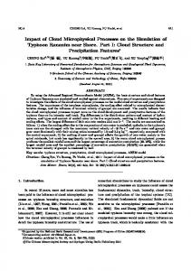
FIG. 12. Two-component number density distribution of droplets at different locations. From left to right: X 5 30, 60, and 90 km; from bottom to top: levels 1, 4, 7, and 10. The ordinates are the solute-mass bin number (left) or the corresponding dry radius (right), whereas the abscissas are the water-mass bin number (bottom) or the corresponding equivalent radius (top). The minimum contour is 10 26 per gram of air and increases by 100 times for each additional interval (values .1 g21 are highlighted). A 10-mM solute concentration isopleth is overlaid on each panel for reference. Also listed at the lower-right corner of each panel are the temperature, height, water saturation (Sw ), and ice saturation (Si ) of each layer.

of growth on the m w versus m s plot then switches to a direction parallel to the concentration isopleths. Thus, the diagonal orientation is a signature of riming. As mentioned in the previous sections, riming is an important mechanism for precipitation formation in the SN cloud, so such a signature exists in most of the panels in Fig. 13. The evidence of aggregation between pristine ice crystals can be seen at the lower part of panel B4 (Fig. 13). From the air temperature (214.28C) we realize that pristine ice crystals at this location may develop dendritic shapes that are optimal for mechanical interlocking when they collide. Because riming may take place on a portion of the aggregates, the distribution orien-

tation turns diagonally upward at reqv ; 100 mm. It is clear that these aggregates are much more diluted than are particles growing predominantly by riming. Once their reqv reach about 300 mm, riming becomes so efficient that the distribution immediately turns its orientation vertically upward and joins the cluster with the riming signature. Sufficient mass growth of the particles initiates the sedimentation process, which is evident in Fig. 13. For instance, the distribution of ice crystals in panel A2 resembles those with reqv . 100 mm in panel A3, indicating that they had fallen from aloft. In panels B1, B2, and B3, there exist some large but relatively dilute ice particles (the overhanging pattern at water bin 30) that were not present at earlier times. In addition,

2308

JOURNAL OF THE ATMOSPHERIC SCIENCES

VOLUME 56

FIG. 13. Same as Fig. 12 but for ice crystals. The bottom left panel shows the concentration isopleths (in mM) in logarithmic intervals, and the thick line highlights the 10-mM isopleth overlaid on all other panels.

these three panels do not exhibit the aggregation signature that appeared in panel B4, indicating that they are not produced locally but rather had fallen from the upper levels (see panel B4). Panel C4 of Fig. 13 is void of small ice crystals (reqv less than about 30 mm) that are common in other incloud (ice saturation $1) levels. Due to the descending air motion, the saturation ratio with respect to ice at this level has decreased to just above unity, prohibiting the production of ice crystals by deposition/condensationfreezing nucleation. Rime splintering, on the other hand, is not active either because of the unfavorable air temperature. Contact nucleation is also not possible since all cloud drops have evaporated. Yet the existing ice particles can nevertheless grow by aggregation and vapor diffusion, causing the number distribution in Fig. 13, panel C4, to differ from those in other panels.

c. Ice-phase particle framework—mw versus f The growth processes also left some footprints on the m w versus f diagrams shown in Fig. 14. Because all ice crystals are assumed to be symmetrical when they were first formed, the smallest ones started with an aspect ratio of unity. However, as is evident from the spreading of the distribution, these ice particles do not stay symmetrical as they grow. In fact, the most distinctive feature in many of the panels of Fig. 14 is the diagonally extended outer boundary of the particle distribution. Due to the habit development during diffusional growth, there is a tendency for small ice crystals to become more asymmetrical as they grow (cf. Chen and Lamb 1994a), a phenomenon best exemplified by the shaded area at reqv , 100 mm in panel B4. Such a signature is not as clear in other panels because of in-

15 JULY 1999

CHEN AND LAMB

2309

FIG. 14. Same as Fig. 13 but the ordinates are the shape bin number (left) or the corresponding aspect ratio (right). Bottom-left panel (A1) shows the divide between planar and columnar shapes at an aspect ratio of unity.

fluence from the riming and sedimentation processes. The association of growth habits with ambient temperature can be seen by comparing panels B2 (plates; 23.18C), B3 (columns; 28.08C), and B4 (plates; 214.28C). One may also notice the adaptation of growth habit to the change of ambient temperature. For example, the newly formed (reqv , 100 mm) ice crystals are plates in panel B2 but become columns in panel C2 (columns; 26.38C). A similar but opposite contrast can be seen between panels B3 and C3 (plates; 29.88C). In some panels (such as panels B2 and C1) one may notice that the larger (reqv . 100 mm) ice crystals tend to have growth habits opposite to those of the smaller crystals. One of the causes is that the larger ice crystals formed in a different habit regime. Then, when the air temperature switched to that of another habit regime, these ice crystals had already become too large and too asymmetrical to allow drastic habit change. The phe-

nomenon may also be caused by sedimentation. Take panel C4 for example, the air parcel was in the coldplate regime throughout the duration of cloud formation and yet contained a significant concentration of columnar crystals. These columns originated from the upper part of the cloud (see Fig. 5b). In panel B4 the diagonally oriented pattern (signature of diffusional growth) mentioned earlier makes a sudden change in direction at reqv ; 100 mm and created a ‘‘V-shaped’’ pattern. The inflection of cluster orientation at reqv ; 100 mm denotes a switch of the dominant growth mechanism from vapor diffusion to aggregation or riming, which tends to reduce the asymmetry of ice particles. Ice particles at levels below the cloud base (panels A2 and B1) have mixed shapes, with aspect ratios ranging from ;0.01 to ;100. However, the majority of these precipitation particles do not have extreme aspect ratios, indicating that they are mostly grau-

2310

JOURNAL OF THE ATMOSPHERIC SCIENCES

TABLE 5. Ratios of total mass and number produced in the SN cloud between different simulations. Whitby’s continental aerosol vs Jaenicke’s continental aerosol, C2/C1; Jaenicke’s maritime aerosol vs Jaenicke’s continental aerosol, M/C1. Number

All drops Cloud drop Raindrop All ice crystals Cloud ice Planar ice Columnar ice Rime ice Aggregate All condensates

Mass

C2/C1

M/C1

C2/C1

M/C1

0.357 0.355 2.301 0.807 0.728 0.830 1.044 0.764 0.385 0.381

0.202 0.175 37.243 0.484 0.349 0.424 0.586 0.937 0.225 0.217

0.804 0.793 1.590 0.814 0.646 2.279 0.995 0.551 0.767 0.808

0.632 0.613 2.007 0.798 0.308 2.069 1.037 0.936 0.098 0.709

pel or crystal aggregates. This result is consistent with the surface precipitation types shown in Fig. 9. 6. Sensitivity tests on AP size distribution The size distribution of aerosol particles has large spatial and temporal variations. In the simulation presented above, we applied the ‘‘remote continental’’ aerosol size distribution given by Jaenicke (1993). Due to a lack of observational data, it is unclear whether this distribution is suitable for the Sierra Nevada region in the particular season. One can alternatively apply the ‘‘clean continental background’’ aerosol distribution given by Whitby (1978), which by definition should represent a similar geographical area. Yet one can see from Table 2 that these two continental aerosol distributions are actually rather different. In order to understand the sensitivity of the model results to the assumed aerosol size distribution, two additional tests were performed, with one using Whitby’s clean continental background aerosol (case C2) and the other using Jaenicke’s ‘‘maritime’’ aerosol (case M) as model input. The original simulation will now be called ‘‘case C1.’’ To avoid tedious details, the following discussions will focus on microphysical properties integrated over the whole SN cloud. Table 5 shows the ratios of total number and mass of various cloud particles produced in case C2 and case M to those produced in case C1. One may first notice much lower CDN and somewhat lower LWC are developed in case C2 than in case C1. The reduction is even stronger for case M. The lower CDN is a direct response to the lower number concentration of APs (see Table 2), whereas the lower LWC is a result of less condensation (less total surface area) and more transformation into ice by riming. By contrast, the number concentration and water content of raindrops become significantly higher in case C2 and, especially, in case M. More detailed examination of the spatial distribution (not shown) would reveal that only 12% (1%) of the total number (mass) of raindrops exist within the cloud

VOLUME 56

TABLE 6. Same at Table 5 except for ice number generation. Number generation Overall generation Deposition/condensation-freezing nucleation Heterogeneous freezing Contact nucleation Rime splintering Aggregation

C2/C1

M/C1

0.707 1.029 0.772 0.393 0.977 0.170

0.431 2.962 0.688 0.150 0.310 0.162

in case C2, similar to the 15% (4%) in case C1. However, the situation is rather different for case M, where many of the raindrops (92% number and 41% mass) exist within the cloud. Since the base of the SN cloud is just above the 08C level, raindrops inside the cloud could not form by melting, rather by collision–coalescence (the situation in case M). On the other hand, if no significant rainwater exists inside the cloud, then the raindrops below the cloud base must be from melted ice (situation in cases C1 and C2). Therefore, case C2 shows a stronger cold-rain development than case C1, whereas case M shows more significant warm-rain processes. Note that in case M there are more (also larger) coarse mode APs, a condition favorable to the collision– coalescence process. Yet, in case M, the average size of raindrops below the cloud is much larger than that inside the cloud, which means a large fraction of the below-cloud raindrops is still created through the coldrain processes. The microphysical changes result in accumulated rainfall increases of 27% in case C2 and 29% in case M (see Table 6). A change in the initial AP distributions can also cause variations in the ice-phase processes. From Table 5 one can see that the number (mass) of ice crystals has reduced by about 19% (19%) in case C2 and 52% (20%) in case M compared to case C1. The most significant mass reduction in case C2 is in the rimed crystals, but for case M it is in crystal aggregates. However, the total mass of planar crystals becomes more than doubled in both case C2 and case M, because fewer of them are transformed into rimed crystals or aggregates. The reduction of total ice mass is strongly related to the reduction in crystal number concentration. Because of the lower number concentrations (the reason for which will be discussed later), there is less total surface area for water vapor to transform into ice by diffusional growth. In addition, a lower vapor deposition rate leads to higher saturation ratios, so each of the ice crystals grows faster. Also, crystals formed by contact nucleation are larger in case C2 and case M because of the larger initial drop sizes. Therefore, ice crystals formed in case C2 and case M are on the average larger than those in case C1, and they are removed faster from the atmosphere because of their higher fall speeds. The effects of AP distribution on the ice production are summarized in Table 6. Except for deposition/condensation-freezing nucleation, all ice production mechanisms have become less effective in case C2 and, es-

15 JULY 1999

CHEN AND LAMB

TABLE 7. Same as Table 5 except for surface precipitation. Surface precipitation Overall Liquid phase Ice phase

C2/C1

M/C1

1.033 1.274 0.711

1.071 1.204 0.893

pecially, in case M. The enhancement of deposition/ condensation-freezing nucleation is a result of the higher saturation ratios, which in turn is a result of lower particle concentrations. Heterogeneous nucleation is reduced since there are fewer cloud drops to freeze. The decline of cloud drop number concentration also reduced the chance for ice nuclei to collide with droplets. Thus, the occurrence of contact nucleation declined by more than 60% in case C2 and 85% in case M. The decline in contact nucleation, which is the most important ice generation mechanism in case C1, caused a significant reduction of overall ICN, which in turn affected the rate of rime splintering. Therefore, the reduction of AP concentration (case C2 and case M) caused an increase of ICN at the upper levels where deposition/condensation-freezing nucleation dominates, but a decrease at the lower levels where contact nucleation and rime splintering are more important. The increase in ICN at the upper levels does not help much in supplying ice crystals to the lower levels because the ice crystals there are now smaller and have lower fall speeds. Due to the lower ICN, the occurrence of crystal aggregation also diminished significantly. Less frequent occurrence of riming and aggregation, however, does not necessarily result in a decrease in the amount of precipitation. From Table 5 one can see that the degree of reduction in mass is generally less than that in number concentration, which means that the average size of cloud particles tends to increase as the number concentration becomes less. Because many of the microphysical mechanisms (such as contact nucleation and riming) are size dependent, the decrease in number concentration tends to be offset by an increase in individual growth rates and fall speeds. Such an effect is stronger at the earlier stage of cloud formation when there are more large droplets and then becomes less effective as the large drops are gradually consumed. Thus, from Table 7 we can see an increase in total rainfall (produced mostly by melting during the earlier stage) and a decrease in total snowfall for both case C2 and case M. Compared to case C1, the overall effect is to increase the total surface precipitation by 3.3% in case C2 and 7.1% in case M.

2311

ious physical and chemical properties of the cloud particles. The particle properties considered here are the water mass and solute content for both liquid drops and ice particles, as well as an additional shape factor for ice crystals. To facilitate discussions, the property distributions are subcategorized. Thus, simulated liquid drops are classified into interstitial aerosol particles, cloud drops, and raindrops, whereas ice crystals are classified into small cloud ice, planar crystals, columnar crystals, heavily rimed crystals, and crystal aggregates. We selected a case of cloud formation over the Sierra Nevada to study the details of mixed-phase processes. Microphysical properties, such as the number concentrations, water contents, and crystal habits, of the simulated cloud compare fairly well with observations. The main model results are summarized as follows.

7. Summary and conclusions

1) Supercooled liquid water content of up to 0.43 g m23 and ice water content of up to 0.65 g m23 are produced in the main cloud, whereas the maximum number concentrations of cloud drops, raindrops, and ice crystals are about 290 cm23 , 1.6 L21 , and 20 L21 , respectively. 2) Contact nucleation accounts for more than half of the total ice production in the cloud. Rime splintering is also an important ice production mechanism, especially in the warmer mixed-phase region. Deposition/condensation-freezing nucleation is important only at the upper (colder) part of the cloud. 3) Precipitation development occurs primarily through the cold-cloud processes: rainfall is formed mainly through the melting of snow, whereas snowfall is formed mainly through riming and aggregation. 4) About 17% of the water vapor entering the cloud can be removed from the air as precipitation. The large size of the orographic cloud is a significant factor contributing to a high precipitation efficiency. 5) Most of the ice crystals contain significant amounts of solute, especially those with equivalent radii, exceed a few hundred microns, a result of significant riming. 6) The shapes of vapor-grown crystals clearly reflect habit development in accordance with the ambient temperatures. However, sedimentation or a change of air temperature during crystal growth may cause the mixture of crystal types that result. While vaporgrown crystals become more asymmetric as they become bigger, riming and aggregation tend to reduce the asymmetry. 7) Examination of the shape and solute concentration of individual ice particles provides useful information about their birth and growth history.

This study applied a microphysical model to simulate the formation of a wintertime orographic cloud in a twodimensional domain using a steady-state approach. By utilizing a multicomponent particle framework, this model is able to describe simultaneous changes of var-

To test the effects of AP size distribution on the formation of cloud and precipitation, additional simulations were done using different types of aerosol distribution as initial model input. The main findings from these sensitivity tests are summarized below.

2312

JOURNAL OF THE ATMOSPHERIC SCIENCES

1) The size distribution of APs has significant influence on not only the warm-cloud processes but also the cold-cloud processes. 2) A lower AP concentration generally produces fewer but larger cloud drops, which in turn results in higher saturation ratios in the cloud and enhanced production of ice by deposition/condensation-freezing nucleation, but reduced occurrence of contact nucleation. The production of ice crystals by rime splintering also decreases because of the lower cloud drop and ice crystal number concentrations. 3) Growth of individual ice crystals, on the other hand, can be enhanced when there are sufficient large drops and higher saturation ratios. 4) The net effect of lower number concentrations and higher individual growth rates is to enhance the development of precipitation during the earlier stage of cloud formation but depress it at the later stage. The overall precipitation amount is increased when the initial AP concentration is lower. This study has demonstrated the application of a multicomponent particle model in simulating the microphysical properties of an orographic cloud with great details. Such a model may be further applied in studying the effects of warm-cloud or cold-cloud seeding. The ability to resolve different forms of precipitation particles also enables the study of chemical removal processes in mixed-phase clouds, a topic that will be discussed in the sequel to this paper. Acknowledgments. We appreciate the cooperation of personnel associated with SCPP and the WMO, as well as of other participants of the Third International Modeling Workshop (1992) who provided data for model setup and valuable insights on this case. This research was supported in various parts by the National Science Council under Grant NSC-87-2111-M-002, the Department of Energy under Grant DE-FG02-90ER61071, and the National Science Foundation under Grants ATM8919837 and ATM-9319119. REFERENCES Braham, R. R., Jr., 1952: The water and energy budgets of the thunderstorm and their relation to thunderstorm development. J. Meteor., 9, 227–242. Chen, J.-P., 1994a: Predictions of saturation ratio for cloud microphysical models. J. Atmos. Sci., 51, 1331–1338. , 1994b: Theory of deliquescence and modified Ko¨hler curves. J. Atmos. Sci., 51, 3505–3516. , and D. Lamb, 1994a: The theoretical basis for the parameterization of ice crystal habits: Growth by vapor deposition. J. Atmos. Sci., 51, 1207–1221. , and , 1994b: Simulation of cloud microphysical and chemical processes using a multicomponent framework. Part I: Description of the microphysical model. J. Atmos. Sci., 51, 2613– 2630. Demoz, B. B., R. Zhang, and R. Pitter, 1993: An analysis of Sierra

VOLUME 56

Nevada winter orographic storms: Ground-based ice-crystal observation. J. Appl. Meteor., 32, 1826–1836. Deshler, T., and D. W. Reynolds, 1990: The persistence of seeding effects in a winter orographic cloud seeded with silver iodide burned in acetone. J. Appl. Meteor., 29, 477–488. , , and A. W. Huggins, 1990: Physical response of winter orographic clouds over the Sierra Nevada to airborne seeding using dry ice or silver iodide. J. Appl. Meteor., 29, 288–330. Elliott, R. D., and E. L. Hovind, 1964: The water balance of orographic clouds. J. Appl. Meteor., 3, 235–239. Hallett, J., and B. J. Mason, 1958: The influence of temperature and supersaturation on the habit of ice crystals grown from the vapor. Proc. Roy. Soc. London, 247A, 440–453. Hobbs, P. V., 1975: The nature of winter clouds and precipitation in the Cascade Mountains and their modification by artificial seeding. Part I: Natural conditions. J. Appl. Meteor., 14, 783–l803. , R. C. Easter, and A. B. Fraser, 1973: A theoretical study of the flow of air and fallout of solid precipitation over mountainous terrain: Part II. Microphysics. J. Atmos. Sci., 30, 813–823. Huffman, P. J., 1973: Supersaturation spectra of AgI and natural ice nuclei. J. Appl. Meteor., 12, 1080–1082. Huggins, A. W., R. J. Meitin, and R. F. Reinking, 1990: Comparison of radiometric measurements of cloud liquid water near a mountain crest and over a downwind valley. Preprints, Fifth Conf. on Mountain Meteorology, Boulder, CO, Amer. Meteor. Soc., 135–142. Jaenicke, R., 1993: Tropospheric aerosols. Aerosol–Cloud–Climate Interactions, P. V. Hobbs, Ed., Academic Press, 1–31. Kobayashi, T., 1961: The growth of snow crystals at low supersaturations. Philos. Mag., 6, 1363–1370. Meyers, M. P., P. J. DeMott, and W. R. Cotton, 1995: A comparison of seeded and nonseeded orographic cloud simulations with an explicit cloud model. J. Appl. Meteor., 34, 834–846. Mitchell, D. L., 1988: Evolution of snow-size spectra in cyclonic storms. Part I: Snow growth by vapor deposition and aggregation. J. Atmos. Sci., 45, 3431–3451. Mossop, S. C., 1976: Production of secondary ice particles during the growth of graupel by riming. Quart. J. Roy. Meteor. Soc., 102, 45–57. Myers, V. A., 1962: Airflow on the windward side of a ridge. J. Geophys. Res., 67, 4267–4291. Nakaya, U., 1954: Snow Crystals: Natural and Artificial. Harvard University Press, 510 pp. Ochs, H. T., III, and C. S. Yao, 1978: Moment-conserving techniques for warm cloud microphysical computations. Part II: Model testing and results. J. Atmos. Sci., 35, 1959–1973. Prasdad, N., A. R. Rodi, and A. J. Heymsfield, 1989: Observations and numerical simulations of precipitation development in seeded clouds over the Sierra Nevada. J. Appl. Meteor., 28, 1031–1049. Pruppacher, H. R., and J. D. Klett, 1997: Microphysics of Clouds and Precipitation. 2d ed., Kluwer Academic, 954 pp. Rauber, R. M., R. D. Elliott, J. O. Rhea, A. W. Huggins, and D. W. Reynolds, 1988: A diagnostic technique for targeting during airborne seeding experiments in wintertime storms over the Sierra Nevada. J. Appl. Meteor., 27, 811–828. Reynolds, D. W., and A. P. Kuciauskas, 1988: Remote and in situ observations of Sierra Nevada winter mountain clouds: Relationships between mesoscale structure, precipitation and liquid water. J. Appl. Meteor., 27, 140–156. Takahashi, T., T. Endoh, G. Wakahama, and N. Fukuta, 1991: Vapor diffusional growth of free-falling snow crystals between 23 and 2238C. J. Meteor. Soc. Japan, 69, 15–30. Twomey, S., 1959: The nuclei of natural cloud formation, Part II: The supersaturation in natural clouds and the variation of cloud droplet concentration. Geofys. Pura e Appl., 43, 243–249. Young, K. C., 1974: A numerical simulation of wintertime, orographic precipitation: Part II: Comparison of natural and AgI seeded conditions. J. Atmos. Sci., 31, 1749–1767. Whitby, K. T., 1978: The physical characteristics of sulfur aerosols. Atmos. Environ., 12, 135–159.