SIMULATION OF IMPROVED GAUSSIAN TIME ... - Google Sites

SIMULATION OF IMPROVED GAUSSIAN T I M E HISTORY By Loren D. Lutes,' Fellow, ASCE, and Jim Wang, 2 Student Member, ASCE INTRODUCTION

A conventional technique for simulating a Gaussian time history generates the Gaussian signal by summing up a number of sine waves with random phase angles and either deterministic or random amplitudes. After this simulated process has been used as the input to some system, unknown response expectations are generally estimated from time averages for stationary processes. However, the values of the expectation estimates based on single time histories may exhibit a considerable amount of scatter or statistical inaccuracy because of two facts: only a limited number of terms have been used in the frequency summation; and the time history is only of finite length. This statistical inaccuracy is usually not a serious problem for estimating mean and variance, but it may be a problem in estimating probabilities of failure, which often are more affected by the tails of the probability distribution. Presented herein is an approach from which an improved Gaussian time history can be obtained, in which the time-average moments are exactly equal to the corresponding theoretical expectations for a Gaussian process. It is shown that the joint moments and the moments of extrema of the improved time history also agree with the corresponding properties for the Gaussian process, providing stronger evidence for considering the time history as a representative sample from a Gaussian process.

PROBLEM FORMULATION

A standard procedure, commonly referred to as the Gaussian technique, for simulating a Gaussian time history generates the random Gaussian signal from a one-sided power spectral density (PSD) Gx(co), according to the equation N

X{t) = 2

V2Gx(a>,)Aw, sin (u(f + 6 , )

(1)

in which Aw, = the frequency interval; to, = the midpoint of the frequency interval; and 0, = the random phase angle, uniform on [0,2ir]. Time-average expectation estimates are calculated by EQC) = I,j=lX]'/N, where X, = X(tj). It is not uncommon that the time-average moments evaluated from time 'Prof, of Civ. Engrg., Texas A&M Univ., College Station, TX 77843-3136. 2 Grad. Res. Asst., Texas A&M Univ., College Station, TX. Note. Discussion open until June 1, 1991. To extend the closing date one month, a written request must be filed with the ASCE Manager of Journals. The manuscript for this paper was submitted for review and possible publication on February 2, 1990. This paper is part of the Journal of Engineering Mechanics, Vol. 117, No. 1, January, 1991. ©ASCE, ISSN 0733-9399/91/0001-0218/$1.00 + $.15 per page. Paper No. 25407. 218 Downloaded 18 Jun 2010 to 129.15.14.53. Redistribution subject to ASCE license or copyright. Visit

http://w

histories simulated using the conventional Gaussian technique show considerable variations, and the variations grow as m grows. In engineering applications, it is often necessary to look at moments higher than the variance. For example, fatigue damage generally varies like some measure of stress to a power m. For welded connections or points of high stress concentration, m is usually about 3 or 4 (Lutes et al. 1984). However, if the stress is a nonlinear function, say a cubic function, of a Gaussian process X, then the fatigue damage may involve moments of X as high as 9 or 12. Improved simulation might be done by replacing the deterministic amplitude terms in Eq. 1 with independent Rayleigh variables with the same mean-square value, or by increasing the number of terms of the cosine functions in the summation, or by using more sophisticated techniques (Yamazaki and Shinozuka 1990). More commonly, a long simulated time history or an ensemble of time histories is used to get stable moment estimates in simulation studies. In this situation, the procedure of numerically simulating the response of a complicated nonlinear system will become increasingly time consuming even though the simulation of the Gaussian time history itself may be done very efficiently by an FFT procedure. The technique presented here to obtain a sequence having exact Gaussian moments is to use a nonlinear transformation of a weakly non-Gaussian sequence. This is the inverse of a commonly used technique for generating a non-Gaussian process by a nonlinear transformation of a Gaussian process. In particular, the initial nearly Gaussian time history is simulated using Eq. 1. The question then is whether it is possible to modify this nearly Gaussian time history by a nonlinear transformation to obtain a single representative time history whose time-average moments agree with the expectations for a Gaussian process, even though the time history is of limited length. FITTING TIME-AVERAGE MOMENTS

A stationary Gaussian process {X(t)} with zero mean has the moment property E{Xm) = 1 • 3 • 5 . . . (m -

1)CT™,

for m = 2, 4, 6,

(2)

in which . Then X(t) may be obtained by a transformation function of Y(t), i.e. X(t) = g[Y(t)]

(3)

where g(*) = a nonlinear monotonic function. This nonlinear transformation can be approximated by a polynomial expansion as in

X{t) = 2 P„£/"(0

(4)

in which U(t) = [Y(t) — ftyl/oy with zero mean and unit standard deviation. To relate the unknown coefficients in Eq. 4 to the time-average moments 219 Downloaded 18 Jun 2010 to 129.15.14.53. Redistribution subject to ASCE license or copyright. Visit

http://ww

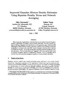
GENERATE TIME SEQUENCE: (Y„ Y2, • •.Y • N)

+ OBTAIN INITIAL X SEQUENCE:

X, = Y i

FIND MEAN AND VARIANCE: nK = — f,Xj

al = —

I,(.Xrfix)-

I OBTAIN STANDARDIZED SEQUENCE: (U„U 2 ,- •.u N }

EVALUATE MOMENTS:

{AJ 3 ,/J 4 ,-,/l m „}

IE

I C H E C K FOR C O N V E R G E N C E OF

NO

EVALUATE HERMITE COEFFICIENTS:

_Xr/ix U

-"k = ^ |

i

U

?

(/J3,^4,---,/i„

YES (h 3 ,h 4 ,---,h m+1 )

* STOP

hk = - - I H e , ( ( U i )

IE MODIFY THE X SEQUENCE:

X, = U, - X h ^ H e ^ U p

T FIG. 1.

Flowchart for Transformation and Iteration

of U(t), Eq. 4 can be rearranged into a Hermite series (Winterstein 1988) as follows X = U - 2 hn+lHen(U)

(5)

in which * , » = (-!)« exp -

- exp

n = 0, 1, 2,

(6)

For example, //