An Improved Gaussian Mixture CKF Algorithm under Non-Gaussian ...

Hindawi Publishing Corporation Discrete Dynamics in Nature and Society Volume 2016, Article ID 1082837, 10 pages http://dx.doi.org/10.1155/2016/1082837

Research Article An Improved Gaussian Mixture CKF Algorithm under Non-Gaussian Observation Noise Hongjian Wang and Cun Li College of Automation, Harbin Engineering University, Harbin 150001, China Correspondence should be addressed to Cun Li; [email protected] Received 14 March 2016; Revised 10 June 2016; Accepted 16 June 2016 Academic Editor: Juan R. Torregrosa Copyright © 2016 H. Wang and C. Li. This is an open access article distributed under the Creative Commons Attribution License, which permits unrestricted use, distribution, and reproduction in any medium, provided the original work is properly cited. In order to solve the problems that the weight of Gaussian components of Gaussian mixture filter remains constant during the time update stage, an improved Gaussian Mixture Cubature Kalman Filter (IGMCKF) algorithm is designed by combining a Gaussian mixture density model with a CKF for target tracking. The algorithm adopts Gaussian mixture density function to approximately estimate the observation noise. The observation models based on Mini RadaScan for target tracking on offing are introduced, and the observation noise is modelled as glint noise. The Gaussian components are predicted and updated using CKF. A cost function is designed by integral square difference to update the weight of Gaussian components on the time update stage. Based on comparison experiments of constant angular velocity model and maneuver model with different algorithms, the proposed algorithm has the advantages of fast tracking response and high estimation precision, and the computation time should satisfy real-time target tracking requirements.

1. Introduction With the universality of nonlinear problems, the principle and method of nonlinear filtering are being widely used for the nonlinear systems. One of the applications is target states estimation. For the currently nonlinear systems, the possible solution approaches are some approximate methods, such as approximating the probability density of system state as the Gaussian density, which is called Gaussian filtering. The Gaussian filtering could sum up three classes according to the different approximate methods: the first is function approximation, which approximates the nonlinear system function using the low-order expansion such as the extended Kalman filtering (EKF) [1] and the improved algorithms (adaptive fading EKF [2], strong tracking EKF [3], and central difference Kalman filtering (CDKF) [4, 5]). The EKF is a suboptimal filter that demands not only that the system has accurate states and accurate observation models but also that the observation noise is Gaussian in nature. However, the Gaussian Hypothesis is poor when the system model is highly nonlinear, and the estimation results are divergent. The CDKF based on Stirling’s polynomial interpolation has better performance including

accuracy, efficiency, and stability than EKF for the nonlinear problems but would cause the greater computation burden. The second is deterministic sampling approximation method, which approximates system state and the probability density using deterministic sampling such as the Unscented Kalman Filter (UKF) [6, 7] and the improved algorithms [8, 9]. In principle, the UKF is simple and easy to implement, as it does not require the calculation of Jacobians at each time step. However, the UKF requires updating the matrix with sigma points with weighted negative values, which makes it difficult to preserve the positive definiteness during the iterative filter process. The third is approximation using quadrature, which approximates the multidimensional integrals of Bayesian recursive equation using some numerical technologies, such as the Gaussian-Hermite Kalman Filter (GHKF) [10] and the Cubature Kalman Filter (CKF) [11–13]. GHKF acquires the statistic characteristics after nonlinear transformation by Gaussian-Hermite numerical integral, which has higher accuracy. The shortcoming of GHKF is that it may not be suitable for addressing the high-dimensional nonlinear filtering issue. The CKF is proposed based on the sphericalradial cubature rule and can solve the Bayesian filter integral problem using cubature points with the same weight. The

2

Discrete Dynamics in Nature and Society

high-degree CKFs have high accuracy and stability but at a high computational cost. In actual application on target tracking, the noise of system processes or observations do not have ideal Gaussian density. In addition, the various Gaussian approximate filtering algorithms based on Gaussian noise do not display ideal performance because of the mismatched model. Besides Gaussian filter, other solution approaches for the nonlinear estimation problem involve the particle filter (PF) [14] based on the Monte Carlo numerical integral theory and sequence importance sampling and Gaussian sum filter [15, 16] based on the mixture of several Gaussian components. Although the PF do not require any assumption about the probability density function, they inevitably face enormous undesirable computational demands owing to the numerous stochastic sampling particles for fulfilling the estimation accuracy. The PF algorithm is unable to avoid the disadvantages of particle degradation and sample dilution; hence, the research on PF is focused on the revolution of particle degradation and sample dilution [17, 18]. A Gaussian sum CKF has been proposed for bearings-only tracking problems in the literature [19], and this CKF displays comparable performance to the particle filter. An improved Gaussian mixture filter algorithm has been proposed for highly nonlinear passive tracking systems in the literature [20], and the limited Gaussian mixture model has been used to approximate the posterior density of the state, process noise, and measurement noise. However, in all of these methods, the weights of the Gaussian components are kept constant while propagating the uncertainty through a nonlinear system and are updated only in the stage of measurement update. This assumption is valid if the system is marginally nonlinear or measurements are precise and available very frequently. The same is not true for the general nonlinear case. Terejanu et al. [21, 22] proposed a new Gaussian sum filter by adapting the weights of Gaussian mixture model in case of both time update and measurement update, which could obtain a better approximation of the posterior probability density function. In this paper, we focus on the target tracking problem on offing and design an improved Gaussian mixture CKF based on the GMCKF algorithm. Firstly, the formulation of target tracking is described, and the observation model with glint noise based on sensor is introduced. Secondly, the derivate steps of IGMCKF based integral square difference and Gaussian mixture density are designed. At last, the comparison experiments of constant angular velocity model and maneuver model with different algorithms are present, respectively.

2. Problem Formulation Consider the target tracking problem on offing, giving the motion model and observation model: x𝑘 = 𝐹x𝑘−1 + w𝑘−1 , z𝑘 = ℎ (x𝑘 ) + k𝑘 , 𝑇

(1)

where x𝑘 = [𝑥, 𝑥,̇ 𝑦, 𝑦]̇ (𝑘) denotes the target states, including the position and velocity of the target, and w𝑘−1 denotes

the state process noise, which is assumed as Gaussian density with covariance 𝑄. k𝑘 denotes the observation noise which is assumed as glint noise because of the complicated environment on offing and the characteristics of sensors. The observation noise could be approximated as glint noise which is composed of Gaussian noise and Laplace noise. We modelled the observation noise as 2 Gaussian components with different covariance: 𝑝 (V) = (1 − 𝜀) 𝑁 (V; 𝑢1 , 𝑅1 ) + 𝜀𝑁 (V; 𝑢2 , 𝑅2 ) ,

(2)

where 𝑁(V; 𝑢, 𝑅) denotes Gaussian noise with mean 𝑢 and covariance 𝑅. 𝜀 ∈ [0, 1] is the glint frequency factor. Consider that the position of sensor is (𝑥0 , 𝑦0 ), and the sensor in this paper is Mini RadaScan; the observation information of the target including distance and bearing is as follows: 2 2 √ [ (𝑥𝑘 − 𝑥𝑜 ) + (𝑦𝑘 − 𝑦𝑜 ) ] ]. ℎ (x𝑘 ) = [ ] [ 𝑦 − 𝑦𝑜 arctan ( 𝑘 ) 𝑥𝑘 − 𝑥𝑜 ] [

(3)

3. Design of Improved Gaussian Mixture Cubature Kalman Filter Algorithm Lemma 1. The probability density function of the 𝑛-dimension vector 𝑥 can be approximated by the following equation: 𝐼

𝑝 (𝑥) = ∑𝜔𝑖 𝑁 (𝑥; 𝜇𝑖 , 𝑃𝑖 ) .

(4)

𝑖=1

The approximate error can be arbitrarily small as soon as the number of components 𝐼 is large enough. 𝜔𝑖 denotes the weighted value of the 𝑖th component; 𝑁(𝑥; 𝜇𝑖 , 𝑃𝑖 ) denotes the Gaussian distribution with mean 𝜇𝑖 and covariance 𝑃𝑖 . Consider 𝐼

∑𝜔𝑖 = 1, 𝑖=1

𝑁 (𝑥; 𝜇𝑖 , 𝑃𝑖 ) =

1

√2𝜋 󵄨󵄨󵄨󵄨𝑃𝑖 󵄨󵄨󵄨󵄨

(5) 1 𝑇 −1 exp (− (𝑥 − 𝜇𝑖 ) (𝑃𝑖 ) (𝑥 − 𝜇𝑖 )) . 2

3.1. Time Update. Consider that the discrete nonlinear system with Gaussian mixture added noise and the prior and posterior density can be indicated by a Gaussian sum. The process noise and observation noise could be approximated as follows: 𝐽

𝑝

𝑝 (𝑤𝑘 ) ≈ ∑𝜔𝑘 (𝑗) 𝑁 (𝑤𝑘 ; 𝑤𝑘 , 𝑄𝑘 (𝑗)) , 𝑗=1

𝑝 (V𝑘 ) ≈

𝐿

∑𝜔𝑘𝑚 𝑙=1

(6) (𝑙) 𝑁 (V𝑘 ; V𝑘 , 𝑅𝑘 (𝑙)) ,

Discrete Dynamics in Nature and Society

3

where 𝛼𝑘 (𝑗) denotes the weighted value of the 𝑗th component of the process noise and 𝛽𝑘 (𝑙) is the weighted value of the 𝑙th component of the observation noise. Consider 𝐽

𝑝

∑𝜔𝑘 (𝑗) = 1,

𝑗=1

(7)

𝐿

𝐼

∑𝜔𝑘𝑚 (𝑙) = 1.

̂ (x𝑘 ) = ∑𝜔𝑘𝑠 (𝑖) 𝑁 (x𝑘 (𝑖) ; x̂𝑘 (𝑖) , 𝑃𝑘 (𝑖)) . 𝑝

𝑙=1

𝐼

𝑖=1

We can obtain the prior density of state transition equation by the following equation: 𝑝 (x𝑘 | x𝑘−1 ) 𝑝

= ∑𝜔𝑘−1 (𝑗) 𝑁 (x𝑘 ; 𝑓 (x𝑘−1 ) + 𝑤𝑘 (𝑗) , 𝑄𝑘 (𝑗)) .

(9)

𝑗=1

According to the Bayesian formula, the predicted state density function can be approximated using a Gaussian mixture model: 𝑝 (x𝑘 | z1:𝑘−1 ) 𝐼

𝑝

𝑠 = ∑ ∑𝜔𝑘−1 (𝑖) 𝜔𝑘 (𝑗) ∫

𝑅𝑛𝑥

𝑗=1 𝑖=1

𝑝 (x𝑘 ) = ∫ 𝑝 (x𝑘 | x𝑘−1 ) 𝑝 (x𝑘−1 ) 𝑑x𝑘−1 .

(13)

R𝑛

Mean-square optimal new weights can be obtained by minimizing the following integral square difference between ̂ (x𝑘 ) the true probability 𝑝(x𝑘 ) and the approximation one 𝑝 in the least square algorithm:

w𝑘|𝑘−1 = arg min

1 ̂ (x𝑘 ))2 𝑑x𝑘 , ∫ (𝑝 (x𝑘 ) − 𝑝 2 R𝑛

(14)

𝑇

𝑁 (x𝑘−1 ; x̂𝑘−1 (𝑖) , 𝑃𝑘−1 (𝑖))

⋅ 𝑁 (x𝑘 ; 𝑓 (x𝑘−1 ) + 𝑤 (𝑗) , 𝑄𝑘 (𝑗)) 𝑑x𝑘−1 𝐽

The true probability density function of system state by the Chapman-Kolmogorov equation is given:

(8)

𝑠 = ∑𝜔𝑘−1 (𝑖) 𝑁 (x𝑘−1 ; x̂𝑘−1 (𝑖) , 𝑃𝑘−1 (𝑖)) .

𝐽

(12)

𝑖=1

Then, consider that the posterior density can be approximated with a Gaussian mixture model at 𝑘 − 1: 𝑝 (x𝑘−1 | z1:𝑘−1 )

𝐽

3.2. Adaptive Weight Update. Consider the following nonlinear system (1) with the probability density function of the initial conditions 𝑝(𝑥0 ). According to formula (4), the Gaussian mixture approximation of the probability density function is given:

(10)

where w𝑘|𝑘−1 = [𝜔𝑘|𝑘−1 (1) 𝜔𝑘|𝑘−1 (2) ⋅ ⋅ ⋅ 𝜔𝑘|𝑘−1 (𝐼)] denotes the vector of the weights of every Gaussian component at time 𝑘. In order to resolve formula (17), the cost function is given as follows [23]:

𝐼

≈ ∑ ∑𝜔𝑘|𝑘−1 (𝑖, 𝑗) 𝑁 (x𝑘 ; x̂𝑘|𝑘−1 (𝑖, 𝑗) , 𝑃𝑘|𝑘−1 (𝑖, 𝑗))

̂

𝐽 (w𝑘|𝑘−1 ) = 𝐽𝑝𝑝 (w𝑘|𝑘−1 ) − 2𝐽𝑝𝑝 (w𝑘|𝑘−1 )

𝑗=1 𝑖=1

̂̂

+ 𝐽𝑝𝑝 (w𝑘|𝑘−1 ) ,

𝐼⋅𝐽

𝑡 ≈ ∑𝜔𝑘|𝑘−1 (𝑟) 𝑁 (x𝑘 ; x̂𝑘|𝑘−1 (𝑟) , 𝑃𝑘|𝑘−1 (𝑟)) ,

(15)

𝑟=1

𝑝

𝑡 𝑠 where 𝜔𝑘|𝑘−1 (𝑟) = 𝜔𝑘−1 (𝑖)𝜔𝑘 (𝑗). 𝑅 is the set of real numbers, and 𝑛𝑥 is the dimension of the state vector. 𝐼 and 𝐽 are the number of Gaussian components of system state and process noise, respectively. x̂𝑘|𝑘−1 (𝑟) and 𝑃𝑘|𝑘−1 (𝑟) could be calculated by the time update steps of CKF: 𝑚

x̂𝑘|𝑘−1 (𝑟) = ∑𝜔𝑐 𝜉𝑐,𝑘|𝑘−1 (𝑖) + 𝑤𝑘 (𝑗) , 𝑐=1

𝑃𝑘|𝑘−1 (𝑟) 𝑚

(11)

𝑇 = ∑𝜔𝑐 𝜉𝑐,𝑘|𝑘−1 (𝑖) 𝜉𝑐,𝑘|𝑘−1 (𝑖) 𝑐=1

𝑇

− [̂x𝑘|𝑘−1 (𝑟) − 𝑤𝑘 (𝑗)] [̂x𝑘|𝑘−1 (𝑟) − 𝑤𝑘 (𝑗)] + 𝑄𝑘 (𝑗) , where 𝑚 is the number of cubature points.

where the first term represents the self-likeness of the true probability density function of the system state and 𝐽𝑝𝑝 (w𝑘|𝑘−1 ) = ∫R𝑛 𝑝(x𝑘 )𝑝(x𝑘 )𝑑x𝑘 . The first term is not needed in the optimization process and it is used only to provide an overall magnitude of the uncertainty propagation error [24]. The second represents the cross-likeness of the true probability and the approximation one, and ̂ (x𝑘 )𝑑x𝑘 . The last term is the self𝐽𝑝𝑝̂ (w𝑘|𝑘−1 ) = ∫R𝑛 𝑝(x𝑘 )𝑝 likeness of the approximation probability of the system state, ̂ (x𝑘 )𝑝 ̂ (x𝑘 )𝑑x𝑘 . and 𝐽𝑝̂ 𝑝̂ (w𝑘|𝑘−1 ) = ∫R𝑛 𝑝 Formula (16) is based on the assumption that the Gaussian mixture approximation is equal to the true probability ̂ (x𝑘−1 ) = 𝑝(x𝑘−1 ). density function at time 𝑘 − 1; namely, 𝑝 Consider ̂ (x𝑘−1 ) 𝑑x𝑘−1 . 𝑝 (x𝑘 ) = ∫ 𝑝 (x𝑘 | x𝑘−1 ) 𝑝 R𝑛

(16)

4

Discrete Dynamics in Nature and Society 𝐼

Now the derivation of the terms of cost function is given as follows:

𝑠 = ∫ [∫ 𝑁 (x𝑘 ; 𝑓 (x𝑘−1 ) + 𝑤𝑘 , 𝑄𝑘 ) = ∑𝜔𝑘−1 (𝑖) R𝑛

R𝑛

𝑖=1

2

2

𝐽𝑝𝑝 (w𝑘|𝑘−1 ) = ∫ 𝑝 (x𝑘 ) 𝑑x𝑘 = ∫ [∫ 𝑝 (x𝑘 | x𝑘−1 ) R𝑛

R𝑛

⋅ 𝑁 (x𝑘−1 (𝑖) ; x̂𝑘−1 (𝑖) , 𝑃𝑘−1 (𝑖)) 𝑑x𝑘−1 ] 𝑑x𝑘

R𝑛

2

𝑇 = w𝑘−1 𝐽𝑝𝑝 w𝑘−1 .

⋅ 𝑝 (x𝑘−1 ) 𝑑x𝑘−1 ] 𝑑x𝑘

(17)

2

̂ (x𝑘−1 ) 𝑑x𝑘−1 ] 𝑑x𝑘 = ∫ [∫ 𝑝 (x𝑘 | x𝑘−1 ) 𝑝 R𝑛

Similarly,

R𝑛

R𝑛

̂

̂

̂̂

̂̂

𝑇 𝐽𝑝𝑝 (w𝑘|𝑘−1 ) = w𝑘|𝑘−1 𝐽𝑝𝑝 w𝑘−1 ,

= ∫ [∫ 𝑁 (x𝑘 ; 𝑓 (x𝑘−1 ) + 𝑤𝑘 , 𝑄𝑘 ) R𝑛

(18)

𝑇 𝐽𝑝𝑝 w𝑘|𝑘−1 . 𝐽𝑝𝑝 (w𝑘|𝑘−1 ) = w𝑘|𝑘−1

2

̂ (x𝑘−1 ) 𝑑x𝑘−1 ] 𝑑x𝑘 ⋅𝑝

The elements of the matrix are given as follows: 2

𝑝𝑝

𝐽𝑖𝑗 = ∫ [∫ 𝑁 (x𝑘 ; 𝑓 (x𝑘−1 ) + 𝑤𝑘 , 𝑄𝑘 ) 𝑁 (x𝑘−1 (𝑖) ; x̂𝑘−1 (𝑖) , 𝑃𝑘−1 (𝑖)) 𝑑x𝑘−1 ] 𝑑x𝑘 2

= ∫ (𝐸𝑁(x𝑘−1 (𝑖);̂x𝑘−1 (𝑖),𝑃𝑘−1 (𝑖)) [𝑁 (x𝑘 ; 𝑓 (x𝑘−1 ) + 𝑤𝑘 , 𝑄𝑘 )]) 𝑑x𝑘 , (19)

̂ 𝑝𝑝

𝐽𝑖𝑗 = ∫ 𝑁 (𝑓 (x𝑘−1 ) ; x𝑘|𝑘−1 (𝑖) , 𝑃𝑘|𝑘−1 (𝑖) + 𝑄𝑘−1 ) 𝑁 (x𝑘−1 ; x𝑘−1 (𝑗) , 𝑃𝑘−1 (𝑗)) 𝑑x𝑘−1 = 𝐸𝑁(x𝑘−1 ;x𝑘−1 (𝑗),𝑃𝑘−1 (𝑗)) [𝑁 (𝑓 (x𝑘−1 ) ; 𝑚

x𝑘|𝑘−1 (𝑖) , 𝑃𝑘|𝑘−1 (𝑖) + 𝑄𝑘−1 )] = ∑𝜔𝑐 𝑁 (𝜉𝑐,𝑘|𝑘−1 ; x𝑘|𝑘−1 (𝑖) , 𝑃𝑘|𝑘−1 (𝑖)) , 𝑐=1

where (𝜔𝑐 , 𝜉𝑐 ) is the cubature points. Consider

Then, we can obtain the following equation: 𝐿 𝐼⋅𝐽

̂𝑝 ̂ 𝑝

𝑡 𝑝 (x𝑘 | z1:𝑘 ) = ∑ ∑𝜔𝑘𝑚(𝑙) 𝜔𝑘|𝑘−1 (𝑟)

𝐽𝑖𝑗 = 𝑁 (x𝑘|𝑘−1 (𝑖) ; x𝑘|𝑘−1 (𝑗) , 𝑃𝑘|𝑘−1 (𝑖) + 𝑃𝑘|𝑘−1 (𝑗))

𝑙=1 𝑟=1

󵄨−1/2 󵄨 = 󵄨󵄨󵄨2𝜋 (𝑃𝑘|𝑘−1 (𝑖) + 𝑃𝑘|𝑘−1 (𝑖))󵄨󵄨󵄨 1 𝑇 ⋅ exp [− (x𝑘|𝑘−1 (𝑖) − x𝑘|𝑘−1 (𝑗)) 2

(20)

⋅∫

𝑅𝑛𝑥

𝑁 (x𝑘 ; x̂𝑘|𝑘−1 (𝑟) , 𝑃𝑘|𝑘−1 (𝑟))

⋅ 𝑁 (z𝑘 ; ℎ (x𝑘 ) + V𝑘 (𝑙) , 𝑅𝑘 (𝑙)) 𝑑x𝑘

(23)

𝐿 𝐼⋅𝐽

𝑡 = ∑ ∑𝜔𝑘𝑚 (𝑙) 𝜔𝑘|𝑘−1 (𝑟) 𝑁 (x𝑘 ; x̂𝑘 (𝑟, 𝑙) , 𝑃𝑘 (𝑟, 𝑙))

−1

⋅ (𝑃𝑘|𝑘−1 (𝑖) + 𝑃𝑘|𝑘−1 (𝑖)) (x𝑘|𝑘−1 (𝑖) − x𝑘|𝑘−1 (𝑗))] .

𝑝=1 𝑟=1

According to the above relations, the final formulation of formula (14) could be obtained as follows: 1 𝑇 ̂ ̂̂ 𝑇 𝐽𝑝𝑝 w𝑘|𝑘−1 − w𝑘|𝑘−1 𝐽𝑝𝑝 w𝑘−1 ; (21) w𝑘|𝑘−1 = arg min w𝑘|𝑘−1 2

𝐼⋅𝐽⋅𝐿

= ∑ 𝜔𝑘 (𝑛) 𝑁 (x𝑘 ; x̂𝑘 (𝑛) , 𝑃𝑘 (𝑛)) , 𝑛=1

where 𝜔𝑘 (𝑛) =

the result of (21) is the weights of components after update.

𝑡 𝜔𝑘|𝑘−1 (𝑟) 𝜔𝑘𝑚 (𝑙) 𝑝 (z𝑘 | x𝑘 , 𝑛) 𝐿 𝑡 𝑚 ∑𝐼⋅𝐽 𝑟=1 ∑𝑙=1 𝜔𝑘|𝑘−1 (𝑟) 𝜔𝑘 (𝑙) 𝑝 (z𝑘 | x𝑘 , 𝑛)

.

(24)

𝑝

3.3. Measurement Update. Consider the observation equation; the likelihood density of observation equation can be approximated as follows: 𝑝 (z𝑘 | x𝑘 ) =

𝐿

∑𝜔𝑘𝑚 𝑙=1

(𝑙) 𝑁 (z𝑘 ; ℎ (x𝑘 ) + V𝑘 (𝑙) , 𝑅𝑘 (𝑙)) .

(22)

𝑠 𝑡 𝑠 (𝑖) in 𝜔𝑘|𝑘−1 (𝑟) = 𝜔𝑘−1 (𝑖)𝜔𝑘 (𝑗) is calculated by The term 𝜔𝑘−1 the adaptive weight update (21). Consider

𝑝 (z𝑘 | x𝑘 , 𝑛) =

2 1 z𝑘 − ̂z𝑘|𝑘−1 (𝑟, 𝑙) exp [− ( ) ]. 2 𝜎𝑛 √2𝜋𝜎𝑛2

1

(25)

Discrete Dynamics in Nature and Society

5

The estimation of state of Gaussian components is as follows: x̂𝑘 (𝑛) = x̂𝑘|𝑘−1 (𝑟) + 𝐾𝑘 (𝑟, 𝑙) [̂z𝑘 − ̂z𝑘|𝑘−1 (𝑟, 𝑙)] , 𝑃𝑘 (𝑛) = 𝑃𝑘|𝑘−1 (𝑟) − 𝐾𝑘 (𝑟, 𝑙) 𝑃𝑧𝑧,𝑘|𝑘−1 (𝑟, 𝑙) 𝐾𝑘𝑇 (𝑟, 𝑙) .

(26)

The Kalman gain 𝐾 is as follows: −1 𝐾𝑘 (𝑟, 𝑙) = 𝑃𝑥𝑧,𝑘|𝑘−1 (𝑟, 𝑙) 𝑃𝑧𝑧,𝑘|𝑘−1 (𝑟, 𝑙) .

Table 1: Target and observation station state. Target (100, 100) 2.8 45 CAV

Initialize position (m) Initialize velocity (m/s) Initialize heading (∘ ) Motion mode

Observation (50, 150) 0.3 160 CV

(27)

The covariance 𝑃𝑧𝑧 and cross covariance 𝑃𝑥𝑧 are, respectively, as follows: 𝑃𝑧𝑧,𝑘|𝑘−1 (𝑟, 𝑙)

and the mean and covariance are, respectively, as follows: 𝐽⋅𝐿

̃ 𝑘 (𝑡) x̂𝑘 (𝑡) , x̂𝑘 (𝐼) = ∑𝜔

(33)

𝑡=𝐼

𝑃𝑘 (𝐼)

𝑚

𝑇 = ∑𝜔𝑐 𝜀𝑐,𝑘|𝑘−1 (𝑟) 𝜀𝑐,𝑘|𝑘−1 (𝑟) 𝑐=1

(28)

− [̂z𝑘|𝑘−1 (𝑟) − V𝑘 (𝑙)] [̂z𝑘|𝑘−1 (𝑟) − V𝑘 (𝑙)]

𝑇

𝐽⋅𝐿

̃ 𝑘 (𝑡) = ∑𝜔

(34)

𝑡=𝐼

𝑇

⋅ [𝑃𝑘 (𝑡) + (̂x𝑘 (𝑡) − x̂𝑘 (𝐼)) (̂x𝑘 (𝑡) − x̂𝑘 (𝐼)) ] ,

+ 𝑅𝑘 (𝑙) ,

̃ 𝑘 (𝑡) = 𝜔𝑘 (𝑡)/𝜔𝑘 (𝐼) are the normalised weight values where 𝜔 of the Gaussian components to be merged.

𝑃𝑥𝑧,𝑘|𝑘−1 (𝑟, 𝑙) 𝑚

𝑇 = ∑𝜔𝑐 𝜉𝑐,𝑘|𝑘−1 (𝑟) 𝜀𝑐,𝑘|𝑘−1 (𝑟)

(29)

𝑐=1

𝑇

− x̂𝑘|𝑘−1 (𝑟) [̂z𝑘|𝑘−1 (𝑟) − V𝑘 (𝑙)] .

4.1. Simulation 1

Hence, the output of the filter is as follows: 𝐼⋅𝐽⋅𝐿

x̂𝑘 = ∑ 𝜔𝑘 (𝑛) x̂𝑘 (𝑛) ,

(30)

𝑛=1

𝑃𝑘 𝐼⋅𝐽⋅𝐿

𝑇

= ∑ 𝜔𝑘 (𝑛) (𝑃𝑘 (𝑛) + [̂x𝑘 (𝑛) − x̂𝑘 ] [̂x𝑘 (𝑛) − x̂𝑘 ] ) ,

(31)

𝑛=1

where 𝑛 = (𝑟 − 1)𝐿 + 𝑙. 3.4. Merging the Gaussian Components. As we know from (31), the number of Gaussian components is 𝐼 ⋅ 𝐽 ⋅ 𝐿. If 𝐼 ⋅ 𝐽 ⋅ 𝐿 > 𝐼, some of the Gaussian components must be merged after the measurement update stage so that the total number of Gaussian components calculated in the next time index can be reduced to 𝐼. There is no harm in considering the index of Gaussian components to be 𝑡 = 1, . . . , 𝐼 ⋅ 𝐽 ⋅ 𝐿, according to their weight values in descending order, such that the Gaussian component with the largest weight value has an index 𝑡 = 1. The Gaussian components with indices 𝑡 = 1, . . . , 𝐼 − 1 are selected first. The other Gaussian components with indices 𝑡 = 𝐼, . . . , 𝐼 ⋅ 𝐽 ⋅ 𝐿 will be merged. The weight value of the 𝐼th component is as follows: 𝐽⋅𝐿

𝜔𝑘 (𝐼) = ∑𝜔𝑘 (𝑡) , 𝑡=𝐼

4. Simulation

(32)

4.1.1. Simulation Parameter. The proposed algorithm is simulated by Monte Carlo with MC = 50, the simulation time is Time = 300 s, simulation step size is 𝑇 = 1 s, the covariance of observation noise in (2) is 𝑢1 = 𝑢2 = 0, 𝑅1 = 𝑅, 𝑅2 = 100𝑅1 , and the glint frequency factor 𝜀 = 0.1; the other filter parameters are set as follows: sin 𝜔𝑇 1 [ 𝜔 [ cos 𝜔𝑇 [0 [ 𝐹=[ [0 (1 − cos 𝜔𝑇) [ 𝜔 sin 𝜔𝑇 [0

(cos 𝜔𝑇 − 1) ] 𝜔 ] 0 − sin 𝜔𝑇 ] ], sin 𝜔𝑇 ] ] 1 ] 𝜔 0 cos 𝜔𝑇 ] 0

1 0 0 0 [ ] [0 1 0 0 ] [ ], 𝑃0 = [ ] [0 0 1 0 ] [0 0 0 1 ] 0.05 0 [ ] [ 0.1 0 ] ] 𝑄=[ [ 0 0.05] , [ ] [ 0 𝑅=[

5 0 0 5

0.1 ] ].

The other parameters are in Table 1.

(35)

6

Discrete Dynamics in Nature and Society 30

300

25

250

20

Position error (m)

350

200 150

15 10 5

100 0 50 −150

−100

−50

Real trajectory GMEKF GMUKF

0

50

100

0

50

100

150

GMCKF IGMCKF Observer station

150 Time (s)

200

250

300

GMCKF IGMCKF

GMEKF GMUKF

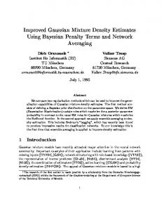
Figure 2: The curve of position error.

Figure 1: Comparison of the trajectory estimations. Table 2: RMSE and time of different algorithms.

4.1.2. Simulation Results and Analysis. We compare the performances of GMEKF, GMUKF, GMCKF, and IGMCKF algorithms with the conditions mentioned above. Figure 1 shows the results of the trajectory estimations of the target from the different algorithms versus the truth trajectory. Figure 2 shows the position error of different algorithms, and Figure 3 compares the position errors in 𝑋 direction and 𝑌 direction among the different algorithms. In Figure 1, the red dotted-dashed line denotes the trajectory of observation station, and the arrow denotes the movement heading. From Figure 2, it can be observed that the GMEKF and GMUKF have bad stability, and the error can be up to 25 m. The performance improvement of GMCKF is much better, and the error could be up to 13 m. The IGMCKF has the best tracking performance with an error up to 10 m, and the error could be limited to 3 m during stabilization. Figure 4 shows the tracking performance of target velocity of different algorithms. Figure 5 shows the tracking performance of velocity components in 𝑋 direction and 𝑌 direction, respectively. From Figure 4, it can be observed that the GMCKF algorithm could track the target velocity after about 30 s, while the other algorithms need about 80 s. Figure 6 shows the comparison of velocity errors of different algorithms. Figure 7 shows the comparison of target headings of different algorithms. The accuracy achieved by the filtering methods was analyzed using the following metrics. The Root-Mean-Square Error (RMSE) is defined as

RMSE = √

1

𝑡step

2

2

̂ 𝑘 ) + (𝑦𝑘 − 𝑦 ̂ 𝑘 ) ), ∑ ((𝑥𝑘 − 𝑥 𝑡step 𝑘=1

(36)

NCI 1.1534 0.7591 0.6522 0.6280

GMEKF GMUKF GMCKF IGMCKF

RMSE (m) 6.3300 5.4350 3.9051 2.0042

Time (ms) 36.105 130.631 163.330 257.302

̂𝑘) where 𝑡step is the simulation steps and (𝑥𝑘 , 𝑦𝑘 ) and (̂ 𝑥𝑘 , 𝑦 are the true position and estimated position, respectively, of target at time 𝑘. The average Noncredibility Index (NCI) [25, 26] is defined as NCI =

1

2

𝑡step

∑ [10 ln (

𝑡step 𝑘=1

[ 2

− 10 ln (

2

̂ 𝑘 ) + (𝑦𝑘 − 𝑦 ̂𝑘) ) ((𝑥𝑘 − 𝑥 𝑃𝑝,𝑘

RMSE

(37)

2

̂ 𝑘 ) + (𝑦𝑘 − 𝑦 ̂𝑘) ) ((𝑥𝑘 − 𝑥

)

)] , ]

where 𝑃𝑝,𝑘 is the uncertainty information of the position 2 + 𝑃2 . estimation and 𝑃𝑝,𝑘 = √𝑃𝑥,𝑘 𝑦,𝑘 Table 2 gives the NCI, RMSE, and the computing time cost of different tested algorithms. From Table 2, we can see that IGMCKF has the smallest RMSE which illuminates that the algorithm has the highest precision. The running time of IGMCKF is the longest because IGMCKF needs to update the weight during the time update stage and split the observation noise into several Gaussian components and merge them based on CKF estimating the cubature points. But the running time could satisfy the requirement of real-time target tracking. The NCI of the algorithms except the GMEKF are below 1, which

7

20 10 0 −10

0

50

100

GMEKF GMUKF

150 Time (s)

200

250

300

Position error on Y (m)

Position error on X (m)

Discrete Dynamics in Nature and Society 30 20 10 0 −10

0

50

100

150 Time (s)

GMEKF GMUKF

GMCKF IGMCKF

200

250

300

GMCKF IGMCKF

Figure 3: The curve of position error in 𝑋 and 𝑌. 3

are set as follows: [1 [ [0 [ [ [0 [ 𝐹=[ [ [0 [ [ [0 [ [0

Velocity (m/s)

2.5 2 1.5 1 0.5 0

0

50

Real velocity GMEKF GMUKF

100

150 Time (s)

200

250

300

GMCKF IGMCKF

Figure 4: The tracking curve of target velocity.

illuminate that the credibility of the various filter algorithms is high. 4.2. Simulation 2 4.2.1. Simulation Parameter. We will compare the performance of proposed algorithm (interacting multiple model CKF, IMMCKF) and interacting multiple model Gaussian mixture CKF (IMMGMCKF) algorithms. The filter parameters are set as follows. The initial position of target is (20, 150), the initial velocity is (0, −1.5) m/s, and the acceleration is 0 m/s2 . The target moves with constant initial velocity in a straight line from 0 s to 100 s. Then it maneuvers and moves with constant acceleration (0.0075, 0.0075) m/s2 from 101 s to 200 s. From 201 s to 300 s, it moves with constant velocity (0.7575, −0.7425) m/s. From 301 s to 380 s, it maneuvers with constant acceleration (−0.025, −0.015) m/s2 , and it moves with constant velocity (−1.2175, −1.9275) m/s for the last 20 s. The observation noise is set the same as simulation 1. Singer model is employed for the IGMCKF algorithm, the ̈ and other filter parameters state vector is 𝑥 = [𝑥, 𝑥,̇ 𝑥,̈ 𝑦, 𝑦,̇ 𝑦],

10 [ [10 [ [ [10 𝑃0 = [ [0 [ [ [0 [ [0 1 [ 20 [ [1 [ [8 [ [1 [ [ 𝑄=[6 [0 [ [ [ [0 [ [ [ 0 [ 𝑅=[

𝑇2 0 0 2 1 𝑇 0 0

𝑇 0

1 0 0

0

0 1 𝑇

0

0 0 1

0

0 0 0

0] ] 0] ] ] 0] ] ], 2] 𝑇 ] 2] ] 𝑇] ] 1]

10 10 0

0

20 30 0

0

30 60 0

0

0

0 10 10

0

0 10 20

0

0 10 30

1 8 1 3 1 2 0

1 6 1 2

0

] 0] ] ] 0] ], 10] ] ] 30] ] 60]

0

0 0

0

0

0 1 0 20 1 0 0 8 1 0 0 6

0 1 8 1 3 1 2

1

(38)

] ] ] 0] ] ] ] 0] ] , 1] ] ] 6] 1] ] ] 2] ] 1 ]

10 0

]. 0 10

For the IMMCKF and IMMGMCKF algorithms, three models are employed: two constant acceleration models with different acceleration and constant velocity model. The model initial distribution is 𝑢 = [0.8, 0.1, 0.1], and Markov transition matrix is as follows: 0.95 0.025 0.025 [0.025 0.95 0.025] (39) Π=[ ]. [0.025 0.025 0.95 ]

Discrete Dynamics in Nature and Society 4

Velocity on Y (m/s)

Velocity on X (m/s)

8

2 0 −2 −4

0

50

100

Real GMEKF GMUKF

150 Time (s)

200

250

300

4 2 0 −2 −4

0

50

100

150 Time (s)

Real GMEKF GMUKF

GMCKF IGMCKF

200

250

300

GMCKF IGMCKF

1

Velocity error on Y (m/s)

Velocity error on X (m/s)

Figure 5: The tracking curve of velocity components.

0 −1 −2

0

50

100

GMEKF GMUKF

150 Time (s)

200

250

300

1 0 −1 −2 −3

0

50

100

GMEKF GMUKF

GMCKF IGMCKF

150 Time (s)

200

250

300

GMCKF IGMCKF

Figure 6: The curve of velocity error.

200

150

150

100 50

100 Heading ( ∘ )

0 50

−50

0

Y −100

−50

−150 −200

−100

−250

−150 −200

−300 0

50

100

150

200

250

300

−350

0

50

Real heading GMEKF GMUKF

GMCKF IGMCKF

100

150

X

Time (s) Real IMMCKF

IMMGMCKF IGMCKF

Figure 8: Comparison of the trajectory estimations.

Figure 7: The estimation curve of target heading.

4.2.2. Simulation Results and Analysis. The simulation results are obtained from 50 Monte Carlo runs. Figure 8 shows the position trajectory of various algorithms. Figures 9 and 10 denote the RMSE of position tracking in 𝑋 direction and 𝑌 direction, respectively. Figures 11 and 12 denote the RMSE of velocity tracking in 𝑋 direction and 𝑌 direction, respectively. From the above simulation results and Table 3, it can be seen that the IMMCKF has the worst accuracy of estimation,

and because of that the observation noise is modelled as glint noise, and the IMMCKF algorithm is suitable for the Gaussian noise. The IMMGMCKF and IGMCKF have the similar accuracy of estimation and because of that the Gaussian mixture algorithm could deal with the non-Gaussian noise well. The running time of the IMMGMCKF is the longest and because of that the algorithm needs to switch between different motion models. The proposed algorithm has the best

Discrete Dynamics in Nature and Society

9

Table 3: Comparisons of average RMSE and running time of different algorithms.

IMMCKF IMMGMCKF IGMCKF

𝑋 position (m) 0.6713 0.1074 0.0983

𝑌 position (m) 0.6909 0.1238 0.0895

𝑋 velocity (m/s) 0.4741 0.0909 0.0463

1.4

1.6

1.2

1.4

X velocity RMSE

X position RMSE

Running time (ms) 222 315 182

1.2

1 0.8 0.6

1 0.8 0.6

0.4

0.4

0.2

0.2

0

𝑌 velocity (m/s) 0.4930 0.0920 0.0462

0 0

50

100

150

200 Steps

250

300

350

400

0

50

100

150

200 Steps

250

300

350

400

300

350

400

IMMCKF IMMGMCKF IGMCKF

IMMCKF IMMGMCKF IGMCKF

Figure 11: X velocity RMSE. Figure 9: X position RMSE. 1.4 1

1.2

0.9 1 Y velocity RMSE

0.8 Y position RMSE

0.7 0.6 0.5

0.6 0.4

0.4 0.3

0.2

0.2

0

0.1 0

0.8

0

50

100

150

200 Steps

250

300

350

400

IMMCKF IMMGMCKF IGMCKF

0

50

100

150

200 Steps

250

IMMCKF IMMGMCKF IGMCKF

Figure 12: Y velocity RMSE.

Figure 10: Y position RMSE.

5. Conclusion estimation accuracy and best computation complexity and could satisfy the real-time target tracking requirement.

An alternative efficient nonlinear filtering algorithm is designed in this paper, which is an improved Gaussian mixture filter within the Cubature Kalman Filter frame. The

10 algorithm could deal with the nonlinear filtering problem with non-Gaussian noise using Gaussian mixture density approximating the observation noise and update the weight adaptively with integral square difference during the time update stage. The feasibility of the algorithm was proven using a simulation based on the target tracking on offing, and the simulation shows that the proposed algorithm has higher estimation precision and faster tracking response.

Competing Interests The authors declare that there are no competing interests.

References [1] Y. Bar-Shalom, X. R. Li, and T. Kirubarajan, Estimation with Applications to Tracking and Navigation: Theory Algorithms and Software, John Wiley & Sons, New York, NY, USA, 2001. [2] O. Levent and F. A. Aliev, “Comment on ‘adaptive fading Kalman filter with an application’,” Automatica, vol. 34, no. 12, pp. 1663–1664, 1998. [3] D. H. Zhou and P. M. Frank, “Strong tracking filtering of nonlinear time-varying stochastic systems with coloured noise: application to parameter estimation and empirical robustness analysis,” International Journal of Control, vol. 65, no. 2, pp. 295– 307, 1996. [4] M. Nørgaard, N. K. Poulsen, and O. Ravn, “New developments in state estimation for nonlinear systems,” Automatica, vol. 36, no. 11, pp. 1627–1638, 2000. [5] M. Norgaard, K. N. Poulsen, and O. Ravn, Advances in Derivative-Free State Estimation for Nonlinear Systems, Department of Mathematical Modeling, Technical University of Denmark, Kongens Lyngby, Denmark, 2000. [6] S. J. Julier and J. K. Uhlmann, “Unscented filtering and nonlinear estimation,” Proceedings of the IEEE, vol. 92, no. 3, pp. 401– 422, 2004. [7] W. Fan and Y. Li, “Accuracy analysis of sigma-point Kalman filters,” in Proceedings of the Chinese Control and Decision Conference (CCDC ’09), pp. 2883–2888, Guilin, China, June 2009. [8] X.-X. Wang, L. Zhao, Q.-X. Xia, W. Cao, and L. Li, “Design of unscented Kalman filter with correlative noises,” Control Theory & Applications, vol. 27, no. 10, pp. 1362–1368, 2010. [9] W. Xiaoxu, Z. Lin, and P. Quan, “Design of UKF with correlative noises based on minimum mean square error estimation,” Control and Decision, vol. 25, no. 9, pp. 1393–1398, 2010. [10] K. Ito and K. Xiong, “Gaussian filters for nonlinear filtering problems,” IEEE Transactions on Automatic Control, vol. 45, no. 5, pp. 910–927, 2000. [11] I. Arasaratnam and S. Haykin, “Cubature Kalman filters,” IEEE Transactions on Automatic Control, vol. 54, no. 6, pp. 1254–1269, 2009. [12] A. Dhital, Bayesian Filtering for Dynamic Systems with Applications to Tracking, Universitat Politecnica de Ctalunya, Barcelona, Spain, 2010. [13] B. Jia, M. Xin, and Y. Cheng, “High-degree cubature Kalman filter,” Automatica, vol. 49, no. 2, pp. 510–518, 2013. [14] O. Cappe, S. J. Godsill, and E. Moulines, “An overview of existing methods and recent advances in sequential Monte Carlo,” Proceedings of the IEEE, vol. 95, no. 5, pp. 899–924, 2007.

Discrete Dynamics in Nature and Society [15] D. L. Alspach and H. W. Sorenson, “Nonlinear Bayesian estimation using Gaussian sum approximations,” IEEE Transactions on Automatic Control, vol. 17, no. 4, pp. 439–448, 1972. [16] G. Terejanu, P. Singla, T. Singh, and P. D. Scott, “Adaptive Gaussian sum filter for nonlinear Bayesian estimation,” IEEE Transactions on Automatic Control, vol. 56, no. 9, pp. 2151–2156, 2011. [17] X. Y. Fu and Y. M. Jia, “An improvement on resampling algorithm of particle filters,” IEEE Transactions on Signal Processing, vol. 58, no. 10, pp. 5414–5420, 2010. [18] N. Kabaoglu, “Target tracking using particle filters with support vector regression,” IEEE Transactions on Vehicular Technology, vol. 58, no. 5, pp. 2569–2573, 2009. [19] P. H. Leong, S. Arulampalam, T. A. Lamahewa, and T. D. Abhayapala, “A Gaussian-sum based cubature Kalman filter for bearings-only tracking,” IEEE Transactions on Aerospace and Electronic Systems, vol. 49, no. 2, pp. 1161–1176, 2013. [20] Y.-B. Kong and X.-X. Feng, “Passive target tracking algorithm based on improved gaussian mixture particle filter,” Modern Radar, vol. 34, no. 7, pp. 44–50, 2012. [21] G. Terejanu, P. Singla, T. Singh, and P. D. Scott, “Uncertainty propagation for nonlinear dynamic systems using gaussian mixture models,” Journal of Guidance, Control, and Dynamics, vol. 31, no. 6, pp. 1623–1633, 2008. [22] G. Terejanu, P. Singla, T. Singh, and P. D. Scott, “A novel Gaussian sum filter method for accurate solution to the nonlinear filtering problem,” in Proceedings of the 11th International Conference on Information Fusion (FUSION ’08), pp. 1–8, Cologne, Germany, July 2008. [23] J. L. Williams and P. S. Maybeck, “Cost-function-based Gaussian mixture reduction for target tracking,” in Proceedings of the 6th International Conference on Information Fusion (FUSION ’03), pp. 1047–1054, IEEE, Queensland, Australia, July 2003. [24] G. Terejanu, “An adaptive split-merge scheme for Uncertainty propagation using Gaussian mixture models,” in Proceedings of the 49th AIAA Aerospace Sciences Meeting including the New Horizons Forum and Aerospace Exposition, Orlando, Fla, USA, January 2011. [25] X. R. Li and Z. Zhao, “Measuring estimator’s credibility: noncredibility index,” in Proceedings of the 9th International Conference on Information Fusion (FUSION ’06), pp. 1–8, IEEE, Florence, Italy, July 2006. [26] R. P. Blasch, A. Rice, and C. Yang, Nonlinear Track Evaluation Using Absolute and Relative Metrics, The International Society for Optical Engineering, 2006.

Advances in

Operations Research Hindawi Publishing Corporation http://www.hindawi.com

Volume 2014

Advances in

Decision Sciences Hindawi Publishing Corporation http://www.hindawi.com

Volume 2014

Journal of

Applied Mathematics

Algebra

Hindawi Publishing Corporation http://www.hindawi.com

Hindawi Publishing Corporation http://www.hindawi.com

Volume 2014

Journal of

Probability and Statistics Volume 2014

The Scientific World Journal Hindawi Publishing Corporation http://www.hindawi.com

Hindawi Publishing Corporation http://www.hindawi.com

Volume 2014

International Journal of

Differential Equations Hindawi Publishing Corporation http://www.hindawi.com

Volume 2014

Volume 2014

Submit your manuscripts at http://www.hindawi.com International Journal of

Advances in

Combinatorics Hindawi Publishing Corporation http://www.hindawi.com

Mathematical Physics Hindawi Publishing Corporation http://www.hindawi.com

Volume 2014

Journal of

Complex Analysis Hindawi Publishing Corporation http://www.hindawi.com

Volume 2014

International Journal of Mathematics and Mathematical Sciences

Mathematical Problems in Engineering

Journal of

Mathematics Hindawi Publishing Corporation http://www.hindawi.com

Volume 2014

Hindawi Publishing Corporation http://www.hindawi.com

Volume 2014

Volume 2014

Hindawi Publishing Corporation http://www.hindawi.com

Volume 2014

Discrete Mathematics

Journal of

Volume 2014

Hindawi Publishing Corporation http://www.hindawi.com

Discrete Dynamics in Nature and Society

Journal of

Function Spaces Hindawi Publishing Corporation http://www.hindawi.com

Abstract and Applied Analysis

Volume 2014

Hindawi Publishing Corporation http://www.hindawi.com

Volume 2014

Hindawi Publishing Corporation http://www.hindawi.com

Volume 2014

International Journal of

Journal of

Stochastic Analysis

Optimization

Hindawi Publishing Corporation http://www.hindawi.com

Hindawi Publishing Corporation http://www.hindawi.com

Volume 2014

Volume 2014