Simulation of Large-Scale HPC Architectures Ian S. Jones and Christian Engelmann Computer Science and Mathematics Division Oak Ridge National Laboratory Oak Ridge, TN, USA
[email protected],
[email protected]
Abstract—The Extreme-scale Simulator (xSim) is a recently developed performance investigation toolkit that permits running high-performance computing (HPC) applications in a controlled environment with millions of concurrent execution threads. It allows observing parallel application performance properties in a simulated extreme-scale HPC system to further assist in HPC hardware and application software co-design on the road toward multi-petascale and exascale computing. This paper presents a newly implemented network model for the xSim performance investigation toolkit that is capable of providing simulation support for a variety of HPC network architectures with the appropriate trade-off between simulation scalability and accuracy. The taken approach focuses on a scalable distributed solution with latency and bandwidth restrictions for the simulated network. Different network architectures, such as star, ring, mesh, torus, twisted torus and tree, as well as hierarchical combinations, such as to simulate network-on-chip and network-on-node, are supported. Network traffic congestion modeling is omitted to gain simulation scalability by reducing simulation accuracy. Keywords-high-performance computing; parallel discrete event simulation; hardware/software co-design; performance evaluation; Message Passing Interface;
I. I NTRODUCTION On the road toward multi-petascale and exascale highperformance computing (HPC), the trend in system architecture goes clearly in only one direction. HPC systems are expected to dramatically scale up in compute node and processor core counts. According to the roadmap of the International Exascale Software Project (see http://www.exascale.org), an exascale computing system may have up to 1,000,000 compute nodes with 1,000 cores per node by 2018. Investigating performance and fault resilience of parallel applications at such an extreme scale (up to 1 billion concurrent threads for exascale) is impossible with today’s debugging, tracing and profiling tools. The recently developed Extreme-scale Simulator (xSim) [1], [2], is a new application performance investigation toolkit that allows to run a parallel application in a controlled environment at extreme scale. It permits observing performance properties in a simulated HPC system with millions of concurrent execution threads to further assist in HPC hardware and scientific application software co-design. While traditional debugging and performance tools rely on instrumentation and monitoring,
xSim focuses on an alternative approach using a lightweight parallel discrete event simulation (PDES) that provides an HPC application execution environment with a virtual wall clock time. A Message Passing Interface (MPI) application can be executed in a highly oversubscribed mode at extreme scale on today’s HPC systems and its performance properties can be evaluated based on virtual wall clock timing, instrumentation, monitoring, and a simple, efficient architectural system model. While simulation approaches have been used in the past (see Section II), they did not scale to millions of concurrent threads and they did not provide the needed amount of simulation accuracy at scale. The xSim simulation toolkit is designed to handle such high thread counts and to provide enough accuracy to identify performance properties. xSim itself is designed like a traditional performance investigation tool, as an interposition library that sits between the MPI application and the MPI layer, using the MPI performance tool interface (PMPI). It intercepts MPI calls from the application to hide all PDES-related mechanisms, such as virtual time management, virtual process messaging, maintaining causality, and virtual processes management. Each virtual MPI process is encapsulated in a user-space thread that has its own virtual time, while messages between virtual MPI processes are sent and received via the PDES layer. xSim supports a basic set of MPI functions and is able to run C and Fortran MPI applications. An application is run in the simulator using the following steps: • •
•
Add “#include xsim-c.h” to the C source code, or add “#include xsim-f.h” to the Fortran source code. Recompile the application and link it with the xsim library, e.g., “-lxsim”, and the respective xsim programming language interface library, e.g, “-lxsim-c” for C or “-lxsim-f” for Fortran Run the application with “mpirun -np -xsim-np ”
The current implementation [1], [2] is able to scale a basic MPI hello world program to up to 1 million virtual MPI processes on a small 4-node compute cluster with 2 processor cores per node and 8GB total RAM, using 4GB RAM just for virtual process stack. This extremely high ratio
of virtual-to-native threads, 125,000 in this case, is due to the light-weight implementation of virtual threads and of the PDES layer. xSim is also capable of investigating the performance of basic computational MPI applications to up to 16,384 virtual processors on the same system, i.e., with virtual-to-native threads ratio of 2,048. This paper focuses on one of the deficiencies of this prototype, the network model. The PDES-driven simulation accounts for the execution time for each virtual MPI process using the actual execution time on the real processor scaled by a processor model. It also accounts for the wait time incurred by communication for each virtual MPI process using a network model. The current implementation of the network model accounts for latency and bandwidth restrictions in a basic star network architecture only. Most HPC systems, however, have more complex network architectures, such as the 3-D twisted torus network in the Cray XT series [3]. This paper presents a newly developed network model for the xSim performance investigation toolkit that is capable of providing simulation support for a variety of network architectures with the appropriate trade-off between simulation scalability and accuracy. The solution extends the existing scalable distributed solution for latency and bandwidth restrictions in a star network to other simulated network architectures, such as ring, mesh, torus, twisted torus, and tree, as well as to hierarchical combinations, e.g., to simulate network-on-chip and network-on-node. As modeling traffic congestion with millions of virtual network links is too extensive in practice, it is omitted to gain simulation scalability by reducing simulation accuracy. This paper is structured as follows. Section II summarizes further related work and Section III presents the overall technical approach. Section IV details the design of the prototype implementation and Section V presents the obtained experimental results. Section VI concludes this paper with a short summary of the presented work and a brief discussion about ongoing and future work. II. R ELATED W ORK Discrete event simulation (DES) has been used in the past, such as in computer system design, molecular dynamics research and military battle field analysis, for investigating the behavior of a complex system consisting of many interacting entities. The operation of a complex system is represented as a chronological sequence of events and corresponding system state changes, allowing to stop, compress and expand the virtual time of the simulated state machine. A PDES [4], [5] is a parallel implementation of a DES that additionally maintains causality as state transitions are executed simultaneously in the parallel execution threads of the simulated state machine. In 2001, the Java Cellular Architecture Simulator (JCAS) [6] was developed as part of a collaboration between
Oak Ridge National Laboratory (ORNL) and IBM to investigate scalable and fault-tolerant scientific algorithms for large-scale HPC systems planned at that time, such as the 100,000-processor IBM Blue Gene/L. The final prototype was able to run up to 500,000 virtual processes on a Linux cluster with 5 native processors (1 for visualization and 4 for computation) solving basic mathematical problems, like Laplace’s equation and global maximum search. While it was able to run algorithms at scale, it lacked certain important features, such as time-accurate simulation, high performance, support for running the simulator on atop MPI, and a fully functional virtual MPI. Nevertheless, the JCAS project sparked a new area of research in scalable and fault-tolerant algorithms [7], [8], [9]. xSim is the de-facto successor of the JCAS project aiming at a better performing and more accurate implementation. Also in 2001, the BigSim [10] project (see http://charm.cs.uiuc.edu/research/bigsim) was initiated at the University of Illinois at Urbana-Champaign by the IBM Blue Gene/C project to study programming issues in large-scale HPC systems. The BigSim Emulator is meant for application testing and debugging at scale and is build atop Charm++ and Adaptive MPI [11]. It supports up to 100,000 virtual MPI processes distributed over 2,000 native processors. Similar to JCAS, the BigSim Emulator does not offer time-accurate simulation. While it provides more functionality than JCAS, such and a fully functional virtual MPI, it scales worse due to the Charm++/AMPI layer. The BigSim Simulator is meant for identification of performance bottlenecks, such as load imbalances, communication contention and long critical paths. It is a trace-driven PDES that models architectural parameters of a HPC system. For time-accurate simulation, it supports a variable-resolution processor model, ranging from simple scale factors to interpolation based on performance counters, and a simple or detailed model of the entire communication fabric. While the BigSim Simulator uses a PDES to maintain accuracy, it does not support running native applications. The xSim project aims at providing a solution that offers the advantages of both, the BigSim Emulator and Simulator, with a time-accurate, scalable and light-weight PDES solution. Other trace-driven PDES solutions for investigating parallel application performance include DIMEMAS [12], which processes traces from MPIDTrace and generates trace files that are suitable for the two performance analysis tools, PARAVER and Vampir. Recently developed at ORNL, µπ [13] is a PDES-based system for predicting the performance of parallel programs. It aims at different methods for interfacing native applications with the virtual system created by a PDES layer, such as source code, library (currently implemented) and virtual machine grafting. µπ is based on the µsik PDES engine (see http://kalper.net/kp/software/musik), which sup-
ports conservative and optimistic execution. A prototype was recently tested on 216,000 cores of the Jaguar Cray XT5 at ORNL, providing over 27 million virtual MPI ranks, each with its own thread context, and all ranks fully synchronized by virtual time. µπ’s virtual process implementation relies on an operating system (pthread) thread for each virtual MPI rank, which inherently causes a significant performance loss. µπ requires an extreme-scale system to simulate an extreme-scale system. For example, the ratio of virtual-tonative threads is only 125 in the 27 million run. In contrast, the BigSim Emulator achieved a factor of 50 about 10 years ago and JCAS offered 100,000, both without a PDES. xSim is far more advanced in terms of scalability (virtual-to-native ratio of up to 125,000) and usability (46 MPI calls). µπ currently does not implement a processor or network model. Also a recent development, the Structural Simulation Toolkit (SST) from Sandia National Laboratories [14], [15] offers cycle-accurate simulation of novel compute-node architectures, including processor, memory, and network. SST is a modular PDES framework on top of MPI and scales only to a few nodes for cycle-accurate simulation or to a few hundred nodes with more relaxed accuracy. Its value is in the capability to investigate the performance features of future architectures in detail and to generate application models for larger-scale simulations, similar to the BigSim Emulator/Simulator combination. The work in this paper aims to facilitate this synergy between smallscale cycle-accurate and large-scale communication-accurate simulations. Ongoing efforts beyond this paper focus on integrating SST and xSim, such that SST can take advantage of the scalability of the xSim solution and xSim is able to utilize different processor and network models via the SST implementation. SST and xSim were originally developed as part of the U.S. Department of Energy’s Institute for Advanced Architecture and Algorithms (IAA) (see http://www.csm.ornl.gov/iaa). It was established in 2008 to facilitate the co-design of architectures and applications in order to create synergy in their respective evolutions for closing the application-architecture performance gap. The IAA currently targets the development of architecture-aware algorithms and the supporting runtime features needed by these algorithms to solve general sparse linear systems common in many scientific applications. It also focuses on evaluating the algorithmic impact of future HPC system architecture choices. There are a variety of detailed network architecture simulators, such as ns2/ns3 [16] and [17] and NetSim [18], that are able to provide network performance metrics at various abstraction levels, such as network, sub-network, and packet traces. These detailed network architecture simulators offer high-accuracy/low-scalability results that are not compatible with the low-accuracy/high-scalability approach taken in this paper.
III. T ECHNICAL A PPROACH As briefly described earlier, the general design of the xSim simulation toolkit is as follows. xSim sits between the MPI library and a parallel application as an interposition library. It intercepts MPI calls coming from the application via its own C/Fortran MPI application programming interface (API), i.e., xSim provides an MPI layer to the application while the native MPI layer is used by xSim via the PMPI API. The interposition library essentially wraps an MPI application into a virtual execution environment controlled by the xSim PDES. The user-space thread management of the PDES layer permits executing many virtual MPI processes within a single native MPI process, while maintaining a virtual time for each virtual MPI process. For example, the performance of basic computational MPI applications to up to 16,384 virtual MPI processes could be investigated on a 4-node cluster with 2 processor cores per node despite a 2,048times oversubscription in terms of real processor cores vs. virtual MPI processes [1]. The PDES-driven simulation uses a scaling processor model to account for the execution time for each virtual MPI process and a latency/bandwidth network model to account for the the wait time incurred by communication between virtual MPI processes. In order to create a meaningful concept of latency and bandwidth within the simulated HPC system, every communication between two virtual MPI processes has an associated cost, which reflects the time to transmit the message from the source to the destination. This message latency is proportional to the network distance between source and destination, i.e., proportional to the number of network links en-route to the destination. This network route depends on the network architecture and the routing protocol. The message latency is additionally influenced by the the network link bandwidth, i.e., the time to transmit a message of a certain size. The message latency L for a message size s and a network distance (hop count) h in a given network architecture with a link latency l and a link bandwidth b can be calculated as follows: L = (h ∗ l) + (s/b), where (h ∗ l) is the latency of the first byte transmitted between source and destination and (s/b) is the latency between the first and the last byte sent/received by the source/destination. The existing xSim prototype implements this network model just for the star network. The approach taken in this work is to implement additional network models for ring, mesh, torus and twisted torus network architectures based on the same concept for message latency. In hierarchical combinations, e.g., a two-dimensional torus network-on-chip with a two-dimensional mesh network-on-node with a three-dimensional twisted torus node network, message latency is calculated based on the number and type of links en-route. This includes considering the entry/exit points between the different networks, the different link latencies, and the lowest link bandwidth. As
hierarchical combinations are not supported by the existing xSim prototype, the approach taken in this work is to extend the network model to support this capability by providing the necessary functionality for specifying hierarchical network architecture combinations and for calculating network distance and minimum bandwidth for a message path across different connected networks. This simple, but powerful, approach for a network model does not account for traffic congestion at the intermediary links. As stated earlier, congestion modeling is currently not considered for the xSim toolkit as this would require it to accumulate and evaluate statistics for each link in a simulated system with millions of links. The network model could easily consume a significant portion of the xSim runtime, making it impossible to execute the simulation in the first place. This scalability/accuracy trade-off is inevitable as it takes a 10-100 exaflop system to accurately simulate a 1 exaflop supercomputer. IV. I MPLEMENTATION The prototype implementation containing the new network models and support for hierarchical combinations relies on a set of functions that provide the mathematical message latency model for the star, ring, mesh, torus, twisted torus and tree network architectures in a reentrant fashion. Every message transmitted between two virtual MPI processes is evaluated for its virtual network route and size. In addition to the timestamp containing the virtual time of the sending virtual MPI process, each message also has a timestamp containing the virtual time of the receiving virtual MPI process. The source timestamp is obtained from the PDES virtual time management and marks the virtual MPI process time the first byte is sent. The destination timestamp is calculated by the network model based on source timestamp, the architectural network parameters, and the source/destination locations. It marks the virtual MPI process time the last byte is received. A receiving virtual MPI process may need to wait (in virtual time) for a sending virtual MPI process to send the message. This virtual wait time is added. Conversely, a receiving virtual MPI process may not be ready yet to receive a message (in virtual time). In this case the virtual receive time is equal to the virtual MPI process time when the destination is ready. As the MPI standard does not define a progress model, the source is not hold up (in virtual time) by a destination that is not ready, i.e., the implemented network model defines its own asynchronous progress model. For causality, the PDES layer ensures that each virtual process receives/processes its messages in the receive time order as calculated by the network model.
Figure 1.
Figure 2.
Message route in a star topology.
Message route in a unidirectional ring topology.
via a command line parameter, i.e., -xsim-mn , and setup upon starting the simulation. In the following, the network model implementation for each topology is described in more detail. In the examples, node indices start with 0 and end with n − 1. 1) Star: The star topology (Figure 1) is modeled in a straightforward way as the number of hops h is always 2. The message latency L is simplified to (2 ∗ l) + (s/b), with a link latency l, a message size s and a link bandwidth b. 2) Ring: The unidirectional ring topology (Figure 2) is modeled in a similar way as the number of hops h is between 1 and n − 1 depending on source and destination location, where n is the number of nodes/links. A bidirectional ring topology cuts the maximum number of hops in half. The message latency L is calculated using the general network model L = (h ∗ l) + (s/b) described in Section III. 3) Mesh: A mesh topology (Figure 3) is a little more complex as the number of dimensions d and the size of each dimension m0 ,. . . ,md−1 needs to be specified upon setup. For example, a 27-node network may have a [3,3,3] configuration with 3 dimensions of size 3 each. For message latency calculation, source and destination location (virtual MPI ranks) are respectively translated into Euclidean coordinates. The route is determined by considering the respective coordinate for source and destination for each dimension in turn and summing up the number of hops h. The message latency L is calculated using the general network model described earlier. 4) Torus: The torus topology extends the mesh by additional links that loop around the edges of a dimension. The toroidal connectedness is an additional parameter for setting
A. Network Models In general, the simulated network architecture, including its topology and performance characteristics, is configured
Figure 3.
Message route in a mesh topology.
Figure 4.
A [3,3] torus with [0,1] (left) and [1,0] connectedness. Figure 8.
Message route in a twisted torus topology.
Figure 9. Figure 5.
up a virtual torus network that determines which, if any, dimensions are toroidal. For example, a 27-node network in a [3,3,3] configuration may have a [1,0,1] toroidal connectedness where dimension 0 and 2 loop around their edges. Figure 4 shows an example for a [3,3] torus. The message latency is calculated almost exactly in the same way as the mesh using the general network model L = (h ∗ l) + (s/b) by traversing each dimension using the source/destination Euclidean coordinates (Figure 5), with the exception that each toroidal dimension is treated like a ring (instead of a chain) when calculating the number of hops h.
Figure 6.
Figure 7.
Message route in a tree topology.
Message route in a torus topology.
A [3,3,2] twisted torus with toroidal degree 1 (left) and 2.
A [4,4] twisted torus with toroidal jump [1,2] (left) and [2,1].
5) Twisted Torus: The twisted torus is the most complex of all implemented network topology models. In addition to the torus parameters, a toroidal degree and a toroidal jump need to be specified for the virtual network setup as well. The toroidal degree is the dimension offset the looping link is connected to. For example, in a 27-node network with a [3,3,3] configuration, a toroidal connectedness [1,1,1] and a toroidal degree 1, dimension 0 loops around to 1, dimension 1 to 2, and 3 back to 0. If the toroidal degree is 2, dimension 0 loops around to 2, 1 to 0 and 3 to 2. Figure 6 shows an example for a [3,3,2] twisted torus. The toroidal jump is a vector specifying for each dimension the node offset for the looping link. For example, in a 27-node network with a [3,3,3] configuration, a toroidal connectedness [1,1,1], a toroidal degree 1 and a toroidal jump vector [1,2,3], looping around dimension 0 connects to the next node in dimension 1, looping around dimension 1 connects to the 2nd next node in dimension 2, and looping around dimension 3 connects to the 3rd next in dimension 0. Figure 7 shows an example for a [4,4] twisted torus. The message latency L in a twisted torus (Figure 8) is calculated using the general network model by traversing the dimensions from the source location toward the destination location to find the shortest path in a depth-first search fashion starting with the direction of travel with the lowest associated cost. A particular path is not searched further if a shorter one has already been found. The shortest path search is aborted and the path with the lowest hop count is chosen if all dimensions have been traversed at most once. While this is not an exhaustive search, it is accurate in the vast majority of situations. This accuracy/scalability trade-off is necessary to avoid a significant performance impact. 6) Tree: Lastly, the message latency L in a tree topology (Figure 9) is calculated by traversing first from the source up the tree branches to a common ancestor and then down
Figure 10.
Partitioning with 3 processors/node and 8 cores/processor.
the tree branches to the destination. Note that in contrast to all the previously described network topologies, not all nodes in the topology represent an actual processing element (compute node, processor or processor core). In fact, in HPC systems with tree architectures, such as a fat tree, only the leaf nodes are processing elements, while the other nodes are pure routers. Therefore, calculating the message latency L is relatively straightforward by considering source/destination location in the tree and the tree degree for the hop count h in the general network model L = (h ∗ l) + (s/b). B. Hierarchical Combinations To simulate a more accurate message latency between virtual MPI processes, combinations of networks are supported by hierarchically partitioning the simulated system (Figure 10). Each simulated network, such as the on-chip or on-node network, is encapsulated and modeled using its corresponding network model by abstracting each other (internal or external) network as a logical node. The message path is traversed for each network a message passes through using corresponding entry/exit points between networks. For example, a 1024 node system with a star topology may have 4 processors/node connected in a mesh topology, where each processor may have a 64-core network-on-chip mesh. Since the message latency L depends on network link latency l and bandwidth b, the accumulated latency (h ∗ l) and the minimum bandwidth bmin of all network links en-route is used in the general network model L = (h ∗ l) + (s/bmin ). V. E XPERIMENTAL R ESULTS The modified xSim toolkit with the newly developed network model was deployed on a 16-node Linux-based cluster. Each node has two 2.4GHz AMD Opteron processors with 4-cores each, i.e., 8 cores per node, and 8GB RAM, i.e., 1GB per core. The system with a total of 128 cores and 128 GB RAM is running Ubuntu 10.04.1 LTS. The network interconnect is non-blocking Gigabit Ethernet with a central switch, i.e, a star topology without switch congestion.
Figure 11. Simulator execution time running the random application with native process scaling (top) and virtual process scaling (bottom).
A. Micro Benchmarks The implementation was tested with two MPI programs. The first (ring), simply sends n messages containing a simple integer value around in a virtual MPI process ring, i.e., rank 0 to 1, ..., n − 1 to 0, such that each virtual MPI process receives the messages from all ranks. The second MPI program (random), sends the same number of messages, n2 , except that each message travels from a randomly selected source to a randomly selected destination, as opposed to the pattern seen in the ring communication. The ring MPI program is used to give an example of a specific communication pattern type and how this can affect the efficiency of various network types. The random MPI program is useful for obtaining average latencies, which suggest the general usefulness of a given network setup when used for a wide variety of applications. The first two series of experiments (Figure 11) tested the scalability of the xSim toolkit with the newly developed network model. In the first series, the simulator was scaled up from 2 to 128 native MPI processes (NPs) with 1 NP per native core on the test system and a fixed simulated 8 × 16 2-D mesh network topology using the random MPI application with 128 virtual MPI processes. In the second series, the random MPI application was scaled up from 256 to 65,536 virtual MPI processes (VPs) with a fixed 128 native MPI process count (again one per core) by respectively extending the 2-D mesh network topology. Each run was executed 10 times and the total execution time of the xSim toolkit was averaged over these 10 runs. From 2 to 128 NPs (with 128 VPs) the total execution time of the simulator shows the expected strong scaling as the same amount of work gets divided by more native MPI processes. From 256
Figure 12. Average MPI message latency L for virtual process scaling using the random application (top) and the ring application (bottom).
to 65,536 VPs (with 128 NPs) the total execution time of xSim experiences the expected impact of oversubscription. This performance impact is caused by the n2 number of messages that the random MPI application generates and that the PDES layer and the network model needs to handle. In both series of experiments, there is no observable performance difference between disabling the network model, using the old network model, or utilizing the new network model. This is expected as the old and the new network models are designed to have a very low computational impact. They do not require global synchronization or information exchange as modeling network congestion is omitted. The next two series of experiments (Figure 12) analyze the average MPI message latency L for all implemented network models using a generic version of every topology. These experiments provide a rough evaluation of the correctness of the implemented network model for each topology. The first, executes the random MPI application, varying the number of virtual MPI processes from 2 to 2,048. A corresponding 2-D topology is used for the mesh, torus and twisted torus networks, while the tree is configured as a corresponding
binary tree. The torus and twisted torus are completely toroidal in every dimension, i.e., their toroidal connectedness is [1. . . 1]). The twisted torus has a toroidal degree of 1, and a toroidal jump vector of [1. . . 1]. The virtual link latency l is set to 1 µs. The virtual link bandwidth b is set to 1 Gbps, which is an insignificant parameter value for these experiments as each message contains only one integer value. Each run was executed 10 times and the average MPI message latency L for each run was averaged over these 10 runs. In the second experiment, the ring MPI application is executed with the same parameters. Looking at the results for the random MPI application (Figure 12, top diagram), the star topology clearly outperforms all others as network contention at the central switch is not modeled. The next-best performing topology is the binary tree as its maximum network distance is 2log2 (n). The mesh, torus and twisted torus all show very similar results, with one point of interest. In squared √ √ particular setups, i.e., for n× n, the torus and twisted torus provide better performance than the mesh. The reason is that in a network of unequal dimensions, source and destination picked at random are statistically more likely to be further from the edges, meaning the advantage of having the edges loop around into one another becomes less significant. In a network of equal dimensions, this effect is reversed. The results for the ring MPI application (Figure 12, bottom diagram) show a different picture. The ring topology directly maps the application communication pattern, while the torus and twisted torus approximate the ring close enough to have similar performance. The constant performance of the star network can be observed again as congestion is not modeled. The mesh suffers from the missing loops around the edges of the torus and twisted torus. The binary tree performs worse due to the application communication pattern that simply forwards a message to the next MPI rank in-line, requiring traversing up and down the tree in a log2 -based fashion. The next experiment (Figure 13) involved varying the virtual link bandwidth b in a simulated 8 × 16 2-D mesh using the random MPI application. While each message only contains a single integer, significantly lowering the virtual link bandwidth b from 1Mbps to 0.1 bps should still have an impact on the average MPI message latency L. The performance tests executed and averaged with 10 runs per configuration confirm this behavior. The last experiment provides an example for examining hybrid topologies, such as multi-core processor systems. The investigation involves a 2-level hierarchical combination with one core-to-core communication network on each simulated processor and another processor-to-processor network. For simplicity, the same topology is used for both networks with different link latencies lprocessor and lcore , 1 and 0.1 µs respectively, and link bandwidths bprocessor and bcore , 1 and 10 Gbps respectively. The random MPI application is
Table I PARAMETERS OF THE SIMULATED NETWORKS Network Name None Ethernet x-core Ethernet (multi-core) Y x... Mesh Y xX... Mesh (dual-core) Y xX... Torus (dual-core) Y xX... Twisted Torus (dual-core)
Network Parameters No network model Star, 1Gbps, 25µs On processor: star, 12Gbps, 0.32µs Off processor: star, 1Gbps, 25µs 2D mesh, 8.8Gbps, 7µs On processor: star, 9.6Gbps, 0.32µs Off processor: 3D mesh, 8.8Gbps, 7µs On processor: star, 9.6Gbps, 0.32µs Off processor: 3D torus, 8.8Gbps, 7µs On processor: star, 9.6Gbps, 0.32µs Off processor: 3D twisted torus, 8.8Gbps, 7µs
Figure 13. Average MPI message latency L for different virtual link bandwidth b using the random application in a mesh.
Figure 15.
Figure 14. Average MPI message latency L for virtual process scaling using the random application and nested network topologies.
executed with a fixed 128 virtual MPI process count, while the number of simulated cores per simulated processor is varied. Figure 14 shows the results with the x axis listing the number of cores per processor with two sets of parentheses, indicating the configuration of the processor and core topology. The mesh, torus and twisted torus have almost identical sets of results. As the the number of cores per processor is increased, communication takes place predominantly within each processor, reducing the average MPI message latency to the core latency lcore . B. NAS Parallel Benchmarks The implementation was also tested with the NAS Parallel Benchmark (NPB) [19] suite. Table I details the different virtual network configurations used in the experiments. They are close to measured MPI performance on Gigabit Ethernet Linux clusters and Cray XT5 series supercomputers.
Simulator performance with the NAS EP benchmark.
The first series of experiments (Figure 15) evaluated the scalability of the xSim toolkit with the newly developed network model using the embarrassingly parallel (EP) benchmark. The experiments reveal that the simulator performance is actually better using the computationally intensive dual-core twisted torus network model than no network model at all. In both configurations, the number of virtual MPI messages is exactly the same (720,885 for 65,536 processes) and the number of virtual MPI process context switches is roughly the same (458,751 and 458,906 for 65,536 processes). However, the order these messages are being processed by the simulator is different due to the different virtual network configurations and xSim’s message processing based on receive time. Therefore, the overhead introduced by inserting messages into xSim’s ordered message queue, a red-black tree implementation, is different. In the second series of experiments using the NPB suite, the performance of the three-dimensional discrete Poisson V-cycle multigrid solver (MG) is evaluated in xSim with a standard Gigabit Ethernet configuration and different multicore configurations. Figure 16 shows that while the MG benchmark scales to some extend, the impact of the Gigabit Ethernet network becomes visible at 4096 virtual MPI processes. There is noticeably not much difference between the various multi-core configurations as the Gigabit Ethernet network is the main scalability limit.
Figure 16. Simulated performance of the NAS MG benchmark with a Gigabit Ethernet network and 1-16 cores per processor.
Figure 18. Simulated performance of the NAS MG benchmark with a dual-core 3D mesh, torus and twisted torus network.
VI. C ONCLUSIONS AND F UTURE W ORK
Figure 17. Simulated performance of the NAS MG benchmark with a 2D mesh network and a mesh width of 32, 64 and 128 processors.
The next series of experiments investigate the impact of network geometry on the MG benchmark. Figure 17 shows that there is practically no difference in using a 32-, 64- or 128-process wide 2D mesh network for this particular 3D multigrid solver. The comparison to the execution without a network model and to Figure 16 also reveals that the impact of increased latency in a 2D mesh is preventing any performance improvements by adding more processes. MG simply does not scale in this network setup. The last series of experiments targets a comparison of mesh, torus and twisted torus virtual network configurations. The MG benchmark is executed in a 3D network setup, where one dimension is increased and the other two remain at size 8. In addition each simulated processor has 2 cores. The twisted torus network jumps by 1 dimension in each dimension and wraps by 1 dimension. In Figure 18, the results clearly show that MG does not scale in a mesh network, but does scale in a torus or twisted torus network setup until 4096 virtual MPI processes. There is no difference between the torus and the twisted torus as the network diameter difference between both is not large enough.
We presented the implementation and performance results of a new virtual network model for the parallel application performance investigation toolkit xSim. The offered simulated HPC network architectures are star, ring, mesh, torus, twisted torus and tree. An additional capability is provided to combine different networks in a hierarchical manner to simulate network-on-chip and network-on-node. The implementation does trade off simulation accuracy by omitting network traffic congestion modeling to gain simulation scalability. The presented micro benchmark results show that the implementation performs as expected. The NPB results demonstrate the usability of the presented prototype. Further implementation details and more extensive results are available in a Master’s thesis [20]. The developed prototype has its limitations, such as the omitted traffic congestion modeling. The results show that the simulated network may have a lower than expected performance impact on the MPI application executed inside the simulator, as exemplified by the star network experiments. However, as it takes a 10-100 exaflop system to accurately simulate a 1 exaflop supercomputer, this scalability vs. accuracy tradeoff is inevitable. Performance investigations using this toolkit need to keep in mind this limitation. Future work in this area mostly focuses on validation of the implemented network model against existing networks using two strategies, model comparison, e.g., against more complex vendor-supplied models, and experimental comparison, e.g., using micro benchmarks and applications on production HPC systems. Further planned work looks at enhancing the network model capabilities with more advanced network topologies, such as Cray’s Dragonfly. ACKNOWLEDGMENT This research is sponsored by the Office of Advanced Scientific Computing Research; U.S. Department of Energy.
The work was performed at the Oak Ridge National Laboratory, which is managed by UT-Battelle, LLC under Contract No. De-AC05-00OR22725. The United States Government retains and the publisher, by accepting the article for publication, acknowledges that the United States Government retains a non-exclusive, paid-up, irrevocable, world-wide license to publish or reproduce the published form of this manuscript, or allow others to do so, for United States Government purposes.
[10] G. Zheng, G. Kakulapati, and L. V. Kale, “BigSim: A parallel simulator for performance prediction of extremely large parallel machines,” in Proceedings of the 18th IEEE International Parallel and Distributed Processing Symposium (IPDPS) 2004. Santa Fe, New Mexico: IEEE Computer Society, Apr. 26-30, 2004. [11] L. V. Kale, E. Bohm, C. L. Mendes, T. Wilmarth, and G. Zheng, “Programming petascale applications with Charm++ and AMPI,” in Petascale Computing: Algorithms and Applications, D. Bader, Ed. CRC Press, Dec. 2007, pp. 421–441.
R EFERENCES [1] C. Engelmann and F. Lauer, “Facilitating co-design for extreme-scale systems through lightweight simulation,” in Proceedings of the 12th IEEE International Conference on Cluster Computing (Cluster) 2010: 1st Workshop on Application/Architecture Co-design for Extreme-scale Computing (AACEC). Hersonissos, Crete, Greece: IEEE Computer Society, Sep. 20-24, 2010, pp. 1–8. [2] S. B¨ohm and C. Engelmann, “xSim: The extreme-scale simulator,” in Proceedings of the International Conference on High Performance Computing and Simulation (HPCS) 2011. Istanbul, Turkey: IEEE Computer Society, Los Alamitos, CA, USA, Jul. 4-8, 2011. [3] Cray Inc., Seattle, WA, USA, “Cray XT series system overview,” 2007. [4] R. M. Fujimoto, “Parallel discrete event simulation,” Communications of the ACM, vol. 33, no. 10, pp. 30–53, 1990. [5] K. S. Perumalla, “Parallel and distributed simulation: Traditional techniques and recent advances,” in Proceedings of the 38th Winter Simulation Conference 2006. Monterey, CA, USA: ACM Press, New York, NY, USA, 3-6, 2006, pp. 84– 95. [6] C. Engelmann and G. A. Geist, “Super-scalable algorithms for computing on 100,000 processors,” in Lecture Notes in Computer Science: Proceedings of the 5th International Conference on Computational Science (ICCS) 2005, Part I, vol. 3514. Atlanta, GA, USA: Springer Verlag, Berlin, Germany, May 22-25, 2005, pp. 313–320. [7] G. Bosilca, Z. Chen, J. Dongarra, and J. Langou, “Recovery patterns for iterative methods in a parallel unstable environment,” SIAM Journal on Scientific Computing (SISC), vol. 30, no. 1, pp. 102–116, 2007. [8] Z. Chen and J. J. Dongarra, “Algorithm-based checkpoint-free fault tolerance for parallel matrix computations on volatile resources,” in Proceedings of the 20st IEEE International Parallel and Distributed Processing Symposium (IPDPS) 2006. Rhodes Island, Greece: IEEE Computer Society, Apr. 25-29, 2006, p. 10. [9] H. Ltaief, E. Gabriel, and M. Garbey, “Fault tolerant algorithms for heat transfer problems,” Journal of Parallel and Distributed Computing (JPDC), vol. 68, no. 5, pp. 663–677, 2008.
[12] S. Girona, J. Labarta, and R. M. Badia, “Validation of dimemas communication model for MPI collective operations,” in Lecture Notes in Computer Science: Proceedings of the 7th European PVM/MPI Users‘ Group Meeting (EuroPVM/MPI) 2000, vol. 1908. Balatonf¨ured, Hungary: Springer Verlag, Berlin, Germany, Sep. 10-13 2000, pp. 39– 46. [13] K. S. Perumalla, “µπ: A highly scalable and transparent system for simulating MPI programs,” in Proceedings of the 3rdth International ICST Conference on Simulation Tools and Techniques (SIMUTools) 2010. Malaga, Spain: ACM Press, New York, NY, USA, Mar. 15-19, 2010. [14] Sandia National Laboratories, NM, USA, “Structural simulation toolkit (sst),” Available online at http://www.cs.sandia.gov/sst, 2011. [15] A. F. Rodrigues, K. S. Hemmert, B. W. Barrett, C. Kersey, R. Oldfield, M. Weston, R. Risen, J. Cook, P. Rosenfeld, E. CooperBalls, and B. Jacob, “The structural simulation toolkit,” SIGMETRICS Perform. Eval. Rev., vol. 38, pp. 37– 42, March 2011. [16] “Ns2 network simulator,” Available http://nsnam.isi.edu/nsnam, 2011.
online
at
[17] “Ns3 network simulator,” http://www.nsnam.org, 2011.
online
at
Available
[18] Tetcos, “Netsim network simulator,” Available online at http://tetcos.com/software.html, 2011. [19] Advanced Supercomputing Division, National Aeronautics and Space Administration (NASA), Ames, CA, USA, “NAS Parallel Benchmarks (NPB) documentation,” Available online at http://www.nas.nasa.gov/Resources/Software/npb.html, 2009. [20] I. S. Jones, “Simulation of large scale architectures on high performance computers,” Master’s thesis, Department of Computer Science, University of Reading, UK, Oct. 22, 2010.