Apollo mission that successfully put men on the surface of the moon and brought them safely back to ...... [3] A. C. Ducati, G. M. Giannini, and E. Muehlberger.
Simulation of MPD Flows Using a Flux-Limited Numerical Method for the MHD Equations
Kameshwaran Sankaran
A DISSERTATION PRESENTED TO THE FACULTY OF PRINCETON UNIVERSITY IN CANDIDACY FOR THE DEGREE OF MASTER OF SCIENCE IN ENGINEERING
RECOMMENDED FOR ACCEPTANCE BY THE DEPARTMENT OF MECHANICAL AND AEROSPACE ENGINEERING
January, 2001
Simulation of MPD Flows Using a Flux-Limited Numerical Method for the MHD Equations
Prepared by:
Kameshwaran Sankaran
Approved by:
Professor Edgar Y. Choueiri Dissertation Advisor
Professor Luigi Martinelli Dissertation Reader
Professor Stephen C. Jardin Dissertation Reader
c
Copyright by Kameshwaran Sankaran, 2000. All rights reserved.
Acknowledgments My experience, so far, as a graduate researcher, can be best described by the words of Sherlock Holmes: “They say that genius is an infinite capacity for taking pains. It’s a very bad definition, but it does apply to detective work.” Yet, in many ways it was also a very rewarding experience, and many people have played a role in helping it to be so. I chose to attend graduate school in Princeton largely due to a tradition of excellence in electric propulsion research, built by Prof. Robert Jahn. After I came here, Prof. Jahn taught me the fundamentals of the electric propulsion, and was always available to talk to me about “the big picture” of what research should be. Prof. Luigi Martinelli taught me the fundamentals of numerical methods and helped convince me that a new route to simulating plasma flows has to be taken. Prof. Steve Jardin taught me everything I know about computational plasma physics. He was around whenever I hit a wall (which I did frequently) and patiently guided me through the rough times. The most import role was that of my advisor Prof. Edgar Choueiri. I owe him a lot of thanks for giving me the opportunity to work on this problem, and persisting with me. He was as demanding in the lab as he was in the squash courts, and on both fronts I’ve only gotten better as a result of interacting with him. However, the best part of my grad school experience was working with the fellow graduate students. Invariably, they were my companions through the long hours in E-Quad. My discussions with them not only helped me pass the General Exam, but also contributed to much of my learning during this period. And of course, playing softball and squash with them was helpful in maintaining some sanity. Before this starts to resemble a speech at the Academy Awards, I’ll wrap it up with this: a friend told me a long time ago, “When you get a Bachelor’s degree, you’ll feel like you know everything; Then you go on for a Master’s degree and at the end of which you’ll feel like you know nothing; Then you go on for a Doctorate and ...”. I’ll complete the rest of the prophecy after I get a chance to verify the last part.
This dissertation carries the designation 3074-T in the records of the Department of Mechanical and Aerospace Engineering. i
Abstract
A new numerical scheme to accurately compute plasma flows of interest to propulsion was developed and validated first against standard test problems. The scheme treats the flow and the field in a self-consistent manner, and conserves mass, momentum, magnetic flux and energy. The characteristics-splitting scheme, which was developed from concepts used for the solution of Euler equations, was applied to solve the ideal MHD equations. The ability of this scheme to capture discontinuities monotonically was demonstrated. Flux-limited anti-diffusion was used to improve spatial accuracy away from discontinuities. Further improvements to the physical model, such as the inclusion of relevant classical transport properties, a real equation of state, multi-level equilibrium ionization models, anomalous transport, and multi-temperature effects, that are essential for the realistic simulation magnetoplasmadynamic flows, are implemented without affecting the underlying scheme. The solver, including the improved physical model, is then used to simulate plasma flow in a real magnetoplasmadynamic thruster configuration. The results of the simulation were found to to be in general agreement with experimental observations. They illustrate the need for using a real equation of state, instead of the ideal one, to enhance the realism and stability of the simulation. A multi-level equilibrium ionization model was found to give satisfactory results for species densities. The predicted value of thrust was found to be in excellent agreement with analytical predictions, though the predicted efficiency was significantly off, due to the lack of an electrode drop model.
ii
Nomenclature a
A
Br;�;z
B B��M
CA;F;S Dr; Dz e E E0
E Eg Ee;i Fconv Fdiff Hr; Hz j j; k Jmax kB k�th Lr; Lz me m_ Mtot Mprop Mi n_ e ne
n
p pe;i �p P
q
ra;c R; R
1
Sonic speed Jacobian of the hyperbolic system Radial, azimuthal and axial magnetic induction Magnetic induction vector Maxwell stress tensor Alfven, fast magnetosonic and slow magnetosonic velocity Numerical dissipation in the radial and axial flux directions Charge of an electron Electric field strength Effective electric field, as seen by the plasma Energy density of the plasma Gasdynamic energy density Internal energy density of electrons and heavy species Convective flux tensor Dissipative flux tensor Radial and axial flux across the cell face Current density Cell indices Total current Boltzmann’s constant Thermal conductivity tensor Flux limiters in the radial and axial directions Mass of an electron Propellant mass flow rate Initial spacecraft mass Propellant mass Atomic mass of propellant Net ionization/recombination rate Electron number density Unit normal Gasdynamic pressure Electron and heavy species pressure Isotropic pressure tensor Total pressure (magnetic pressure + gasdynamic pressure) Energy source/sinks Anode and cathode radius Matrix of eigenvectors, and its inverse
iii
Rm T Te Th
u U UnJ;K
ude ue VD vti Zeff
�r; �z �V �o �0 �th �� � �D �mfp
�
�o �vis �ei �AN � �e �res �equi ��vis !pe
e;i
j j j j
Magnetic Reynolds’ number Thrust Electron temperature Heavy species temperature Velocity vector Vector of conserved variables, �; �u; B; and E Value of U at time n � �t at the point (J � �r; K � �z ) Electron drift velocity Exhaust velocity E � B drift velocity Ion thermal velocity Average ionization fraction at a spatial location Ratio of specific heats Cell-size in the radial and axial direction Characteristic increment in spacecraft velocity permitivity of free space Classical resistivity Thrust efficiency Anisotropic resistivity tensor Eigenvalue Debye length Mean free path between collisions Diagonal matrix of eigenvalues Magnetic permeability of free space Coefficient of viscous dissipation Energy averaged momentum transfer collision frequency between electrons and ions Anomalous collision frequency Average density of the fluid Unbalanced charge density Residence time scale Time scale for energy equilibration between electrons and ions Viscous stress tensor Electron plasma frequency Electron, ion Hall parameter (ratio of gyro and collisional frequncies) Control volume in a mesh (cell) Volume of the cell j
iv
Contents Acknowledgments . . . . . . . . . . . . . . . . . . . . . . . . . . . . . . . . . . Abstract . . . . . . . . . . . . . . . . . . . . . . . . . . . . . . . . . . . . . . . Nomenclature . . . . . . . . . . . . . . . . . . . . . . . . . . . . . . . . . . . .
i ii iii
1 INTRODUCTION 1 1.1 Role of Plasma Propulsion . . . . . . . . . . . . . . . . . . . . . . . . . . 1 1.2 Motivation for This Thesis . . . . . . . . . . . . . . . . . . . . . . . . . . 6 1.3 Organization of This Thesis . . . . . . . . . . . . . . . . . . . . . . . . . . 12 2 PLASMA FLOW MODELING 2.1 Continuum Model of the Plasma . . . . . 2.2 Simplified Analytical Models . . . . . . . 2.3 Multidimensional Time-Dependent Model 2.3.1 Conservation of Mass . . . . . . 2.3.2 Conservation of Momentum . . . 2.3.3 Faraday’s Law . . . . . . . . . . 2.3.4 Conservation of Energy . . . . . 2.3.5 Equation of State . . . . . . . . . 2.3.6 Anomalous Transport . . . . . . . 2.3.7 Ionization Processes . . . . . . . 2.3.8 Summary of Governing Equations 2.3.9 Zero Divergence Constraint . . . 2.4 Summary . . . . . . . . . . . . . . . . .
. . . . . . . . . . . . .
. . . . . . . . . . . . .
. . . . . . . . . . . . .
. . . . . . . . . . . . .
. . . . . . . . . . . . .
. . . . . . . . . . . . .
. . . . . . . . . . . . .
. . . . . . . . . . . . .
. . . . . . . . . . . . .
. . . . . . . . . . . . .
. . . . . . . . . . . . .
. . . . . . . . . . . . .
. . . . . . . . . . . . .
. . . . . . . . . . . . .
. . . . . . . . . . . . .
. . . . . . . . . . . . .
. . . . . . . . . . . . .
14 14 16 19 20 20 22 24 28 30 31 34 34 35
3 NUMERICAL SOLUTION 3.1 Guiding Principles . . . . . . . . . . . . . . 3.2 Mesh System . . . . . . . . . . . . . . . . . 3.3 Consistency, Stability, and Convergence . . . 3.3.1 Lax-Wendroff Theorem . . . . . . . 3.3.2 Criteria for Stability and Convergence 3.4 Conservation Form . . . . . . . . . . . . . . 3.5 Hyperbolic (Convection) Equations . . . . . 3.5.1 Spatial Discretization . . . . . . . . .
. . . . . . . .
. . . . . . . .
. . . . . . . .
. . . . . . . .
. . . . . . . .
. . . . . . . .
. . . . . . . .
. . . . . . . .
. . . . . . . .
. . . . . . . .
. . . . . . . .
. . . . . . . .
. . . . . . . .
. . . . . . . .
. . . . . . . .
. . . . . . . .
36 36 37 40 41 41 44 46 46
v
. . . . . . . . . . . . .
. . . . . .
. . . . . .
. . . . . .
. . . . . .
. . . . . .
. . . . . .
. . . . . .
. . . . . .
. . . . . .
. . . . . .
. . . . . .
. . . . . .
. . . . . .
. . . . . .
. . . . . .
. . . . . .
49 50 54 54 55 56
4 MPD THRUSTER SIMULATIONS 4.1 Application of Governing Equations . . . . . . 4.2 Geometry . . . . . . . . . . . . . . . . . . . . 4.3 Boundary Conditions . . . . . . . . . . . . . . 4.3.1 Flow Properties . . . . . . . . . . . . . 4.3.2 Field Properties . . . . . . . . . . . . . 4.4 Initial Conditions . . . . . . . . . . . . . . . . 4.5 Schematic of Calculations . . . . . . . . . . . 4.6 Convergence and Stability Checks . . . . . . . 4.7 Results . . . . . . . . . . . . . . . . . . . . . . 4.7.1 Density . . . . . . . . . . . . . . . . . 4.7.2 Ionization Levels . . . . . . . . . . . . 4.7.3 Electron Temperatures . . . . . . . . . 4.7.4 Ion Temperatures . . . . . . . . . . . . 4.7.5 Velocities . . . . . . . . . . . . . . . . 4.7.6 Magnetic Field & Enclosed Current . . 4.7.7 Electric Field & Potential . . . . . . . 4.7.8 Hall Parameter & Anomalous Transport 4.7.9 Thrust & Efficiency . . . . . . . . . . . 4.8 Summary . . . . . . . . . . . . . . . . . . . .
. . . . . . . . . . . . . . . . . . .
. . . . . . . . . . . . . . . . . . .
. . . . . . . . . . . . . . . . . . .
. . . . . . . . . . . . . . . . . . .
. . . . . . . . . . . . . . . . . . .
. . . . . . . . . . . . . . . . . . .
. . . . . . . . . . . . . . . . . . .
. . . . . . . . . . . . . . . . . . .
. . . . . . . . . . . . . . . . . . .
. . . . . . . . . . . . . . . . . . .
. . . . . . . . . . . . . . . . . . .
. . . . . . . . . . . . . . . . . . .
. . . . . . . . . . . . . . . . . . .
. . . . . . . . . . . . . . . . . . .
. . . . . . . . . . . . . . . . . . .
57 57 59 61 61 63 64 65 67 69 69 69 71 72 72 73 75 76 77 79
. . . .
82 82 84 84 85
3.6
3.7
3.5.2 Temporal Discretization 3.5.3 Verification . . . . . . . Parabolic (Diffusion) Equations 3.6.1 Spatial Discretization . . 3.6.2 Temporal Discretization Summary . . . . . . . . . . . .
. . . . . .
. . . . . .
. . . . . .
. . . . . .
5 CONCLUDING REMARKS 5.1 What are the contributions of this thesis? 5.2 What remains to be done? . . . . . . . . 5.2.1 Computational Methods . . . . 5.2.2 Physical Models . . . . . . . . Bibliography
. . . . . .
. . . .
. . . . . .
. . . .
. . . . . .
. . . .
. . . .
. . . .
. . . .
. . . .
. . . .
. . . .
. . . .
. . . .
. . . .
. . . .
. . . .
. . . .
. . . .
. . . .
. . . .
89
A VECTOR OPERATIONS 95 A.1 IDENTITIES . . . . . . . . . . . . . . . . . . . . . . . . . . . . . . . . . 95 A.2 MANIPULATIONS . . . . . . . . . . . . . . . . . . . . . . . . . . . . . . 96
vi
B EIGENSYSTEM 97 B.1 Eigensystem of MHD . . . . . . . . . . . . . . . . . . . . . . . . . . . . . 97 B.1.1 rˆ Direction . . . . . . . . . . . . . . . . . . . . . . . . . . . . . . 98 B.1.2 zˆ Direction . . . . . . . . . . . . . . . . . . . . . . . . . . . . . . 99 C COMPUTER PROGRAM C.1 Main . . . . . . . . . . C.2 Declarations . . . . . . C.3 Memory Allocations . C.4 Input/Output . . . . . . C.5 Grid . . . . . . . . . . C.6 Initial Conditions . . . C.7 Boundary Conditions . C.8 Solve . . . . . . . . . C.9 Time Steps . . . . . . C.10 Convective Fluxes . . . C.11 Eigensystem . . . . . . C.12 Jacobian . . . . . . . . C.13 Linear Algebra . . . . C.14 Dissipative Fluxes . . . C.15 March in Time . . . . C.16 Species Energy . . . . C.17 Calculate Variables . .
. . . . . . . . . . . . . . . . .
. . . . . . . . . . . . . . . . .
. . . . . . . . . . . . . . . . .
. . . . . . . . . . . . . . . . .
. . . . . . . . . . . . . . . . .
. . . . . . . . . . . . . . . . .
. . . . . . . . . . . . . . . . .
vii
. . . . . . . . . . . . . . . . .
. . . . . . . . . . . . . . . . .
. . . . . . . . . . . . . . . . .
. . . . . . . . . . . . . . . . .
. . . . . . . . . . . . . . . . .
. . . . . . . . . . . . . . . . .
. . . . . . . . . . . . . . . . .
. . . . . . . . . . . . . . . . .
. . . . . . . . . . . . . . . . .
. . . . . . . . . . . . . . . . .
. . . . . . . . . . . . . . . . .
. . . . . . . . . . . . . . . . .
. . . . . . . . . . . . . . . . .
. . . . . . . . . . . . . . . . .
. . . . . . . . . . . . . . . . .
. . . . . . . . . . . . . . . . .
. . . . . . . . . . . . . . . . .
. . . . . . . . . . . . . . . . .
. . . . . . . . . . . . . . . . .
. . . . . . . . . . . . . . . . .
. . . . . . . . . . . . . . . . .
101 101 102 106 109 117 119 122 129 130 132 137 143 148 150 152 153 156
Chapter 1 INTRODUCTION The Earth is the cradle of the mind, but we cannot live forever in a cradle. Konstantin E. Tsiolkovsky
1.1 Role of Plasma Propulsion Arguably the greatest technological achievement of the twentieth century was NASA’s Apollo mission that successfully put men on the surface of the moon and brought them safely back to earth. However, only about 2% of the total mass of about 2750 metric tonnes of the rocket was useful payload. The bulk of the remaining mass was filled by the 960 thousand gallons of fuel needed for propulsion. The reason for the large propellant fraction is clear from the rocket equation, derived by Tsiolkovsky[1] in 1903. In the absence of external forces, the ratio of mass of propellant to the total mass of the rocket is given by the relation,
mprop =1 e mtot
�V=ue
where ue is the exhaust velocity of the propellant and increment imparted to the rocket. 1
;
(1.1)
�V is the characteristic velocity
Since the exhaust velocities of the chemical rockets used in the Saturn V were small (the F-1 engines used in the first stage had exhaust velocities ranging from 2600 to 3000 m/s from sea level to high altitude, and the J-2 engines used in the second and third stage had an exhaust velocity of 4200 m/s at high altitude) compared to the �V requirements for the mission, the mass of propellant required was enormous. Despite the advances in combustion research, the highest exhaust velocity of a functional chemical propulsion system, 3600 to 4500 m/s from sea level to high altitude (of the Space Shuttle Main Engine), is still inadequate for most deep-space missions of interest[2]. For missions beyond the moon, the
�V requirements indicate that chemical propulsion is not a practical solution, and a more viable alternative has to be used. Functionally, the inability of chemical propulsion systems to achieve higher exhaust velocities is due to the limitation in the maximum tolerable temperature in the combustion chamber, to avoid excessive heat transfer to the walls. Fundamentally, there is also an intrinsic limitation on the maximum energy that is available from the chemical reactions. Both these limitations can be overcome by the use of electric propulsion (cf. Fig.(1.1)), a working definition of which is found in ref.[2], The acceleration of gases for propulsion by electrical heating and/or by electric and magnetic body forces. Two distinct means to harness electrical power to accelerate propellants can be identified: 1. Heating the propellant locally, such that average temperatures are higher than those that can be tolerated by the walls, 2. Acceleration of the propellant by the application of body forces. The first method can be explained by considering that the electrical power deposited 2
per unit volume of the plasma is,
j�E=
n
o
�j 2 + f(j � B) � ug :
(1.2)
By maximizing the first term, the Ohmic heating, the electrical power can be used to increase the enthalpy of the propellant in a localized fashion, thus avoiding excessive temperatures near the walls. This allows for the average chamber temperature to be higher than those attainable in chemical propulsion systems. The enthalpy can be recovered and converted into directed kinetic energy using a nozzle, as in a chemical rocket. This is the acceleration mechanism in electrothermal thrusters such as arcjets, resistojets and microwave-heated thrusters. The second acceleration method relies on bypassing thermal expansion altogether, via application of direct body forces. This can be achieved by forces exerted by electrical and magnetic fields on an ionized gas:
fext = f�e Eg + fj � Bg :
(1.3)
From eqn.(1.3) two distinct means of application of body forces can be identified. The first term is the body force due to an external electric field. This is the acceleration mechanism in electrostatic thrusters such as ion thrusters and field emission thrusters. For a highly conducting, quasineutral working fluid, the first term is small (to be shown in x2.1 , eqn.(2.4)), compared to the second, the electromagnetic body force. This is the driving force in electromagnetic thrusters such as magnetoplasmadynamic thrusters, and pulsed plasma thrusters. The energy expended in this process is given by the second term in eqn.(1.2). It is important to note that, although the various means for using electrical power to accelerate gases has been explained in a conceptual fashion, the discovery of these methods was often empirical. For instance, magnetoplasmadynamic acceleration was discov3
ered when an arcjet was operated under conditions of very low mass flow rates and high currents[3], at which the second term of eqn.(1.2) dominated the first. The characteristics of some electric propulsion systems (electrostatic thrusters, electromagnetic thrusters, resistojets, and arcjets) are compared to that of other prevalent propulsion systems in Fig.(1.1). Though the advantage of electric propulsion, the ability to provide higher exhaust velocities, is immediately noticeable, so are its two major limitations.
Figure 1.1: Realm of electric propulsion among other space propulsion systems (from ref.[4]).
First, in order to provide the obligatory electrical power, an on board power supply has to be carried along. Therefore, the problem now reduces to that of minimizing the combined mass of the power supply and the mass of the propellant, instead of merely the 4
latter. As seen in eqn.(1.1), the required propellant mass decreases with increasing exhaust velocity. However, for a system that provides a constant thrust, at a constant efficiency, the mass of the powerplant increases with increasing exhaust velocity[2]. Thus, the exhaust velocity should be at an optimum value that minimizes the combined mass of propellant and power supply. Second, all electric propulsion systems are intrinsically thrust limited (Fig.1.1), because, it is not practically feasible to supply electric power of the same order as that is available from chemical/nuclear reactions. This is obvious from observing that the kinetic power in the exhaust of the Saturn V rocket (about 120 GW) is more than 50 times greater than the maximum electrical power generation capacity of the Hoover dam. In the absence of such colossal electrical power supplies, electric propulsion systems are not suitable for overcoming steep gravitational potential wells, such as launching from earth’s surface. However, they are well suited for missions where the instantaneous thrust requireR
t
ments are small, but the total impulse ( t0f
T dt) requirements are large.
Due to the above mentioned power supply penalty, the choice of a propulsion system should be mission specific. Over their periods of development, each of the varieties of electric propulsion systems have spawned their own array of technical specialties and subspecialties, and their own cadres of proponents and detractors[5]. In a serious assessment, many of these technologies have carved out their own niche, and have validly qualified for specific applications, to various degrees of suitability (cf. Fig.(1.1)). Magnetoplasmadynamic thrusters (MPDT) and pulsed-plasma thrusters (PPT) use a quasineutral plasma as a working fluid and therefore, unlike ion thrusters, are not constrained by space-charge limitations. Moreover, since MPDTs and PPTs rely on the interaction of the collision dominated, rather than the Hall, current with either applied or self-induced magnetic field, to produce thrust, they can operate at much larger mass flow
5
Figure 1.2: Realm of electromagnetic accelerators among other electric propulsion systems (from ref.[4]).
rates and densities than Hall thrusters. The MPDT has the unique capability, among all developed electric thrusters, of processing megawatt power levels in a simple, small and robust device, producing thrust densities as high as
105 N/m2 . These features render it an attractive option for high energy deep-
space missions requiring higher thrust levels than other EP systems[5], such as piloted and cargo missions to Mars and other outer planets, as well as for near term missions such as transfer from LEO to GEO[6].
1.2 Motivation for This Thesis Among the various types of thrusters mentioned earlier, this thesis focuses only on magnetoplasmadynamic thrusters, even though the methods developed in this work can be ex-
6
tended to study pulsed plasma thrusters. All the subsequent discussions will be on the gas-fed, self-field MPDT. Further information on the PPT can be obtained from ref.[2] or from more recent works such as ref.[7]. Despite over three decades of research and development, involving experimental tests of many permutations of geometries and operating conditions, and space flights[8], currently no MPDTs are used on operational spacecraft. This is because standard gas-fed MPDTs have unacceptably low efficiencies at low power levels that are available today, their solid cathodes have intolerably high erosion rates, and exhibit performance limiting oscillations at operation above a certain value of
J 2 =m_ . Recent work in Russia[9] and Princeton has demonstrated that using alkali metals such as lithium as the propellant, and a multi-channel hollow cathode, could alleviate these two pitfalls. First, since lithium has a low ionization potential, the fraction of input power expended in ionizing the propellant is reduced. Second, lithium coated electrodes have a lower work function than uncoated electrodes[9, 10]. This reduces the electrode erosion rates significantly, thus improving their lifetime. This version of the MPDT, called the Lithium Lorentz force accelerator (Li-LFA)[9] has demonstrated essentially erosion-free operation for over 500 hours of steady thrusting at 12.5 N, 4000 sec Is p, and 48% efficiency at 200 kW. For high energy, deep-space missions, these thrusters would operate at power levels of several megawatts. However, at these conditions, both ground and space testing of these highly promising devices present formidable technological and economic challenges. Indeed, there are no experimental facilities in the U.S. that are capable of long-term MW operation of steady-state MPDTs[5]. This implores the need for a rational alternative to empirical testing, as a way to predict performance.
7
Figure 1.3: Expenditure of input power in an electromagnetic accelerator (not to scale, from ref.[11]).
Unfortunately the simple explanation for the acceleration mechanism described earlier, in x, belies the complexity that underlies the electromagnetic acceleration process, which embodies interlocking aspects of compressible gasdynamics, ionized gas physics, electromagnetic field theory, particle electrodynamics[2] and plasma-surface interactions[10]. The resulting complexity makes the realistic description of the flow analytically intractable. This inability is the foremost hindrance to understanding the details of processes by which the electrical energy is partitioned among various energy sinks, including acceleration. As shown in Fig.(1.2), the electrical power deposited into the plasma can be expended into many sinks, only two of which, directed electromagnetic kinetic power and directed electrothermal kinetic power, are useful for propulsion. Understanding and quantifying these disparate processes is essential to improving the efficiency of these devices. Since it is difficult to do so using an empirical or analytical approach alone, numerical simulations are valuable tools in plasma thruster research. Besides their importance in the understanding of electrical energy conversion process,
8
numerical simulations can play a significant role in guiding research issues such as thermal modeling, near-cathode plasma characterization and electrode thermal management to understand erosion processes, propellant selection, active turbulence control, near-field plume model as a source for far-field plume simulations that study the role of plasma interactions and contamination of spacecraft, and other contentious issues in overall design optimization. The objective of this work is to develop numerical schemes, and adapt existing ones, for the solution of the MHD equations, and integrate associated physical models to simulate plasma flows in self-field MPDTs. Through the years, there have been several notable attempts to develop multi-dimensional numerical models for MPDT flows. Some of them will be summarized below. Kimura et al: [12], and Fujiwara et al:[13], started developing single-temperature, 2-D models on simple geometries, and have continued to make improvements to their models. Currently, the efforts of Fujiwara[14] et al: are directed at studying critical phenomena in magnetoplasmadynamic thrusters, using multi-temperature models. Caldo and Choueiri[15] developed a two-temperature model to study the effects of anomalous transport, described in ref.[16], on MPD flows. The steady state form of Faraday’s law and time-dependent form of the flow equations were solved using a multigrid, multi-stage time iteration scheme, on a gird that was customized for Princeton’s Full-Scale Benchmark Thruster (FSBT). The effort by LaPointe[17] was aimed at simulating plasma flows in existing thrusters, specifically Univ.Stuttgart’s ZT-1 thruster and Princeton’s Half-Scaled Flared Anode Thruster (HSFAT). An attempt to understand geometric scaling issues was also made in this work. Martinez-Sanchez[18],[19]
et al: have developed two-temperature axisymmetric nu-
merical models to study various aspects of the flow. The model of Niewood includes a
9
non-equilibrium ionization model developed by Sheppard[20], and accounts for effects due to the presence of neutrals, such as ion-neutral slip. Turchi[21]
et al: use MACH2, an unsteady MHD solver developed for high power
plasma gun simulation, to model PPTs and MPDTs in many geometries. MACH3[22], the next generation of MACH2, is also used to simulate possible 3-D effects in specific situations. The most persistent effort so far has been that of Sleziona[23],[24] et al: at University of Stuttgart, who have been developing numerical models for MPDTs since 1981. Detailed models for many transport processes and multiple levels of ionization have been incorporated into their governing equations, which are solved on unstructured adaptive grids. The major objective of this work is to predict the overall performance of the ZT-1 and the HAT series of thrusters. This code is also used as a tool to study the role of gradient-driven instabilities in MPD flows. Though these works have made significant progress in simulating MPD flows, they have notable shortcomings. In general, three shortcomings of existing numerical models can be identified. 1. Some of the existing codes exhibit numerical instabilities at high current levels. MPD thrusters perform better at higher currents, until a value at which voltage oscillations occur, and many of the important research questions tend to also occur at higher current levels. Consequently, the inability of a simulation to work reliably at those situations undermines its value. A probable explanation for these instabilities is the failure to solve the magnetic field evolution self-consistently with the flow. For highly resistive flows, the time scale for resistive diffusion of the magnetic field is orders of magnitude smaller than that of convection. However, in MPD flows it is common to have resistivities of 10
O(10
4 ) Ohm.m. In such situations, these time scales are not very far off, and there
is a strong coupling between the flow and the magnetic field. The corresponding magnetic Reynolds’ numbers indicate that both convective and resistive diffusion of the magnetic field are important. Moreover, the Alfv`en and fluid time scales are not very disparate. Therefore, the full set of equations describing the flow field and magnetic field evolution have to be computed self-consistently. An important feature of the MHD formalism is the multitude of waves it permits to exist. The nonlinear coupling of these waves play an important role in determining physical phenomena and in computing the solution, as explained in ref.[25]. Solving Maxwell’s equations consistently with compressible gasdynamics equations naturally produces waves physically associated with the problem, such as Alfv`en and magnetosonic waves, as eigenvalues. Such a formulation is thus suitable for handling MHD waves and shocks. 2. Some of the earlier efforts[15, 26] have experienced problems conserving mass, momentum, and energy. A conservative formulation of the governing equations ensures that these quantities are indeed conserved. Such a formulation also facilitates the application of boundary conditions, since the fluxes are the only quantities to be specified at the boundaries. From the perspective of numerical solution, it can be shown that conservative formulation is necessary for accurately capturing discontinuities. 3. As also noted in ref.[19], none of the existing models (with the exception of recent work ref.[24]) take advantage of the developments in the techniques for numerical solution of Euler and Navier-Stokes equations. Each of the problems mentioned above can be overcome, respectively, by adapting the following approach: 11
1. Treat the flow and magnetic field equations in a self-consistent manner, 2. Formulate the governing equations in a conservative form, 3. Use characteristics-splitting techniques satisfying Rankine-Hugoniot relations, combined with anti-diffusion to increase accuracy. These techniques can capture shocks and other strong gradients in a non-oscillatory manner, and can have good spatial accuracy in smooth regions of the flow.
1.3 Organization of This Thesis The physical models that describe the evolution of the flow and the field are developed in chapter 2. A concise review of existing analytical models is made, and the need for a detailed multi-dimensional, time-dependent numerical simulation is demonstrated. Subsequently, the MHD equations, which form the core of the current model, are briefly reviewed. Models for classical and anomalous transport coefficients, effects of thermal nonequilibrium between electrons and ions, a real equation of state, and a multi-level equilibrium ionization model are also developed in chapter 2. The techniques that are used to obtain a numerical solution of the governing equations are discussed in chapter 3. First, the relevant fundamental concepts are summarized. Following that, the new characteristics-splitting scheme developed for the solution of the ideal MHD equations is described. Finally, the validation of this scheme, by solving standard test problems with known analytical solutions, is also described in chapter 3. The physical models, developed in chapter 2, are incorporated into the numerical scheme, developed in chapter 3, and are used to simulate plasma flows in a real MPDT configuration in chapter 4. First, a description of the thruster configuration is made, followed by the appropriate boundary conditions required to obtain a solution. The profiles of many relevant 12
physical properties, obtained from the converged numerical solution, are then compared with experimental data in chapter 4. A summary of this work and the recommendations for the future of this work are done in chapter 5.
13
Chapter 2 PLASMA FLOW MODELING No knowledge can be certain if it is not based upon mathematics, or upon some other knowledge which is itself based upon the mathematical sciences. Leonardo da Vinci. The physical laws governing the flow of the plasma and the evolution of the magnetic field in MPDTs are discussed in this chapter. First, the case for a continuum treatment of the plasma is made. Then, a brief review of existing analytical models for MPDT flows is made and the need for a comprehensive multi-dimensional time-dependent model is demonstrated. Subsequently such a model, the set of MHD equations, is discussed along with appropriate expressions for classical and anomalous transport, a real equation of state, a multi-level equilibrium ionization model, and the effects of thermal nonequilibrium.
2.1 Continuum Model of the Plasma The mechanism of plasma acceleration in an electromagnetic thruster can be described in terms of the mean trajectories of the current-carrying electrons, as done in ref.[2]. While attempting to follow the applied electric field, the electrons are turned in the stream direction
14
by the magnetic field with a velocity,
VD = E B�2B :
(2.1)
The motion of the electrons sets up microscopic polarization fields that accelerate the ions. The transfer of streamwise momentum from electrons to the bulk of the plasma can also be accomplished through collisions. It is important to observe that, in either process, the working fluid remains quasineutral, as there is no macroscopic charge separation. In the availability of limitless computing power, the perfect simulation would solve for the trajectory of every particle in three-dimensional space, subject to fundamental physical laws such as Maxwell’s equations and Newton’s laws. However, for conditions of interest to plasma thrusters, with electron and ion densities of O (1021 ) =m3 , bulk velocities O (104 ) m/s, temperatures of
�
2 eV, thermodynamic pressures of O(10 1 ) Torr and magnetic
pressures of O (101 ) Torr, particle simulations are not presently practical. The most useful approach to understanding the nature of electromagnetic acceleration is that of magnetohydrodynamics, in which the ionized gas is treated as a continuum fluid, whose physical properties are described by a set of bulk parameters, and whose dynamical behavior is represented by a set of conservation relations[2]. For the conditions described above, the characteristic length scale of charge separation, the Debye length, is much smaller than the dimensions of the device,
�D L
�O
�
5
10
�
:
(2.2)
The characteristic time scale for the electrons to adjust to the charge separation (inverse of electron plasma frequency) is much smaller than the residence time scale,
�res 1=!pe
�O
�
�
105 :
(2.3)
Moreover, the ratio of electrostatic force (due to any charge imbalance) to inertial forces,
�e E
�O �U � rU 15
�
10
9
�
;
(2.4)
is negligible. For the reasons described above, the assumption of quasineutrality is justified. The continuum treatment is sensible because, the mean free path between collisions is found to be much smaller than the characteristic length scale of the device, as illustrated by their ratio,
L
�mfp
�O
�
�
103 :
(2.5)
In self-field accelerators, the flow of the plasma is perpendicular to the magnetic field. In these situations, the magnetic field further bolsters the continuum approximation by playing the role of collisions in maintaining Maxwellian distributions and in providing the ’localizing influence’ that is the essential ingredient of the fluid theory[27]. Now that the continuum treatment has been justified, the acceleration mechanism (in a self-field device) can now be described as follows: the applied electric field, E, induces a current of density j, which induces a magnetic field B. The interaction of the current and the magnetic field produces a distributed body force density, fB
= j � B, that accelerates
the flow.
2.2
Simplified Analytical Models
An analytical model, based on the continuum description, to predict the electromagnetic component of thrust was developed by Maecker[28], and later expounded by Jahn[2]. The essence of this approach is to calculate the unbalanced magnetic pressure acting on the thruster, from the surface integrals of the magnetic stress tensor (to be explained in x2.3.2). The result of the analysis is that for a total operating current of J , the thrust is given by, � �o � ra T= ln + A J 2 ; 4� rc
where ra and rc are the radii of the anode and the cathode respectively, and
(2.6)
A is a di-
mensionless constant between 0 and 1. Note that this formula needs no information on 16
field distribution patterns inside the thruster, or the propellant type, or even the mass flow rate. Yet, the Maecker’s formula (eqn.(2.6)) generally predicts the thrust with acceptable accuracy over a wide range of operating conditions. However, as pointed out in ref.[29], the deviations from Maecker’s law are significant at currents below a critical value. The model of Choueiri[29] accounts for variations in current distribution patterns, and propellant types. However, this model is semi-empirical in nature since it requires some experimental data for current distribution pattern on the electrodes, and the pressure distribution on the backplate. Nevertheless, it provides excellent predictions of thrust and is very useful in the understanding of thrust scaling trends. Specifically, it was shown that the non-dimensional parameter
��
�o J 2 4�m_
�
�
ln rrac + A q ; 2�i =M
(2.7)
where,
A is a dimensionless constant between 0 and 1, m_ is the mass flow rate, �i is the first ionization potential of the propellant, M is the atomic weight of the propellant, plays an important role in many scaling relations. It has been shown that nominal operation is achieved at �
' 1.
By and large, these analytical models have been successful in accurately predicting the electromagnetic thrust. This is because a good estimate of the magnetic pressure acting on the boundaries can be made from the total current, without detailed knowledge of field distributions within the channel. However, as mentioned in x1.2, prediction of efficiency is a far more challenging endeavor. Some of the earlier efforts to understand the energetics were made by DiCapua[30], 17
Villani[31] and King[32] at Princeton. Armed with experimental information on relevant parameters, they constructed simple analytical models to estimate the expenditure of energy. DiCapua investigated the energy loss mechanisms in a parallel plate accelerator, using a simple 1-D model. A magnetic boundary layer model, in which the convection and diffusion of the magnetic field was estimated, was used to explain some of the features of the discharge region. The analysis using momentum and energy balance indicated that over currents ranging from 10 kA to 100 kA, with argon mass flow rates such that J 2 =m _ =
37:0 kA2 =g/s, up to 85% of the input power appeared in the exhaust. However, only � 20% was in the form of directed kinetic energy of the flow, with the remainder going into ionization and raising the enthalpy. It was concluded that the Ohmic heating term was always greater than the energy expended in accelerating the working fluid (cf. ref.1.2). Villani’s efforts were focused on the understanding effect of current distribution on the efficiency of coaxial thrusters. From simple order-of-magnitude analysis, it was determined that predicting the total power consumed by the thruster reduces to the problem of estimating the volume integral of the Ohmic heating term. Observing that, in the channel, the variations in j 2 far exceed the corresponding variations in the values of resistivity, it is demonstrated that Ohmic heating can be minimized with a curl-free current distribution[31]. Using 1-D models, King attempted to relate the terminal characteristics, such as voltage, specific impulse, and thrust efficiency, to the total current, mass flow rate and geometry of self-field coaxial MPDTs. It was determined that decreasing the anode radius and increasing the electrode length precluded the occurrence of large Hall parameters, and thus delayed the onset of voltage oscillations. By relating the thermodynamics of energy addition to the plasmadynamic quantities, this model predicted an upper bound of �
18
70% for
the thrust efficiency, at large magnetic Reynolds’ numbers. Though these analytical investigations have reasoned out what the important issues are, they provide no assistance in prescribing precise guidelines for design. For instance, they do not attempt to predict the current distribution patterns, and thus Ohmic heating terms, for a given geometry and operating condition. This is because the task of assessing the energy deposition into various modes of the plasma in an accelerator requires detailed knowledge of the electromagnetic fields, the gasdynamic flow fields, and the thermodynamic state of the plasma. The difficulty of the task is further magnified by the complex non-equilibrium nature and the non-ideal equation-of-state of the working fluid[32]. Therefore, any investigation neglecting these complexities is reduced to a “black box” or a terminal analysis of the accelerator[30]. To overcome these limitations, it is apparent that a comprehensive time-dependent, multi-dimensional treatment of the plasma flow is required. One such model, with appropriate descriptions of transport and non-equilibrium effects, will be described in the next section.
2.3 Multidimensional Time-Dependent Model The governing equations of conservation of mass, momentum, energy and magnetic flux will be derived in this section. Much of the discussion in this section is based on refs.[33, 27].
19
2.3.1 Conservation of Mass In a single fluid formulation, the global continuity equation for the plasma can be written as,
@� + r � (�u) = 0 ; @t
(2.8)
where � is the average density of all the species. Note that there are no source/sink terms because the average density is not affected by ionization/recombination reactions. However, the electrons are created and destroyed in ionization/recombination reactions, and they obey a different continuity relation,
@�e + r � (�e ue ) = me n_ e ; @t
(2.9)
where �e is the density of the electron fluid, n_ e is the net ionization/recombination rate, and the electron velocity is ue
=u
j=ene .
The adapted models for ionization and recombination will be described in x2.3.7.
2.3.2 Conservation of Momentum The relation for conservation of momentum of the plasma is analogous to the Navier-Stokes momentum equation, with external body force acting on the fluid. This can be written as,
@�u + r � (�uu + p�) = r � ��vis + fext : @t For the case under consideration, the external force is the Lorentz force, fext
= j � B, per
unit volume of the plasma. Using the vector identities eqns. (A.1), (A.2), and (A.3), along with the definition of the Maxwell stress tensor,
B��M = �1 o
"
BB 20
#
B2 � I ; 2
(2.10)
the conservation of momentum is written as: � @�u + r � �uu + p� @t
In a self-field MPDT, the inertial term,
B��M
�
= r � ��vis + B (r � B) :
(2.11)
�u2 , is typically O (104 ) Pa, the thermodynamic
pressure is typically O (103 ) Pa, and the magnetic pressure is typically O (104 ) Pa. The importance of viscous effects in plasma thruster flows is still an open question, although it is known to depend on the overall geometry. Viscosity tends to complicate the discharge physics by reducing the back EMF, which alters the current distribution in the channel. This, in turn, redistributes the local dissipation, which affects the local temperature, which changes the coefficient of viscosity. Wolff[34] attributed the unexpectedly low values of thrust from geometries with long electrodes to the detrimental effects of viscous drag. Although DiCapua[30] and Villani[31] have shown from order-of-magnitude analysis that viscous dissipation is probably a second order effect, they have never been empirically quantified in plasma thrusters. Heimerdinger[35] examined the strong variation of the coefficient of viscosity with temperature and concluded that it is important in certain regimes, though the effect on the overall characteristics are small. For now, viscous effects can be included in the general formulation of the physical model, though they will be ignored during the applications of this model. Recall from x2.2 that the use of Maxwell
stress tensor permitted the distributed body force density, j � B, to be written as a surface pressure term. Although the Maxwell’s equations prescribe that
r � B = 0, the terms involving this
quantity are maintained in the present treatment for a numerical reason that will be explained in x2.3.9. All the preceding discussion had an implicit assumption that all the heavy species, ions of various stages of ionization and neutrals, can be treated as a single fluid. However, it is important to realize that the neutrals are not affected by the electromagnetic forces, but 21
rather by collisions with ions. Under extreme conditions of very low densities and very high magnetic fields, ion-neutral collisions may become sufficiently rare that the ions traverse the accelerator channel or achieve cycloidal drift of their own, without interacting with the neutrals. This condition is referred to as ion slip; if severe, as explained in ref.[2], ion slip could lead to an uncoupling of the electromagnetic processes from the gasdynamics thus resulting in an inefficient thruster. However, for the conditions of interest here, both the ionization fraction and the collision frequencies are high enough to warrant neglecting ion slip. Further discussion on this will be made in x2.3.3.
2.3.3 Faraday’s Law The relevant equation to determine the magnetic field evolution is Faraday’s law:
@B = @t
r�E:
(2.12)
In a collisionless plasma, the particles will be frozen to the magnetic field lines, and the induced EMF will cancel out the electric field. However, in the presence of collisions, the particles slip away from the field lines, and the electric field in the reference frame of the plasma is finite. The resulting classical resistivity can be estimated from the electron momentum equation, X @ ue + (ue � r) ue + rpe = en fE + (ue � B)g + me n�es (us �e @t s "
#
ue ) ;
(2.13)
where �es is the collision frequency between electrons with species s. Collisions among electrons do not contribute to this because the momentum of any interacting pair of electrons is conserved and thus the total electric current carried by the pair is preserved (cf. ref.[36]). For the case in consideration, with effective ionization fraction
Zeff
electron-ion collisions are far more important than electron-neutral collisions. 22
' 1, the
Using the relation
ue
=
u
(j=ene ), and ignoring the electron inertial terms, the
resulting relation, Ohm’s law, takes the form:
E + (u � B) = �oj + (j � Ben) rpe ;
(2.14)
e
where the resistivity is,
P
m � �o = e s2 es : ne e
(2.15)
The energy-weighted average of the momentum transfer collision frequency between the electrons and ions is given by (cf. refs.[33, 37]), s
�es = ns Qes � Zs e2 Qes = 4 4��o kB Te
!2
8kB Te ; �me !
144� 2 (�o kB Te )3 : ln 1 + 6 2 ne e Zeff (Zeff + 1)
The typical value of resistivity for plasma under consideration is, O (10 3 Under these circumstances the magnetic Reynolds’ number,
10 4 )Ohm.m.
Rm = �o uL=� , which is an
estimate of the relative importance of back EMF to resistive voltage drop, is O (1). This implies that an ideal MHD treatment is not acceptable for these situations. The Hall effect, which induces current conduction normal to the magnetic field and the applied electric field, can be ignored if the gyration time scale is much smaller than mean time between collisions. However, for electrons, the primary current carriers, this ratio, the electron Hall parameter, is,
e =
!c;e �es
� O (1) :
(2.16)
Therefore, the Hall effect must be included in the Ohm’s law. As mentioned in x2.3.2, there could be an ion slip contribution to the current. This can be estimated to be,
jI = (1
�)2
e i f(j � B) � Bg ; B2 23
(2.17)
where e and i are the electron and ion Hall parameters respectively, �
= ni =(nA + ni )
� � � 1). In the ionization model adapted later, the ionization fraction, � ' 1. For the cases considered here, e � O (1). The ratio of ion
is the fractional degree of ionization (0
to electron Hall parameters,
i
e
s
e ' m �O M i
�
10
2
�
:
(2.18)
Therefore, the ion slip effect is small and can be neglected in the present discussion. The Hall effect causes the resistivity to be a tensor with off-diagonal components, as shown in the appendix xA.2. So, Faraday’s law can be written as,
@B = [r � f(�� � j) (u � B)g] : @t
(2.19)
The convective diffusion can be written, using eqns. (A.4) and (A.2) from the appendix, as the divergence of a tensor. Maintaining the same formulation, the resistive diffusion can also be written as the divergence of a tensor, using some manipulations shown in xA.2 in the appendix. Thus, the relation for the evolution of magnetic field takes the form,
@B + r � (uB @t
Bu) = r � E� res + u (r � B) :
(2.20)
2.3.4 Conservation of Energy The Navier-Stokes relation for the conservation of gasdynamic energy density,
Eg = p 1 + 12 �u � u ;
(2.21)
� � @ Eg + r � [(Eg + p) u] = r � (��vis � u) + r � k�th � rT + q_ ; @t
(2.22)
can be written as,
where, 24
@ Eg @t � � �u2 2
= rate of change of the energy density,
u
= ratio of specific heats,
u ��vis � u k�th � rT
p
1
q_
= convective flux of kinetic energy,
= convective flux of internal energy, = viscous heat transfer, = thermal conduction, = external energy source/sink.
For a typical MPDT plasma, the gasdynamic energy density is O (104 ) J/m3 . This is partitioned between the kinetic energy and the internal energy, and the ratio is a function of Mach number squared (kinetic energy/internal energy � v 2 =T
� (v=a)2 � M 2 ).
For the reasons explained in x2.10, the viscous dissipation of energy can be assumed to be negligible. Globally, the thermal conduction can be shown to be small compared to the dominant terms. However, in the presence of strong thermal gradients, and in regions where convective heat transfer is small, thermal conduction can be significant and therefore has to be included in the model. The external source is clearly the electrical power per unit volume,
q_ =
j � E.
Using
Faraday’s law, Amp`ere’s law without the displacement current, and the vector identity:
r � (E � B)
= B � (r � E) =
@ @t
(B 2 =2)
E � (r � B) �o (j � E) ;
the power input to the plasma can be written as:
j�E=
"
� (E � B) @ � 2 B =2�o + r � : @t �o #
(2.23)
The first term can be identified as the rate of change of energy density in the magnetic field, and the second term is the Poynting flux of electromagnetic energy. Defining the magnetogasdynamic total energy density (gasdynamic energy density + energy density in 25
magnetic field) E
= Eg + 2B�o , the conservation of total energy density of the plasma can 2
be written as: h @E + r� (E + p) u @t
i B��M � u = r�
"
E0 � B + k� � rT th � o
#
B �u (r � B) ; � !
+
o
(2.24)
where the contribution of the back EMF and resistive drop to the electric field (in the Poynting flux term) have been separated to emphasize the energy expended in acceleration (back EMF) and in heating (resistive drop). Under some physical conditions, when the magnetic pressure is several orders of magnitude larger than thermodynamic pressure, the conservation form of the energy equation may not be suitable. In these cases, since
p is calculated from subtraction of one large
number (B 2 =2�o ) from another (E ), the associated numerical errors could be large. However, for the conditions that are of interest to plasma propulsion, the magnetic pressure is seldom two to three orders of magnitude greater than thermodynamic pressure. Thus the conservation form of the energy equation is, in general, numerically suitable here. In order to treat the fluid as if it were in thermal equilibrium, the characteristic residence time scale should be much larger than the time scale for energy equilibration between electrons and ions. This ratio is,
�res �equi
� O (10) :
(2.25)
Since this condition is not strongly satisfied, it may be important to treat the electrons and ions as separate fluids with separate temperatures. In fact, there is sufficient experimental evidence[38, 39] that this is indeed the case, but the disparity is less than an order of magnitude. This suggests that the temperature of the individual species can be obtained by subtracting the energy of other components from the total energy. In order to do so, some rearrangements are necessary. The definition of the fluid energy density, eqn.(2.21), has to 26
be split into the internal energy density and the kinetic energy density:
Eg = Eint + EKE :
(2.26)
With this definition, the conservation relation for the internal energy takes the form: � � @ Eint + r � [Eint u] + pr � u = �j 2 + r � k�th � rT : @t
(2.27)
The internal energy of the fluid can be further split into those pertaining to electrons and ions,
Eint = Ei + Ee :
(2.28)
The thermal conductivity in the total energy equation is the sum of the contributions from both electrons and ions,
kth rT = (ke rTe ) + (ki rTh ) :
(2.29)
With these assumptions, the conservation relations for the internal energy of electrons can be written as,
@ Ee + r � [Ee u] + pe r � u = �j 2 @t
� � �E_ie + r � k�th;e � rTe ;
(2.30)
and that of ions as, � � @ Ei + r � [Eiu] + pi r � u = �E_ie + r � k�th;i � rTh : @t
(2.31)
In deriving eqns.(2.30) and (2.31) it was also assumed that Ohmic heating primarily affects the electrons. Note that the energy expended in acceleration, (j � B) � u, does not appear in eqns.(2.27), (2.30) and (2.31) becuase they are relations for the internal energy only. The acceleration energy would appear if the kinetic energy were also included in the definition of energy density.
27
It can be shown[33] that,
ke ki
s
i ' M �O m e
�
�
102 :
(2.32)
Since the temperatures of electrons and ions are not very disparate, one could make the assumption that thermal conduction of the ions is negligible compared to that of the electrons. However, there may be some regions, such as stagnation points, where thermal conduction may be an important dissipation mechanism for the ions. Therefore it is advisable to retain this term. In eqns.(2.30) and (2.31), the rate of exchange of energy between the electrons and the ions, through collisions, can be estimated as[27],
�E_ie =
3�e �ei k (T Mi B e
Th ) :
(2.33)
Energy losses due to radiation are important in many types of plasmas. However, earlier work by Boyle[38], Villani[31], and Bruckner[39] suggests that the relative magnitude of this sink is not significant for the MPDT plasma. Consequently, they will be ignored in the current model. If deemed necessary, they can be added in without affecting the basic framework of the model, as explained by LeVeque et al.[40].
2.3.5 Equation of State For a system with N structureless molecules in thermal equilibrium at a temperature T, moving freely in a volume V, the pressure is given by the ideal gas law. However, real molecules possess energy in modes other than the translational. In these situations, the relationship between pressure, density and temperature is of the form,
p = NkB T
@ ln Q : @V
(2.34)
Ignoring nuclear contributions, the total partition function, Q can be written as,
Q = Qrot Qvib Qtr Qel ; 28
(2.35)
where Qrot is the contribution of rotational energy levels, Qvib that of the vibrational energy levels, and Qel that of the electronic energy levels. The estimation of the translation partition function is relatively straightforward (ref.[41]), and is found to be,
2�Mi kB T Qtr = V h2
!3
=2
:
(2.36)
However, the estimation of the internal partition functions is not as easy. Fortunately, most of the propellants of interest to plasma propulsion are monatomic in nature, and therefore, the rotational and vibrational contributions are absent. Thus the problem of finding the equation of state of a real gas reduces to the problem of estimating the electronic excitation partition function
Qel . These partition functions, for many elements of interest, can be
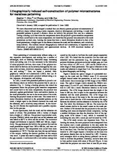
found in references such as ref.[42]. Based on this work, Choueiri[43] derived expressions to obtain the temperature from pressure and density. As shown in Fig.(2.1), it is clear that at temperatures at or above 104 K, the deviations from the ideal gas model are significant. This relation for the equation of state will be used in the current model, and further details
Figure 2.1: Deviation from ideal gas behavior for Argon
29
can be found in the appendix. As energy is deposited into the internal modes, the ratio of specific heats also changes. Once again, this can be calculated from the data of partition functions. As seen in Fig.(2.2), the deviation from the ideal value of
5=3 is severe at temperatures above 104 K, which is
consistent with Fig.(2.1).
Figure 2.2: Variation of the ratio of specific heats for argon (calculated from data in ref.[42])
2.3.6 Anomalous Transport It is known that the current can drive microinstabilities in the thruster plasma which may, through induced microturbulence, substantially increase dissipation and adversely impact
30
the efficiency. The presence of microinstabilities in such accelerator plasmas has been established experimentally in the plasma of the MPDT at both low and high power levels[44], [45]. Choueiri[16] has developed a model to estimate the resulting anomalous transport and heating in terms of macroscopic parameters. Under this formulation, apart from the classical collision frequency of the particles, there exists additional momentum and energy transferring collisions between particles and waves. The resulting anomalous collision frequency is important whenever the ratio of electron drift velocity to ion thermal velocity, s
j ude Mi = vti ene 2kB Th
� 1:5 :
(2.37)
Above this threshold, the ratio of anomalous collision frequency to classical collision frequency was found to depend on the classical electron Hall parameter, e , and the ratio of ion to electron temperatures, Th =Te . Polynomials giving these relations were derived in ref.[16] to be, �e;AN �e;cl
=
f0:192 + 3:33 � 10 2 e + 0:212 2e + TT f1:23 � 10 3 1:58 � 10 2 e h e
8:27 � 10 5 3e g
7:89 � 10 3 3e g ;
and are shown in Fig.(2.3). As a result, the effective resistivity of the plasma is now,
�eff =
me (�e;cl + �e;AN ) : e2 ne
(2.38)
2.3.7 Ionization Processes It is imperative that, within the acceleration region, a significant fraction of the working fluid remains in a state of ionization, as the free charges are responsible for carrying current, and thereby establishing the electromagnetic fields required for acceleration. The reaction rates for ionization reactions must account for transitions from the ground states, as well as 31
Figure 2.3: Ratio of anomalous to classical resistivity in argon plasmas (from ref.[16])
those from excited states. The work at the University of Stuttgart[46] has indicated that, for the conditions of interest to MPD plasmas, the solution of flow fields using the seemingly restrictive assumption of equilibrium ionization model may sufficiently be close to reality. In equilibrium, irrespective of the manner in which the species are created, the densities of the electrons, ne , ions, ni , and the neutrals , no , are related by the Saha[47] equation, i ni ne 2 (2�me kB T )3=2 l gl e = P i 1 ni 1 h3 l gl e P
�il =kB T �il 1 =kB T
= Ki ;
(2.39)
where �il is the lth energy level of the species of ionization level i, and gli is the corresponding statistical weight. Similar expressions can be written for higher ionization levels, with the energy levels scaled to a common ground. The propellant considered in this work is argon, and its first, second and third ionization potentials are 15.755 eV, 27.63 eV, and 40.90 eV respectively. The relevant energy levels of argon atom and its ions, and their statistical weights are given 32
in Table (2.1). Even in the presence of thermal nonequilibrium between electrons and ions, a modified Saha equation can be applicable. As shown in refs.[48] and [49], in such situations, due to the high mobility of the electrons, the temperature in eqn.(2.39) can be replaced with the temperature of the electron fluid, and the resulting modified Saha equation is an accurate model. Table 2.1: Energy levels and statistical weights in argon and argon ions (obtained from refs. [50], [51] and [52]) Ar I
Ar II
Ar III
Ar IV
g0l
E+ l (eV)
g+ l
E++ l (eV)
g++ l
E+++ (eV) l
g+++ l
0.000
1
0.059
6
0.111
29
0.000
4
11.577
8
13.476
2
1.737
6
3.478
16
11.802
4
16.420
20
4.124
2
14.671
24
13.096
24
16.702
12
14.214
6
31.133
24
13.319
12
17.177
6
17.856
1
35.568
40
14.019
48
17.688
28
17.964
10
14.242
24
18.016
6
19.460
14
14.509
24
18.300
12
20.066
1
14.690
12
18.438
10
20.222
8
E0l (eV)
For a model with N levels of ionization, the electron number density can be obtained by finding the single positive root of the polynomial (from Heiermann[37]),
nNe +1
+
N
X
l=1
"
nNe l (ne 33
lno )
l
Y
m=1
#
Km = 0 ;
(2.40)
where no is the total number density of all nuclei, and the equilibrium constant, Km is from eqn.(2.39).
2.3.8 Summary of Governing Equations The nucleus of this model is the set of single fluid MHD equations. The corresponding conservation laws, given by eqns. (2.8), (2.10), (2.12) and (2.24), can be summarized in the vector form:
2
@ @t
6 6 6 6 6 6 6 6 6 6 4
� �u
B E
3
2
7 7 7 7 7 7 7 7 7 7 5
6 6 6 6 6 6 6 6 6 6 4
+r�
�u
�uu + p� B��M
uB Bu (E + p) u B��M � u
3
2
7 7 7 7 7 7 7 7 7 7 5
6 6 6 6 6 6 6 6 6 6 4
=r�
0 ��vis E� res
q
3 7 7 7 7 7 7 7 7 7 7 5
:
(2.41)
Under this framework, ancillary relations such as the energy equation for the individual species, which do not fit into the conservation form, are solved separately, without affecting the underlying solver. Notice that the equations strictly contain a
r � B term, that is not
included in the conservation form. This will be discussed in the subsequent section.
2.3.9 Zero Divergence Constraint Though it is physically true that r � B
� 0, it is often not true numerically, as there may
be truncation errors. The treatment of the terms are important, since they could be a cause of numerical instabilities, as explained in ref.[53]. The technique used here, based on the work of Powell[54], has a modified eigensystem (cf. appendix xB.1) that accounts for any possible errors in r � B. The resulting scheme satisfies the relation,
@ (r � B) + r � [(r � B) u] = 0 : @t
(2.42)
In other words, the numerical scheme used in this work ensures that any artificial source of
r � B is convected out of the domain. 34
In the case of a self-field accelerator in a coaxial geometry, the magnetic field is purely azimuthal. If the assumption of axisymmetry is made, then � r � B = 1r @B =0: @�
(2.43)
Therefore, in this work, the divergence of the magnetic field is always zero throughout the domain.
2.4 Summary In summary, the physical models and the corresponding governing equations that describe MPDT flows were discussed in this chapter. The set of MHD equations, comprising the conservation relations for mass, momentum, energy and magnetic flux were described. Further improvements to the MHD model, such as the effects of thermal nonequilibrium, anomalous transport effects, along with relations for classical transport, a real equation of state and a multi-level equilibrium ionization model, were also developed in this chapter. The techniques for obtaining a numerical solution of these governing equations will be discussed in the following chapter.
35
Chapter 3 NUMERICAL SOLUTION Where the mind is without fear, and the head is held high . . . Rabindranath Tagore Despite several earlier efforts in the front of MPDT flow simulation, as mentioned in
x1.2, there remains a need for accurate and robust numerical schemes for this purpose. A new numerical method that has the potential to overcome the problems described in x1.2, will be described in this chapter. First, some fundamental concepts, pertaining to the guiding principles to be used in this thesis, will be reviewed. Then, the characteristics-splitting technique for the solution of the convection equations will be developed and validated. That will be followed by a brief discussion of the well known techniques for the solution of the diffusion equations.
3.1 Guiding Principles In light of the discussion in x1.2, it is imperative that the numerical scheme developed in this work to strictly adhere to the guidelines listed below: 1. Treat the flow and magnetic field equations in a self-consistent manner, 36
2. Use a conservative formulation of the problem, 3. Use non-oscillatory discontinuity capturing techniques that satisfy Rankine-Hugoniot relations, combined with techniques to limit numerical diffusion and improve spatial accuracy. The mathematical foundation for the numerical solver used in this work will be described in this chapter.
3.2 Mesh System The fundamental aspect of a numerical solution obtained through differencing schemes, unlike that of an analytical solution, is that it is defined on a discrete domain. A rigorous treatment of this issue can be found in ref.[55], and only the information directly relevant to the present application will be discussed here. The true domain, D , is divided into small control volumes, j , whose centers are given by position vectors cj . Within each of these
control volumes, the solution U(x; t) is approximated by a constant Uj (t), which should be considered as an approximation of the mean value of U over the cell i rather than the value of U at point cj ,
Uj (t) �= j 1 j
where j i j is the volume of i .
i
Z
i
U (x; t) d3 x;
(3.1)
Given an initial distribution U(x; 0), and using the definition in eqn.(3.1), the time rate
of change of U inside the control volume can be calculated from the sum of the fluxes through its boundaries,
@ Uj (t) = @t
1 XZ j ij
ij
where ij is the boundary between cells i and j . 37
F � ni dA;
(3.2)
Figure 3.1: Uniform, orthogonal structured grid. The adjoining issue is the detailed description of the control volumes, their identities, shapes, sizes, and locations. Mesh generation is an entire field of study in itself, and is beyond the scope of this work to get into the intricacies of that trade. Only a brief review that is relevant to the problem at hand will be made. Generally, cylindrical coordinates are preferable for the study of plasma thrusters. Three distinct techniques of dissecting the domain into control volumes can be identified: 1. Structured, concentric cylindrical shells, separated by lines of constant r^,
�^ and z^.
Combined with the axisymmetric assumption, the control volumes are simply rectangles in the r
z plane (cf. Fig.(3.1)).
2. Structured shells, separated by lines of a constant stream functions,
�; � that fit the
true boundaries as close as possible. Combined with the axisymmetric assumption, the control volumes are quadrilaterals in the r
z plane (cf. Fig.(3.2)).
3. Unstructured irregular tetrahedrons that fit the true boundary exactly. Combined with the axisymmetric assumption, the control volumes are triangles in the r Fig.(3.3)).
38
z plane (cf.
Figure 3.2: Non-uniform, structured grid (obtained from ref.[26]).
Figure 3.3: Non-uniform, unstructured grid. 39
Grids of type 3 may seem very attractive because of their adaptability to complex geometries, and have been popular (cf. refs.[23, 24]). However there are some disadvantages that may not be immediately apparent. Unstructured grids are computationally expensive and there are problems in extending higher order accurate schemes to them. Since the precise control of geometry may not be as critical to the design of plasma thrusters as it is to, say aircraft design, the use of unstructured grids may not be as worthwhile. This work currently uses grids of type 1. Though they are computationally inexpensive and easy to implement, they has been found to be too restrictive on the types of real thrusters that can be simulated. Therefore, work is underway, beyond what is reported in this thesis, to implement this solver on body-fitted grids of type 2. It is important to note that the numerical schemes, that will be developed in this chapter, will not require any fundamental changes to be applied on grids of type 2. The variables to be computed, given by U in eqn.(3.1), can be stored either in the vertices of the cells, or in the center of the cells (further discussion can be found in ref.[56]). In the former, the variables will coincide with the boundary, and they will be specified as boundary conditions. In the latter, the faces of the cells will be aligned with the walls, and the fluxes of these variables will be specified as boundary conditions. While solving the conservative formulation, it is preferable to choose the cell-centered scheme since specifying the fluxes is more compatible with the governing equations.
3.3 Consistency, Stability, and Convergence The true mathematical form of the systems of conservation laws are integral relations, while the partial differential forms are actually a special case, in which smoothness of the solution is assumed. To use the differential form in the presence of a discontinuity in the solution, one has to introduce the concept of weak form of the differential equations (cf. 40
LeVeque[40]). Often, there are more than one possible weak solutions, of which, of course, only one is physical. If the numerical scheme converges to a solution, the question to be answered is, “Is it the correct solution?”.
3.3.1 Lax-Wendroff Theorem The above question is answered by the Lax-Wendroff theorem, that states that (cf. [40]): If the numerical approximation computed with a consistent and conservative method converges, then the converged solution is the correct solution of the conservation law. Notice that though the Lax-Wendroff theorem is a powerful result, it does not help to determine if a scheme is convergent, but merely assures that the converged solution is the correct one.
3.3.2 Criteria for Stability and Convergence For a linear numerical scheme there are a few techniques available to analyze stability. The most popular of these was developed by John von Neumann[57] during the Manhattan project and is commonly referred to as the von Neumann stability analysis (VNSA). It involves discrete Fourier transforming the solution and inspecting the growth of waves in the frequency space. This approach is intuitively obvious because, like many physical instabilities, numerical instabilities are often a result of unbounded growth of certain oscillations. Using this technique, it is possible to decide on physically allowable combinations of grid spaces and time steps, that can result in a stable numerical scheme. Given a consistent and stable linear numerical scheme, the goal is to ensure that, as the discrete grid is refined to better emulate the continuous domain of the true solution,
41
the discrete solution approaches the true solution. In other words, the solution should converge. These three concepts, consistency, stability and convergence, are related by the Lax Equivalence Theorem which assures that (cf. [40]): For a properly posed initial value problem, with a consistent linear numerical scheme, stability is the necessary and sufficient condition for convergence. This is indeed a useful result, since the VNSA can determine the stability of a linear method, and consistency can be easily verified, it is straightforward to determine if the numerical solution will converge to the true solution. However, nonlinear convergence and stability are not simple extensions of their analog in the linear system. The Lax equivalence theorem is strictly applicable only to linear numerical schemes. Though some nonlinear equations can be linearized to obtained approximate answers, it is not of much help for truly nonlinear set of equations. For problems, such as the set of conservation laws seen in eqn.(2.41), requiring nonlinear operators, the need for establishing convergence still exists. Compounding the difficulty is the fact that VNSA is of practical use only for linear equations. In the complex set of highly nonlinear equations, such as MHD equations and Euler equations of compressible gas dynamics, a discrete Fourier transform would yield different frequencies. However, without the principle of linear superposition, any sort of VNSA becomes intractable, as explained by Laney[58]. Over the years, research in numerical techniques has led to the development of techniques to determine the stability and convergence of nonlinear systems of equations. The most useful among these are discussed below.
42
Total Variation Diminishing Schemes One method of analyzing stability stems from the classical concept of total variation in real and functional analysis (cf. ref.[59]). Harten[60] adapted this to the sorts of functions seen in computational gasdynamics. The total variation of a function U can be defined as:
T V (U) =
Z
1 dU dx: 1 dx
(3.3)
For the discrete situation, 3.3 can be written as:
T V (Un ) =
X
j
Unj+1 Unj
:
(3.4)
It can be proven (cf. ref.[58]) that the solutions to the conservation equations must be total variation diminishing (TVD) in the sense:
TV
�
�
Un+1 � T V (Un) ;
(3.5)
for all time levels. Since oscillations add to the total variation, the TVD condition cannot be satisfied by unbounded growth of oscillations. Thus, the TVD condition can be used as a stability check for nonlinear equations.
Local Extremum Diminishing Schemes Though the TVD principle is a popular check for convergence, it has its limitations. Since it imposes a condition only on the global variations, a scheme satisfying TVD condition eqn.(3.5) could, theoretically, allow spurious local oscillations (cf. ref.[58]). A more practical limitation of the TVD condition is that its extension to multidimensional problems does not provide a satisfactory measure of oscillations. To overcome both these shortcomings, Jameson[61] has developed the concept of local extremum diminishing (LED) schemes, which is summarized below.
43
Any time dependent conservation law, such as eqn.(2.41), can be written in a general form:
dUj X = C (U dt j =6 k j;k k
Uj ) :
(3.6)
If the numerical scheme has a compact stencil, in which the value at the point is directly dependent only on its nearest neighbors, and if the coefficients are all non-negative, then: 8 > >
> :
If Uj is a local maximum, then, a local minimum, then, (Uk
� 0; k = j � 1;
(3.7)
= 0; else
(Uk
Uj ) � 0, causing ddtU � 0. Conversely, if Uj is Uj ) � 0, causing ddtU � 0. These schemes are, therefore, j
j
aptly called local extremum diminishing (LED). Apart from ensuring that there are no local oscillations, the schemes built on this condition can be easily extended to multi dimensions. It can be shown that TVD is actually a 1-D special case of the LED concept. It can be shown[61] that schemes built on obtaining information from the upwind part of a characteristic do satisfy positivity constraints (eqn.(3.7)) and are thus stable. This concept is used in the developing the numerical scheme used in this work.
3.4 Conservation Form From a numerical solution perspective, it can be shown that the conservative formulation is necessary to accurately capture discontinuities. This can be seen even in a simple equation such as the Burger’s equation (cf. ref.[40]):
@u @ (u2 =2) + =0 @t @x
(3.8)
If eqn.(3.8) is solved using non-conservative schemes such as Lax-Friedrichs,
unj +1
unj+1 + unj = 2
1
"
unj+1 + unj 1 unj+1 unj �t 2 2�x 44
1
#
;
(3.9)
or backward differencing, "
unj +1 = unj
n n uj
�t uj
unj �x
1
#
;
(3.10)
it can be verified that both eqns. and give incorrect solutions of eqn.3.8. However, a conservative numerical formulation of eqn.(3.8),
unj +1 = unj
�t h n 2 (u ) 2�x j
i
(unj 1)2 ;
(3.11)
will give the correct answer. For further information on this issue, refer to LeVeque[40]. Most of the discussion on the numerical techniques has emphasized the hyperbolic nature of the convective part of the problem. This is because the goal of this work is to simulate problems in propulsion, consequently computing the flow is the most important part. Also, the convective problem is the harder one to solve numerically. The dissipative part of the problem, which is responsible for adding a parabolic nature to the governing equations, is relatively well understood. However, as explained in section 3.1, there is strong coupling between the hyperbolic and the parabolic part of the problem. This coupling raises important issues in spatial as well as temporal discretization. The issue regarding the time scales is discussed in x3.5.2. In the case of spatial discretization, the issue is that schemes that are good for parabolic equations are not suited for hyperbolic equations. Consider a simple scalar diffusion equation,
@u @2u = � 2: @t @x
(3.12)
A standard scheme to solve this equation is the explicit central differencing scheme:
unj +1
=
unj + �t
"
unj+1
2unj + unj �x2
1
#
:
(3.13)
However, it can be easily verified that for a simple scalar convection equation,
@u @u + V = 0; @t @x 45
(3.14)
the FTCS scheme, eqn.(3.13), does not satisfy the positivity condition (eqn.(3.7)) and even fails the VNSA. On the other hand, a good scheme for solving the scalar convection equation is the explicit backward differencing scheme:
unj +1 = unj
�t � V
"
unj
unj �x
1
#
:
(3.15)
Obviously, this scheme will not work for the diffusion equation because the numerical domain of dependence does not contain the physical domain of dependence (recall the CFL condition). Therefore, it is clear that discretization of the convective and dissipative parts of the problem must be treated separately.
3.5 Hyperbolic (Convection) Equations 3.5.1 Spatial Discretization The numerical solution to the set of hyperbolic equations (eqn.2.41 without the diffusion terms) is based on techniques that are extensively used in computational fluid dynamics. Based on the pioneering work of Godunov[62], [63], the principles underlying the design of non-oscillatory discretization schemes for compressible flows have been well established. There are two important issues in the design of discretization schemes:
�
Estimating the numerical flux through cell boundaries, accounting for waves (discussed in appendix xB.1) traveling at different speeds, and possibly in different directions.
�
Obtaining non-oscillatory solutions and capturing discontinuities with sufficient accuracy. 46
The scheme used in this thesis is developed in terms of local extremum diminishing (LED) principle of Jameson[61]. The method can be explained using eqn.(2.41) in one spatial dimension,
dUj Hzj +1=2 Hzj + dt �z
1=2
= 0;
(3.16)
where,U is the vector of conserved variables, and Hz is the approximation of flux in the z^ direction. The true flux, obtained from eqn.(2.41), in the z^ direction can be split as,
Fz(U) = Fz(U)+ + Fz(U)
;
(3.17)
where the eigenvalues of dFz+ =dU are all non-negative, and the eigenvalues of dFz
=dU
are all non-positive. Then, the approximation of flux is estimated as,
Hzj+
1 2
= Fz+j + Fzj +1 :
Using eqn.(3.17), this can be rewritten as,
Hzj+
1 2
1 = (Fzj + Fzj +1 ) 2
Dzj+
1 2
;
where
Dzj+
1 2
=
1 hn + Fzj+1 2
Fz+j
o
There still remains a question of how Fz+ and
n
Fzj+1 Fzj
Fz
oi
:
(3.18)
can be evaluated. This evaluation is
possible if there is a matrix A, such that �
�
�Fzj +1=2 = A � �Uj +1=2 ; where �Fzj +1=2 points
= Fzj +1
(3.19)
Fzj , and �Uj+1=2 = Uj+1 Uj . Note that, in the case the
j + 1 and j are on opposite sides of a discontinuity, eqn.(3.19) indicates that this
scheme satisfies the Rankine-Hugoniot jump conditions exactly. 47
Since the ideal MHD equations are hyperbolic, they have real characteristics. Therefore, the characteristic directions or characteristic manifolds have important physical meaning, since all information propagates along them (as explained in refs. [64, 65]). Moreover, the eigenvectors of the Jacobian, A, are orthogonal and can be normalized. Therefore, the Jacobian can be diagonalized as:
A � R�R
1;
(3.20)
where R contains the right eigenvectors of A as its columns, and eigenvectors of A as its rows.
R
1 contains the left
� is the diagonal matrix of eigenvalues of A. Since � can be
easily split into,
� = �+ + �
;
A� � R��R
1
using eqn.(3.20), A can be split as,
:
(3.21)
Thus if there exists an A such that eqn.(3.19) is true, then, �
�
�Fz�j +1=2 = A� � �Uj +1=2 : Defining jAj = A+
A
(3.22)
, eqn.(3.18) can be written as,
Dzj+
1 2
=
1 jAj � �Uj+ 12 : 2
(3.23)
For the Euler equations, the matrix A was derived by Roe[66, 67]. However, this is not necessarily applicable to MHD equations. There have been efforts by Cargo[68] to derive such matrices for MHD equations. The literature[69] suggests that various forms of averaged matrices work satisfactorily. From Godunov’s theorem, it is evident that the scheme can only be first-order accurate, if it is to capture discontinuities. However, away from the discontinuities, the spatial accuracy of the scheme can be improved by including flux-limited anti-diffusion, Lz, described 48
by Jameson[61]:
Dzj+
1 2
=
1 h jAj �Uj+ 12 2
�
Lz �Uj+
3 2
; �Uj
�i
1 2
:
(3.24)
Essentially, this reduces numerical diffusion where it is not required. Similar equations can be written for the corresponding terms in the r^ direction. An alternative to characteristics-splitting for solving conservation form of the equations is to use artificial viscosity (scalar diffusion). In this formalism, the equivalent expression for eqn.(3.23) is,
Dzj+
1 2
=
1 j�j �Uj+ 12 : 2 max
(3.25)
Because of its low computational cost, scalar diffusion schemes such as eqn.(3.25) have been successfully adapted for industrial applications such as aircraft design. However, since these schemes tend to artificially smooth out the solution [61], eqn.(3.25) was only used in this work for comparison with eqn.(3.23).
3.5.2 Temporal Discretization Unlike in fluid mechanics, the equations of MHD allow many different types of waves to exist. Even though physically the flow velocity is the sought quantity of most interest to propulsion, numerically the velocity of the fastest wave is what determines the time-step constraints. In plasmas of propulsion interest, the fluid velocity is quasineutral plasma with charge density of
O(10
1 ) Torr and magnetic pressure of
O(104) m/s .
For a
O(1021)=m3 and thermodynamic pressures of
O(101) Torr, the fast magnetosonic wave speed is
typically of the same order of magnitude as the flow velocity. This indicates that an explicit time marching scheme is suitable. From the CFL criterion, the time step for such a problem would be O (10 8
10 9) s.
49
A multi-stage scheme can be chosen to march forward in time. Writing eqn.(2.41) as,
dU + F (U) = 0 ; dt
(3.26)
where F (U) represents the sum of all the fluxes, the multi-stage scheme can be written as:
U1 U2 U3 U4 Un+1
= Un
�1 �t F (Un ) ;
= Un
�3 �t F (U2 ) ;
= Un
�2 �t F (U1 ) ;
= Un
�4 �t F (U3 ) ;
= U4 :
The coefficients used in this work are �1
(3.27)
= 0:1084; �2 = 0:2602; �3 = 0:5052; �4 = 1:0,
and were obtained from ref.[70].
3.5.3 Verification Unsteady Case Riemann problem The test problem chosen to validate this scheme was of the classical Riemann problem type, which consists of a single jump discontinuity in an otherwise smooth initial conditions. In 1-D the problem is:
U (x; 0) =
8 > > < > > :
UL UR
if x < L2 if x �
L 2
:
(3.28)
The Riemann problem was chosen because it is one of the very few that have an analytical solution. This problem provides an excellent illustration of the wave nature of the equations. The solution to the Riemann problem is useful to verify the capturing of both smooth waves (characteristics) as well as non-smooth waves (shocks).
50
Figure 3.4: Comparison of calculated profiles of pressure and magnetic field, with exact solution The initial states used were very similar to the Sod’s problem[71] for Euler equations. They were:
Left :
8 > > > > > > > > > > > > > > > > > > > > > > > > > > < > > > > > > > > > > > > > > > > > > > > > > > > > > :
�
= 1:0
Vx = 0:0 Vy = 0:0 Vz = 0:0 Bx =
3 4
Right :
By = 1:0 Bz = 0:0 p
= 1:0
8 > > > > > > > > > > > > > > > > > > > > > > > > > > < > > > > > > > > > > > > > > > > > > > > > > > > > > :
�
=
1 8
Vx = 0:0 Vy = 0:0 Vz = 0:0 Bx =
3 4
:
(3.29)
By = 1:0 Bz = 0:0 p
=
1 10
Some sample results are shown in Fig.(3.5.3). In these figures, the fast rarefaction (FR) wave can be seen on the far right and the far left, as it is the fastest of the waves present in the problem. The slow shock (SS) and the compound wave (SM) have speeds less than that of the FR wave. 51
Steady-State Case Taylor state In order to simulate steady-state MHD flows, this solver can be used to solve the unsteady equations and marched to steady state. An important question is whether the solution remains in that steady state. To answer this question, a test problem was chosen, whose equilibrium solution is known analytically. This equilibrium solution is given as the initial condition for the solver. After marching several hundreds or thousands of time steps, a check is performed if the variables have changed from the initial conditions. The test problem chosen for this simulation was the Taylor State configuration[72]. Under certain conditions, described in ref.[72], when a bounded plasma is allowed to evolve, it will move quickly and dissipate energy before coming to rest. This stable equilibrium configuration can be analytically found using the minimum energy principle, and is of the form:
r � B = �B;
(3.30)
where � is an eigenvalue. Since the current is parallel to the magnetic field, the
j � B body force is identically
zero. Furthermore, if there are no thermodynamic pressure gradients, the plasma is in a state of force-free equilibrium. For an axisymmetric geometry, the resulting magnetic field profile is:
B� = B0 J1 (�r); Bz = B0 J0 (�r);
(3.31)
where Bo is a constant amplitude, J0 and J1 are Bessel functions of the first kind, of orders
0 and 1 respectively. For a Cartesian grid of dimensions Lx � Lz , with symmetry along the y^ direction, the magnetic field distribution satisfying eqn.(3.30) is:
52
Figure 3.5: Magnetic field in the Taylor state configuration
Bx = pB02 sin By =
�
�
�
m�x cos n�z Lx Lz � � � � n�z ; B0 sin m�x sin Lx Lz
Bz = pB02 cos
�
m�x Lx
�
sin
�
n�z Lz
�
; (3.32)
�
;
where m and n are eigenvalues. With these initial conditions, the code was run for 10000 time steps on a 100 � 100 grid. At the end, the solution had deviated from equilibrium by less than 0.5%. The results from the code for Bx given in eqn.(3.32) are compared with the exact solution in Fig.(3.5).
53
3.6 Parabolic (Diffusion) Equations 3.6.1 Spatial Discretization Numerical methods for parabolic equations are relatively commonplace. The parabolic terms can be written as, 2
Sdis = r �
6 6 6 6 6 6 6 6 6 6 4
0 ��vis E� res
q
3 7 7 7 7 7 7 7 7 7 7 5
;
where
r � T� vis = r � [�visru] ;
(3.33)
represents the loss of momentum due to viscous forces,
r � E� res =
r�
"
�� � (r � B) ; �o #
(3.34)
represents the resistive diffusion of the magnetic flux, including the Hall effect, and, "
r � q = r � f��vis � ug
(
E0 � B �o
)
#
o + k�th � rT ; n
(3.35)
represents the energy sources/sinks due to viscous heating, Ohmic heating, and thermal conduction respectively. Thus, the equations dictate that the numerical scheme should be second-order accurate in space. In the framework used here, this implies that the first derivatives of variables are to be known across cell faces. Therefore, a simple central-differencing scheme will be sufficient for this problem.
54
3.6.2 Temporal Discretization Physical dissipation brings in different characteristic time scales into the problem. They are: Viscous diffusion: Magnetic diffusion: Heat conduction:
� 10 = �o �r 2 =� � 10 = ne kB �r 2 =�th � 10
= ��r 2 =�visc
9s 10 9
10 10
11 s 11 s.
Since these time scales could reach the extremities of the ranges mentioned, the choice of the time stepping scheme can be made on a case-by-case basis. If these were vastly different, that would call for an implicit treatment of time stepping. If they are not vastly different, and an explicit fractional time-stepping scheme can be chosen.
Fractional Time Stepping In the situations when the time scales are less than two orders of magnitude apart, it may not be worthwhile to choose an implicit scheme, however a standard explicit or multi-stage time-stepping scheme would be prohibitively expensive because it would require evaluating the convective fluxes at the time scales of dissipative fluxes. In order to find an optimum, a fractional time-stepping scheme can be chosen. In this method, the equation,
@U + r � Fconv = r � Fdiff ; @t is marched forward at the dissipative time scale,
Fdiff.
(3.36)
�td , dictated by the dissipative fluxes,
Fconv, are evaluated only after N dissipative time steps. The number N is chosen such that the effective convective time step, �tc = N � �td , However the convective fluxes,
is still smaller then the convective time step dictated by the CFL condition. By reducing the time consuming operation of evaluation of the convective fluxes, the effective speed of the
55
computation increases significantly. This is the current choice of temporal discretization currently used in this work.
Implicit Treatment Depending upon the particular case being simulated, the convective and dissipative time scales could be far more disparate. In this situation, the reasonable choice would be to use an implicit time-stepping scheme. In such a situation, some standard method, such as Alternating Direction Implicit (ADI) (cf. ref. [64]) can be used to solve the diffusion equations, with the convective fluxes assumed to be a constant during that time scale. However, if this solver is to be implemented on a parallel computer, an ADI scheme will interfere will the effectiveness of the parallel computation process. Therefore, the pros and cons of this approach have to be investigated.
3.7 Summary The fundamental concepts of stability and convergence of a numerical solution were reviewed in light of the techniques used in this work. The concept of local extremum diminishing (LED) schemes was introduced, and a new characteristics-splitting scheme, with flux-limited anti-diffusion to improve spatial accuracy was developed for the solution of the ideal MHD equations. This scheme was validated against unsteady (Riemann problem) and force-free equilibrium (Taylor state) test cases, and has demonstrated the ability the capture discontinuities monotonically, and good spatial accuracy in smooth regions of the solution. In conjunction with standard techniques for the numerical solution of parabolic equations, these schemes will be applied to simulate plasma flows in a real MPDT configuration in the following chapter.
56
Chapter 4 MPD THRUSTER SIMULATIONS “Has anything escaped me? I trust that there is nothing of consequence which I have overlooked?” Dr.Watson to Sherlock Holmes The Hound of the Baskervilles
In this chapter, the numerical techniques described in chapter 3 will be applied to solve the governing equations of the physical model developed in chapter 2, to simulate plasma flows in a gas-fed, self-field MPDT with a constant area channel. The geometry of the thruster, and the relevant initial and boundary conditions for obtaining a solution are described in this chapter. The resulting profiles for many plasma parameters, obtained from the calculations, are compared with experimental data for the given operating conditions, but on a somewhat different geometry.
4.1 Application of Governing Equations The conservation form of the MHD equations, given in eqn.(2.41), describe the evolution of eight variables, namely the total density (�), three components of momentum (�u; �v; �w ), three components of magnetic field (Br ; B� ; Bz ), and the total energy (E ). However, in a 57
self-field MPDT the magnetic field is purely azimuthal. Moreover, due to the assumption of axisymmetry, azimuthal momentum can be neglected. Though the solver described in
x3.1 - x3.6 is for the generalized set of eight equations, it can be reduced for a system of five equations: the total density (�), two components of momentum (�u; �w ), one component of magnetic field (B� ), and the total energy (E ). Expanding the vector-tensor form of eqn.(2.41) in cylindrical coordinates, using the identities eqns. (A.5), (A.6), and (A.7), along with the assumptions stated above, the MHD equations are: 2
@ @t
6 6 6 6 6 6 6 6 6 6 6 6 6 6 4
� �u �w B�
E
3
2
7 7 7 7 7 7 7 7 7 7 7 7 7 7 5
6 6 6 6 6 6 6 6 6 6 6 6 6 6 4
@ = @r
�u �
3
2
7 7 7 2 7 7 o 7 7 7 7 7 7 7 7 7 � 5 2
6 6 6 6 6 6 6 6 6 6 6 6 6 6 4
�u2 + p + 2B� �uw Ez0
qr
u
uB�
�
�
E + p + 2B�
@ + @z
o
3
�w �uw �
7 7 7 7 7 7 � 7 2 7 7 o 7 7 7 7 7 � 5 2
�w2 + p + 2B�
+ Sr (4.1)
(Er0 + wB� )
qz
w
�
E + p + 2B�
o
with 2
Sr = 1r
6 6 6 6 6 6 6 6 6 6 6 6 6 6 4
3
�u �
�u2 + B�o
2
�uw 0
qr
u
�
�
7 7 7 7 7 7 7 7 7 7 7 7 7 7 � 5 2
E + p + 2B�
qr = qz =
Ez0 B� @Th @Te �o + kth;e @r + kth;i @r � � � � Er0 B� @Te + k @Th + k th;e @z th;i @z �o �
�
�
�
o
These equations are solved, in combination with species energy equations (eqn.(2.30) and/or eqn.(2.31)), at every time level, throughout a specified domain (to be described in
x4.2), for a given set of initial and boundary conditions, to be described in x4.4 and x4.3 respectively. 58
4.2 Geometry The geometry chosen for this simulation was one of the series of constant area coaxial thrusters, shown in Fig.(4.1), used by Villani[31]. The primary reason for the choice of this thruster was that its simple geometry was more amenable to the structured orthogonal grid generation routine that is currently being used. The computational domain is shown in Fig.(4.2). Due to the assumption of axisymmetry, only one half of the cross section, starting from the centerline (surface #1), had to be included in the simulation. In this particular case, the cathode and the anode radii were 0.95 cm and 5.10 cm respectively. The cathode and the anode lengths were 26.4 cm and 20.0 cm respectively. Because of the inadequacy of the grid generation routine, the hemispherical tip of the cathode was represented as a flat tip (surface #8) in the simulation. For the same reason, the anode in the simulation has a sharp corner (interface of surfaces #4 and #5), instead of the rounded corner of the actual anode. The location of propellant injection ports in the real thruster are shown in Fig.(4.1). Due to the complexity of the physical processes near the inlet region in MPDTs (to be discussed in x), the simulation has an ionized propellant entering the domain uniformly (surface #6). The real thruster would operate either in the unbounded vacuum of space or in a bounded vacuum of a test chamber. However, the computational domain has to be restricted to something much smaller in size (surfaces #2 and #3). In this case, it is truncated at one cathode length downstream of the tip of the cathode (52.8 cm). Issues in this truncation are discussed in x4.3.
59
Figure 4.1: Geometry of the thruster chosen for simulation (lc = 26.4 cm)
Figure 4.2: Schematic of the computational domain (not to scale)
60
4.3 Boundary Conditions The set of governing equations (4.1) describe the evolution of many types of drastically different plasma flows. It is the role of the boundary conditions to distinguish one problem from another. For the particular MPDT simulation at hand, there are eight boundaries in the computational domain (cf. Fig.(4.2)), and they are of various types. This section will discuss the estimation of the convective and dissipative terms at each type of boundary.
4.3.1 Flow Properties Freestream The computational domain is assumed to be large enough such that there are no normal gradients in any of the flow properties at the free stream boundaries (surfaces #2 and #3). Solid Walls In reality, a sheath is formed at the interface of the plasma and the solid boundaries (surfaces #4, #5, #7, and #8). However, the sheath is a non-quasineutral region, and the fluid theory is not applicable there. Moreover, the size of the sheath region is typically of the order of a few Debye lengths, making it too small to be resolved by conventional grids. Therefore sheaths are currently ignored in this simulation. Discussion on inclusion of this effect will be made in x5. At solid boundaries, all convective fluxes into the wall, given in eqn.(2.41), are zero. If viscous effects were included, they would require that the tangential component of velocity to be zero at the wall. However, diffusive fluxes are nonzero. To calculate thermal conduction into a wall, the equations require that either the temperature of the wall, or the net heat flux to the wall itself, be specified. Ideally, the simulation would self-consistently and continuously compute the heat transfer from the plasma to the wall, then the heat transfer within the metallic 61
conductor, then calculate the temperature distribution of the wall, and from that information recompute the heat transfer from the plasma to the wall. Clearly, these calculations are computationally expensive, and may be impractical. However, there isn’t sufficient data to make good estimates of either of those quantities. Unlike the Li-LFA (described in
x1.2, and in ref.[9]), high-power, inert gas, self-field MPDTs are generally operated in a quasi-steady mode, in which the pulse length are � 2ms. The heat capacity of the plasma is typically not high enough to raise the temperature of the electrodes significantly in that duration, and there have been no known reliable measurements of heat transfer. In reality, there may be a thermal boundary layer in which the temperature varies from a few hundred Kelvin to more than an eV in a very small distance. Such sharp gradients may not be resolvable in simulations. Therefore a judicious estimate for heat transfer or wall temperature has to be made. The results in x4.7 were obtained with the temperature of the wall fixed at 2500 K. Centerline At the axis of symmetry (surface #1), there are no radial convective fluxes. Moreover, there are no radial gradients. Therefore, there is no thermal conduction across the centerline. Inlet At the inlet (surface #6), a specified mass flow rate of the propellant enters at a specified temperature at sonic conditions. In reality, the propellant is injected as neutral gas at room temperature, and it gets almost fully ionized within a few millimeters from the inlet[51]. However, it is believed[73] that this ionization process cannot be modeled by fluid theory. Therefore, in this model, the inlet temperature is chosen to be high enough such that the propellant is sufficiently ionized. Effectively, the backplate of the numerical model is not the true backplate, but a region few millimeters downstream of it.
62
4.3.2 Field Properties Freestream The computational domain is chosen to be large enough such that all the current is enclosed within the domain. Thus, from Amp`ere’s law, the magnetic field at the free stream boundaries (surfaces #2 and #3) is zero. Note that if the domain is too small making this assumption unreasonable, the simulation will yield unphysical results. For instance, the gasdynamic pressure is obtained by subtracting the contributions of magnetic field energy and kinetic energy from the total energy (refer to x2.3.4). If the magnetic field is sharply reduced to zero at the freestream boundaries, then there will be a corresponding unphysical increase in the gasdynamic pressure. Therefore, the domain has to be large enough to make this assumption reasonable. Solid Walls At all other boundaries, the magnetic field is computed purely from Faraday’s law. Using Stokes’ theorem it can be written as,
@B � dA = A @t
Z
I
C
E � dl :
(4.2)
In the cell-centered scheme used in this work, eqn.(4.2) implies that the evolution of the magnetic flux is specified by the contour integral of electric field around the cell. Therefore, the only information required is the electric field drop along the boundaries. From classical electromagnetic theory[74], the jump in the magnetic field,
H 2 H1 ,
across an interface between two media has to satisfy the relation,
n^ � (H2 H1) = Js ;
(4.3)
where Js is the surface current per unit length. Due to the no mass flux condition, the potential drop at a wall (surfaces #4, #5, #7, and #8) is entirely resistive, and is given by,
Ew = �w jw : 63
(4.4)
At conducting boundaries (surfaces #4, #5, #7, and #8), all the current entering the discharge flows at the surface, at least in the transient case. Therefore, even though resistivity,
�w , for most conductors is very small compared to the plasma resistivity, �plasma �copper �tungsten
� O (10 3 = 1:7 � 10 = 5:6 � 10
10 4 ) Ohm.m ; 8 Ohm.m ;
(4.5)
8 Ohm.m ;
the surface electric field is significant, due to the large current density in the transient case. In a true steady state, after the magnetic field has diffused into the conductor, the surface potential drop decreases to zero. At insulated boundaries, the magnetic field diffuses into the wall instantaneously. Therefore, the jump in the the magnetic field, and subsequently the surface current, is zero. Centerline At the axis of symmetry (surface #1), the inductive component of the electric field is zero because there is no flow across it. The resistive component can be related to the magnetic field from the point next to r
= 0, through a simple Taylor series expansion,
Ez0 jr=0 = �jz jr=0 = �
4 B� j�r=2 : �o �r
(4.6)
Inlet At the backplate, which also serves as the inlet (surface #6), the total voltage drop is set as the boundary condition. Emulating a true constant current circuit, this applied voltage is adjusted every time step to maintain the specified amount of current to flow in the channel.
4.4 Initial Conditions The governing equations (4.1) also require that the initial spatial distribution of the quantities be prescribed. The code is typically started with the entire domain filled with a back64
ground pressure of 10 4 Torr at a temperature of 300 K. Then, the inlet boundary conditions, corresponding to a fully ionized plasma entering at a specified mass flow rate, are imposed. After this plasma has filled the thrust chamber, the voltage at the backplate is made finite, introducing the effects of current and the magnetic field into the problem. For the calculations shown in x4.7, the current increased from 0 to 15 kA in �
5�s, and this rate is controlled by the adjustments to backplate voltage every
time step. Until this moment, the ionization is frozen to be Z=1, and the ratio of specific heats is fixed to be
= 5=3. After the current has permeated throughout the thrust chamber,
the effects of multi-level equilibrium ionization and non-ideal equation of state are slowly introduced. For instance, let � be the calculated value of at a time level n + 1, and n be the old value at time level n. Then, the value of used at time level n + 1 is:
n+1 = f� � g + f(1 �) n g ;
(4.7)
where � is a relaxation parameter between 0 and 1. A similar method is used for introducing ionization effects. This sort of “relaxation” is required to make the transition from an unphysical initial condition to a more realistic scenario.
4.5 Schematic of Calculations For a given set of initial and boundary conditions, the governing equations are solved using the techniques described in x3.1- x3.6. The entire process of simulation is illustrated in a flow chart in x4.5. The actual code, written in C/C++, is given in appendix xC. The input, consisting of the mass flow rate, the total current, the geometry, the grid sizes, and the total time are handled by the program “InputOutput.CPP” (xC.4). The grid itself is generated by the program “Grid.CPP” (xC.5). The initial values for all the rel65
Start Mass flow rate, J, Geometry, Grid size, Time
Generate Grid Initial Conditions Compute secondary variables and transport coefficients Set Boundary Conditions Estimate time step Compute fluxes Update conserved variables Convergence check Intermediate outputs t = t+deltaT
t >= Time ?
Final Output
End Figure 4.3: Schematic of the simulation process
66
evant variables are prescribed by the program “InitialConditions.CPP” (xC.6). The required secondary variables, and transport properties are computed in the program “RaCalculate.CPP” (xC.17). The boundary conditions are handled by “BoundaryConditions.CPP” (xC.7). The time steps is set by “SetTimeStep.CPP” (xC.9). The convective fluxes are computed in “EvalConv.CPP” (xC.10). The diffusive fluxes are computed in “EvalDiss.CPP”
(xC.14. The conservative variables are updated for the new time level in “TimeMarch.CPP”
(xC.15). At the same time, the species energies are computed in “Energy.CPP” (xC.16). At every time level, the convergence rates are calculated in the program “ReCalculate.CPP” (xC.17). The outputs are handled by “InputOutput.CPP”(xC.4).
4.6 Convergence and Stability Checks In order to verify convergence, there are two types of diagnostics in the code. In the first diagnostic, the change of conserved variables between every time level is calculated. In each case the largest change in the domain, and the average change over the entire domain are stored. Monitoring the maximum change helps check for stability. Monitoring the average change helps check for convergence. Since the entire set of equations is of the form,
dU +r�F =0; dt
(4.8)
monitoring �t � r � F is the appropriate measure of change in U. The time history of the average change throughout the domain is shown in Fig.(4.4). In the second diagnostic, the maximum value in the domain, and the average value over the domain of the conserved variables are stored. As before, monitoring the maximum value helps check for stability, and monitoring the average value helps check for convergence. The time history of the average value throughout the domain is shown in Fig.(4.4). From these plots, it was observed that convergence is reached only after � 67
2:0 � 106 time
Figure 4.4: A. Convergence rates for the conserved variables; B. Domain averaged values of i) Density, ii) Axial momentum, iii) Magnetic field, and iv) Total energy at each time step
68
steps, which corresponds to variables are shown in x4.7.
� 200�s of physical time.
The converged values of relevant
4.7 Results The results shown in this section are for the geometry in x4.2, with argon flowing in at 6.0 g/s and a discharge current of 15.0 kA. These conditions correspond to nominal operating conditions for the MPDT, since, from eqn.(2.7), �
' 1:0. There exists sufficient experimen-
tal data[31, 75] at these conditions, but for somewhat different geometries. The profiles of various relevant quantities are shown in this section.
4.7.1 Density The electron number densities within the chamber range from ' 1�1021 =m3 near the anode region, to ' 3 � 1021 =m3 near the cathode (see Fig.(4.5)). This increase may be attributed
to the radial pumping force, jz B� , which pushes the plasma away from the anode, towards the cathode. This trend has been observed in experiments and in previous simulations[19].
4.7.2 Ionization Levels The effective ionization fraction is calculated to be,
n Zeff = i=Ne ; X ni
(4.9)
i=0
where ne is the electron number density, and ni is the density of the ith ionized species. The resulting distribution is shown in Fig.(4.6). The presence of Ar-III and a small amount of Ar-IV in the plume is in agreement with experimental observations (cf. ref.[39]) for these 69
Figure 4.5: Distribution of electron number densities (in #/m3 )
Figure 4.6: Distribution of ionization levels
70
Figure 4.7: Distribution of electron temperatures (in eV)
operating conditions. From Fig.(4.6), it can be seen that the effective ionization fraction in the chamber is Zeff
' 1:0.
Since the model with frozen ionization (Zeff
� 1:0) has
been known to converge faster, one could use the single-level ionization model instead of the multi-level Saha model described in x2.3.7, to obtain rough estimates inside the thrust chamber.
4.7.3 Electron Temperatures The distribution of electron temperatures (in eV) is shown in Fig.(4.7). Within the thrust chamber, Te varies from about 1.0 to 1.5 eV. The lower values near the anode are probably due to the lower value of �j 2 at higher r, and large heat transfer to the walls. Nevertheless, these numbers are in general agreement with measurement[75] at these operating conditions. The hot spot at the tip of the anode, where Te is about 2.0 eV, is probably due to the strong current attachment in that region, causing augmented values of Ohmic heating (�j 2 ). The hot spot at the tip of the cathode may be due to stagnation, when the kinetic energy of the electron fluid is reduced and appears as thermal energy.
71
Figure 4.8: Distribution of ion temperatures (in eV)
4.7.4 Ion Temperatures The distribution of ion temperatures (in eV) is shown in Fig.(4.8). Within the thrust chamber, Th varies from about 1.0 to 1.5 eV. The hottest region of ion temperatures occurs at the axis of symmetry. At the center of the cathode tip (r=0), the ion temperature exceeds 4.0 eV. A partial explanation for this region of high temperature may once again be related to stagnation. Another possible explanation could be that the axisymmetric assumption causes thermal conduction at the centerline to go to zero. If there are symmetry breaking oscillations in reality, then there would be thermal conduction that would reduce the temperature in that region[76]. Nevertheless, these numbers are in general agreement with measurements[75] at these operating conditions.
4.7.5 Velocities The distribution of axial velocities in the domain are shown in Fig.(4.9). At the anode plane, the axial velocity ranges from 8.0 km/s to 15.0 km/s. The maximum velocity increases to a maximum of 17.0 km/s slightly further downstream. As expected, the velocity increases with decreasing radius, because of the similar trend in j � B. As mentioned in x2.2, the 72
Figure 4.9: Distribution of axial velocities (in m/s)
Figure 4.10: Velocity stream lines in the flow
thrust, consequently exhaust velocities, should be roughly independent of the geometry. As expected, these numbers from these simulations compare well with measurements of a different geometry in ref.[75]. To look at the effect of radial velocity on the flow, the velocity streamlines (where the velocity vector is a tangent at every point) are shown throughout the domain in Fig.(4.10).
4.7.6 Magnetic Field & Enclosed Current The spatial distribution of magnetic field strength in the domain is shown in Fig.(4.11), as a fraction of the maximum value. The maximum value attained, 0.26 T, is at the intersection 73
Figure 4.11: Distribution of magnetic field (as % of maximum)
Figure 4.12: Enclosed current contours (1500 A between lines)
of the backplate and the cathode. Generally,
B� varies as 1=r with radius and decreases
linearly with axial distance. This is strictly true for a uniform current distribution in the channel. However, the current and magnetic field propagate downstream via convection and diffusion, and their distributions are no longer uniform. The enclosed current is calculated as,
Jencl =
2�rB� : �o
(4.10)
The contours of enclosed current are shown in Fig.(4.12). Clearly, the current attachment is strongest near the backplate, and at the exit. This pattern is generally observed in many 74
Figure 4.13: Radial electric field contours (in Volts/m)
Figure 4.14: Axial electric field contours (in Volts/m)
MPDT geometries.
4.7.7 Electric Field & Potential By definition, the relationship between a static electric field and its potential is,
E (r; z) = r� (r; z) :
(4.11)
So, the potential difference between any two points can be calculated as,
� (r2 ) � (r1 ) = � (z2 ) � (z1 ) = 75
Z
r2
E � dr ; z E � dz : z
r
Z1
1
2
(4.12)
Figure 4.15: Potential contours (in Volts)
In this calculation, the cathode was set at a reference potential of 0. The potential at every other point in the domain was computed using eqn.(4.12). It is important to note that the predicted values of voltage do not include electrode drops, and are therefore cannot be compared to the measured value across the electrodes. Nevertheless, they do serve the purpose of quantifying the plasma part of the voltage drop. This simulation predicts a voltage drop across the plasma of 30.83 Volts. The true voltage drop is 56 Volts [31], and the difference can be attributed to the 25 Volts of anode drop that was measured.
4.7.8 Hall Parameter & Anomalous Transport The distribution of the electron Hall parameter in the domain is shown in Fig.(4.16). Within the channel, it varies from 0.3 to 1.2. Since the magnetic field and species temperatures increase with decreasing radius, so does the Hall parameter. Outside the channel, the Hall parameter is higher at the electrode tips than in any other region. Once again, referring to Fig.(4.11) and Fig.(4.7), the magnetic field is higher (cyclotron frequency is higher) and temperatures are higher (collision frequencies are lower) in those regions. It maybe worthwhile to note that these values of the electron Hall parameter are substantially lower than those observed in other MPDT configurations, such as the FSBT men76
Figure 4.16: Distribution of the Hall parameter tioned in x2.2. This is because, unlike in many MPDT configurations (e.g. ref.[75]) in which the anode is only a “lip” at the exit, the anode here is along the entire length of the channel, leading to a more diffuse current attachment pattern. Moreover, the propellant injection in this simulation is more uniform than in reality. This precludes regions of low densities and collisionality in the thrust chamber. As seen in Fig.(2.3), the ratio of anomalous resistivity to classical resistivity (eqn.2.38) is a strong function of the electron Hall parameter, beyond a cutoff, ude =vti
� 1:5.
The
ratio of anomalous resistivity to classical resistivity for this case is shown in Fig.(4.17). As expected for this value of J 2 =m _ , the Hall parameter is not very large in this particular case, and therefore the overall effect of anomalous transport is limited (cf. Fig.(2.3)).
4.7.9 Thrust & Efficiency By definition, the thrust is computed using the following relation,
T=
Z
A
uz (�u � dA) ;
where the integral is performed over all the boundaries in Fig.(4.2).
77
(4.13)
Figure 4.17: Ratio of anomalous to classical resistivity As discussed in x2.2, the analytical expression for thrust is, � �o � ra T= ln + A J 2 ; 4� rc
(4.14)
where ra and rc are the radii of the anode and the cathode respectively. For this particular case, the appropriate value for the current attachment parameter,
A, is 0.15 (refer to
Villani[31]). Notice that A is much smaller than ln rrac (which is 1.68). Using eqn.(4.13), the code predicts a thrust of 42.9 N. This compares well with the analytically calculated value is 41.2 N. By definition, the thrust efficiency is,
�th =
T2 2m_
VJ
;
(4.15)
where V is the total voltage drop, 30.83 Volts, and J is the total current, 15.0 kA. This yields a thrust efficiency of 33.2%. Clearly, this value is higher than the real thrust efficiency because voltage drops due to electrode falls are neglected. As mentioned earlier, the true voltage drop is 56 Volts, resulting in a thrust efficiency of 18.3%.
78
4.8 Summary Due to the limited capabilities of the grid generation routine used in this work, a simple constant area geometry was chosen for simulation. The drawback of this choice was the dearth of data available for this geometry. In fact, the only available data were the current and potential contours. The measured and calculated current contours are compared in Fig.(4.18). It is evident that in the simulation the current has not propagated as far downstream as in the experiment. A possible explanation is that the values of resistivity in the channel in the simulation, are higher than in reality. Though the computed values of electron temperatures are generally in the correct range, resistivity is a strong function of temperature (� Te 3=2 ), and without experimental data on the Te distribution, it is impossible to say if the resistivity values are correct. Increased values of Te , which will yield reduced values of
� will allow for the
current lines to propagate further downstream. This may be related to the unresolved issue of temperature boundary conditions, mentioned in x4.3.1. A direct comparison between measured and calculated potential contours cannot be made, because the calculations do not include electrode drops. Since the experimental measurements indicate that the anode drop is 25 V, the calculated potential contours were shifted by 25 V. Though this value is not a constant along the anode, it nevertheless allows comparison of calculations with measurements. These contours are shown in Fig.(4.19). It can be seen that the region in space that corresponds to the 30 V contour in the experiment, roughly corresponds to the 33 V contour in the simulation. Similarly, the region in space that corresponds to the 40 V contour in experiment, roughly corresponds to the 45 V contour in calculations. Again, it is important to bear in mind that the calculated contours were shifted by an estimate for anode drop. The unadjusted calculated contours are in Fig.(4.15).
79
0.102 0.092 0.082 0.071 0.061 0.051 0.041 0.031 0.020 0.010 0.000 0.000
2500
Anode 5000 12500
1000
7500
Cathode 0.026
0.053
0.079
0.106
0.132
0.158
0.185
0.211
0.238
0.264
0.290
0.317
0.343
0.370
0.396
0.422
0.449
Figure 4.18: Measured (top) and calculated (bottom) current contours
0.102 0.092 0.082 0.071 0.061 0.051 0.041 0.031 0.020 0.010 0.000 0.000
33
Anode
45
Cathode 0.026
0.053
0.079
0.106
0.132
0.158
0.185
0.211
0.238
0.264
0.290
0.317
0.343
0.370
0.396
0.422
Figure 4.19: Measured (top) and calculated (bottom) potential contours
80
0.449
As far as the other variables are concerned, the only comment that can be made is that their values and distributions are within a reasonable range of values observed in experiments on similar geometries for these operating conditions. Anomalous transport was found to have no major effect on the solution at these conditions. This is to be expected, since at this modest value of J 2 =m _ the electron Hall parameters are not very high for this geometry (cf. Fig.(2.3)). Though other researchers[24] have found the ideal equation of state suitable to simulate MPDTs at lower current levels, for the chosen operating condition, J
= 15.0kA, and
m_ = 6.0g/s, there were insufficient energy sinks with the ideal equation of state, and the simulation did not converge. A real equation of state was crucial to obtaining a realistic and stable solution. This chapter illustrated the application of the numerical techniques developed in this thesis to solve the governing equations of the physical model relevant to the simulation of plasma flows in a gas-fed, self-field MPDT functioning at nominal operating conditions. The calculated profiles for many relevant plasma parameters, and the calculated contours of current and electric potential, were compared with experimental data for the given operating conditions, but on somewhat different MPDT geometry. The calculated value of thrust was found to be in excellent agreement with the Maecker’s law (eqn.(2.6)).
81
Chapter 5 CONCLUDING REMARKS . . . I have promises to keep, And miles to go before I sleep, And miles to go before I sleep. Robert Frost
5.1 What are the contributions of this thesis? The objective of this thesis was to develop a numerical simulation model for MPD flows, that incorporates the state-of-the-art in numerical methods and physical models. For this purpose, a new numerical scheme to accurately compute plasma flows of interest to propulsion was developed and validated against standard test problems. The scheme treats the flow and the field in a self-consistent manner, and conserves mass, momentum, magnetic flux and energy. The characteristics-splitting scheme, which was developed from concepts used for the solution of Euler equations, was used to solve the ideal MHD equations. The ability of this scheme to capture discontinuities monotonically was demonstrated. Flux-limited anti-diffusion was used to improve spatial accuracy away from discontinuities. On top on the ideal MHD model, relevant diffusive effects, namely resistivity with Hall 82
effect and gradient drifts, and electron and ion thermal conduction were included. Furthermore, effects of thermal non-equilibrium between electrons and ions were incorporated. Anomalous transport effects, which account for momentum transfer between waves and particles in finite beta MPD flows, were included in the transport models. A real equation of state model, to account for energy deposition into internal modes, was included and was found to have significant effect on producing realistic and stable solutions. A multi-stage equilibrium ionization model was used to obtain ionization levels and species densities. This solver was then used to simulate a constant area coaxial MPDT, at nominal operating conditions corresponding to nominal operating conditions (�
' 1:0).
The resulting
profiles of densities, velocities, species temperatures, along with current and potential contours, when compared with existing data on MPDTs operating at this condition, but on somewhat different geometry, were found to be realistic. The value of thrust predicted by the simulation was in excellent agreement with predictions from analytical models. With that, the goal stated earlier has been attained. With the inclusion of anomalous transport effects and a real equation of state, the capabilities of the physical model exceed that of some of the most persistent efforts at other institutions to simulate MPD flows. There is no documentation of any existing code that was validated against standard MHD test cases. Furthermore, unlike any other existing MPDT flow simulation codes, this one uses modern numerical methods for the solution of the governing equations. Though this solver has demonstrated the ability to simulate MPD flows, it still requires development in both physical modeling and numerical capabilities. These are outlined in the subsequent section.
83
5.2 What remains to be done? 5.2.1 Computational Methods In order for this code to be a more practical tool for MPDT research, it requires improvements in the computational methods. First and foremost is the need to accelerate convergence, while maintaining temporal accuracy. Currently, with the explicit time-stepping scheme that is being used (though a sub-stepping scheme is sometimes applicable) it takes somewhere between many days to two weeks (on a Pentium-II 450MHz) for the solution to converge. Clearly, this hampers productivity and precludes the ability to test various cases. Therefore, the immediate next step in this work is to accelerate convergence by modifying the code to work efficiently on parallel computers. Though the time-step limiting diffusive fluxes can be treated implicitly, this will interfere will the effectiveness of the parallel computation process. The pros and cons of this approach have to be investigated. Perhaps the biggest limitation faced so far by the code is its structured orthogonal grid generation routine. This has precluded further validation of the code with existing experimental data, because of the limitations on the geometries that can be allowed by the simulation. Therefore, it is of utmost importance to develop a better grid generation routine. However, it is important to note that the numerical schemes developed in this thesis will not require any fundamental changes to be applied on grids of type 2 (Fig.(3.2)). Structured, curvilinear, body-fitted grids (Fig.(3.2)) are probably the best choice, and they will allow the code to simulate almost all known MPDT geometries. After the implementation of this grid generation routine, the code will be used to simulate the Princeton Configuration ’A’ thruster [75]. Since there is a plethora of data available on this geometry, it will serve as a good validation for the code.
84
5.2.2 Physical Models The list of possible improvements to the physical model can be extensive. Among these, a few are discussed in this section, as they are believed to be most significant to obtaining realistic and reliable simulations. In order to bolster its reliability, this code has to be used to simulate MPDTs operating at higher values of J 2 =m _ , for various geometries. In the case shown in x4.7, the effect of anomalous transport was limited because of the low values of electron Hall parameter. At higher values of J 2 =m _ , the effects of anomalous transport will be more pronounced. Some aspects of the physical models have been neglected so far, because their effects were assumed to be insignificant. First among these is viscosity. Given good physical models for the coefficient of viscosity, this effect can be added into the code without much difficulty. Another effect, which can be also added without any modifications, is ion-neutral slip. It was argued earlier, in x2.3.2 and x2.3.3, that these two effects were small. However, Niewood[19] attributes the high observed ion temperatures to viscous heating, and to ionneutral slip. Considering the ease with which these effects can be introduced, they will be incorporated soon into the code to test these propositions. While most of the boundary conditions, such as the no flux conditions, and electromagnetic jump conditions across interfaces, are self-explanatory, intuitively obvious, and are commonly used, others are not. As discussed in x4.3.1, the temperature boundary condition on the walls is not prescribed self consistently. The effect of changing the wall temperature, and/or modifying the heat flux condition has to be investigated thoroughly. Also, as discussed in x4.3.2, the size of the computational domain dictates whether the
B� = 0 condition at the freestream boundary is indeed realistic. It may be worthwhile to investigate the boundary condition on the centerline. As discussed in x4.7, in reality there may be some symmetry breaking oscillations at the centerline. Due to the axisymmetry
85
assumption used here, they are not accounted for. It is clear from the simulations that the species temperatures are high near this region. There may be a correlation between these two effects, which has to be investigated. As briefly mentioned in x4.3.1, there are two other issues that remain to be explored in the application of boundary conditions: sheaths, and inlet ionization. In reality, there exists a non-quasineutral sheath at the interface of a plasma and a solid boundary. For the plasma conditions of interest, the typical dimension of this quasineutral region, in which a large fraction of the voltage drop occurs, is �
O(10
5 )m. Clearly, this
cannot be self-consistently computed because: i) the physical processes in this region are beyond the regime of MHD theory, and ii) the dimensions are too small to be captured by grids. Therefore, the only way to include this effect is to superimpose a sheath model as a boundary condition. Though an attempt was made by Boie et al.[23], it was later discontinued. Ideally, this model will incorporate the effect of thermionic emission, and possible effects of magnetic field, on a high-voltage sheath in an unsteady plasma. As mentioned earlier, the propellant to a MPDT is injected as neutral gas at room temperature, and it gets almost fully ionized within a few millimeters from the inlet[51]. Choueiri and Okuda[73] have performed further investigations on anomalous ionization in MPDTs, and have shown that the most likely explanation is due to non-Maxwellian distribution of electron energies due to the effect of microinstabilities. It is believed that this ionization process cannot be modeled by fluid theory. This work currently employs a multi-stage equilibrium model. However, there is sufficient evidence[51, 20] that the equilibrium model is too simplistic. Niewood[19] used a finite-rate ionization model developed by Sheppard[20], and Caldo[15] has used another finite-rate ionization model. However, these finite-rate models do not predict higher levels of ionization, which have been observed experimentally [39, 51]. As mentioned earlier, it is important to allow for the presence of
86
Ar-III and other highly ionized argon species in the model. Thus, it is clear that there is still a lot of room to develop a good model to describe ionization processes in MPDTs, and implement them in this code. The MPDT research at Princeton is focussed on the Lithium Lorentz Force Accelerator (Li-LFA), a variant of the conventional MPDT. In order to model this thruster, a real equation of state model for lithium has to be developed and implemented. Due to the lack of megawatt level testing facilities, many MPDTs, including Li-LFA, are sometimes operated with an applied magnetic field, to increase their thrust efficiency. Though the solver was originally developed with all components of magnetic field, it was later trimmed down to have only the azimuthal component of the magnetic field, to simulate self-field MPDTs in coaxial geometry. Therefore, for simulating applied-field MPDTs the code has to be modified to handle the effects of applied magnetic fields. Since this code solves the governing equations in a time-dependent manner, in principle it can be extended to the simulation of pulsed plasma thrusters (PPT) as well. Without delving into the physical processes in PPTs, it is clear that the most important additions to the code for this purpose should be a finite-rate ionization model, and a model for circuit equation. It is possible that this code could also play a role in guiding MPDT research issues such as thermal modeling, near-cathode plasma characterization and electrode thermal management to understand erosion processes, propellant selection, active turbulence control, nearfield plume model as a source for far-field plume simulations that study the role of plasma interactions and contamination of spacecraft, and other contentious issues in overall design optimization. In conclusion, it is important to note that the numerical solution techniques and many of the physical models discussed in this thesis can be applied to simulate plasma flows in other
87
devices such as railguns[77], plasma flow switch ciruit breakers [78], Z-pinch devices for fusion[79] and the Variable Specific Impulse Magnetoplasma Rocket (VASIMR) [80, 81].
88
Bibliography [1] K.E. Tsiolkovsky. Exploration of the Universe with Reaction Machines. The Science Review, 5, 1903. English translation from the website of Tsiolkovsky State Museum of the History of Cosmonautics. [2] R.G. Jahn. Physics of Electric Propulsion. McGraw-Hill, 1968. [3] A. C. Ducati, G. M. Giannini, and E. Muehlberger. Experimental results in highspecific impulse thermo-ionic acceleration. AIAA J., 2(8):1452–1454, 1964. [4] G. P. Sutton. Rocket Propulsion Elements. John Wiley, 1992. [5] R. G. Jahn and E. Y. Choueiri. Electric propulsion. Academic Press Encyclopedia of Physical Science & Technology, 2000. [6] E. Y. Choueiri, A. J. Kelly, and R. G. Jahn. Mass savings domain of plasma propulsion for LEO to GEO transfer. J. Spacecraft & Rockets, 1993. [7] J. K. Ziemer. Performance Scaling of Gas-Fed Pulsed Plasma Thrusters. PhD thesis, Princeton U., 2000. [8] K. Toki and K. Kuriki. On-orbit demonstration of a pulsed self-field magnetoplasmadynamic thruster system. J. Prop. Power, 16(5):880–886, 2000. [9] V. Kim, V. Tikhonov, and S. Semenikhin. Fourth quarterly (final) report to NASAJPL: 100-150 kw lithium thruster research. Technical Report NASW-4851, 1997. [10] J. E. Polk. Mechanisms of Cathode Erosion in Plasma Thrusters. PhD thesis, Princeton U., 1995. [11] E. Y. Choueiri. Advanced Problems in Plasma Propulsion. Princeton U. Lecture Notes, 1998. [12] K. Toki I. Kimura and M. Tanaka. Current distribution on the electrodes of MPD arcjets. AIAA J., 20(7):889, 1982. [13] T.Ao and T. Fujiwara. Numerical and experimental study of an MPD thruster. IEPC84-08, 1984. 89
[14] T. Miyasaka and T. Fujiwara. Numerical prediction of onset phenomenon in a 2dimensional axisymmetric MPD thruster. AIAA-99-2432, 1999. [15] G. Caldo. Numerical simulation of MPD thruster flows with anomalous transport. Master’s thesis, Princeton University, 1994. [16] E.Y. Choueiri. Anomalous resistivity and heating in current-driven plasma thrusters. Phys. Plasmas, 6(5):2290, 1999. [17] M. LaPointe. Numerical simulation of geometric scale effects in cylindrical self-field MPD thrusters. NASA-CR-189224, 1992. [18] J.M.G. Chanty and M. Martinez-Sanchez. Two-dimensional numerical simulation of MPD flows. AIAA-87-1090, 1987. [19] E. H. Niewood. An Explanation for Anode Voltage Drops in an MPD. PhD thesis, MIT, 1993. [20] E. J. Sheppard. Ionization Nonequilibrium and Ignition in Self-Field Magnetoplasmadynamic Thrusters. PhD thesis, MIT, 1992. [21] P.J. Turchi, P.G. Mikellides, K.W. Hohman, R.J. Leiweke, I.G. Mikellides, C.S. Schmahl, N.F. Roderick, and R.E. Peterkin Jr. Progress in modeling plasma thrusters and related plasma flows. IEPC-95-159, 1995. [22] D.C. Lilekis and R.E. Peterkin Jr. Effects of azimuthal injection asymmetry of MPD thruster performance using the MACH3 code. IEPC-95-2677, 1995. [23] C. Boie, M. Auweter-Kurtz, H.J. Kaeppeler, and P.C. Sleziona. Application of adaptive numerical schemes for MPD thruster simulation. IEPC-97-115, 1997. [24] J. Heiermann, M. Auweter-Kurtz, J. J. Kaeppeler, A. Eberle, U. Iben, and P. C. Sleziona. Recent improvements of numerical methods for the simulation of MPD thruster flow on adaptive meshes. IEPC-99-169, 1999. [25] R. S. Myong. Theoretical and Computational Investigation of Nonlinear Waves in Magnetohydrodynamics. PhD thesis, U. Michigan, 1996. [26] M. Auweter-Kurtz et al. Numerical modeling of the flow discharge in MPD thrusters. J. Propulsion & Power, 1989. [27] R. J. Goldston and P. H. Rutherford. Introduction to Plasma Physics. Institute of Physics Publishing, 1995. [28] H. Maecker. Plasma jets in arcs in a process of self-induced magnetic compression. Z. Phys., 141(1):198–216, 1955.
90
[29] E.Y. Choueiri. The scaling of thrust in self-field MPD thrusters. J. Prop. Power, 14(5):744–753, 1998. [30] M. S. DiCapua. Energy Deposition in Parallel-Plate Plasma Accelerators. PhD thesis, Princeton U., 1971. [31] D. D. Villani. Energy Loss Mechanisms in a Magnetoplasmadynamic Arcjet. PhD thesis, Princeton U., 1982. [32] D.Q. King. Magnetoplasmadynamic Channel Flow for Design of Coaxial MPD Thrusters. PhD thesis, Princeton U., 1981. [33] M. Mitchner and C.H. Kruger. Partially Ionized Gases. Willy-Interscience, 1973. [34] M. J. Wolff. A High Performance Magnetoplasmadynamic Thruster. Master’s thesis, Princeton University, 1984. [35] D. J. Heimerdinger. Fluid Mechanics in a Magnetoplasmadynamic Thruster. PhD thesis, MIT, 1988. [36] Yu. P. Raizer. Gas Discharge Physics. Springer, 1997. [37] J. Heiermann, M.Auweter-Kurtz, and P.C. Sleziona. Adaptive computation of the current-carrying plasma in an MPD rocket thruster. Time-Dependent Magnetohydrodynamics: Anayltical, Numerical, and Application Aspects, 1998. [38] M. J. Boyle. Acceleration Processes in the Quasi-Steady Magnetoplasmadynamic Discharge. PhD thesis, Princeton U., 1974. [39] A. P. Bruckner. Spectroscopic Studies of the Exhaust Plume of a Quasi-Steady MPD Accelerator. PhD thesis, Princeton U., 1972. [40] R. J. LeVeque, D. Mihalas, E. A. Dorfi, and E. M¨uller. Computational Methods for Astrophysical Fluid Flow. Springer, 1998. [41] W. G. Vincenti and C.H. Kruger. Introduction to Physical Gas Dynamics. Kruger Publishing, 1965. [42] W. M. Sparks and D. Fischel. Partition Functions and Equations of State in Plasmas. NASA SP-3066, 1971. [43] E. Y. Choueiri. A Scaling Strategy for the Preliminary Design of MPD Thrusters. Master’s thesis, Syracuse University, 1983. [44] E.Y. Choueiri, A. J. Kelly, and R.G. Jahn. Current-driven plasma acceleration versus current-driven energy dissipation: Part ii: Electromagnetic wave stability theory and experiments. IEPC-91-100, 1991. 91
[45] D.L. Tilley, E.Y. Choueiri, A. J. Kelly, and R.G. Jahn. Microinstabilities in a 10kilowatt self-field magnetoplasmadynamic thruster. J.Prop.Power, 12(2):381, 1996. [46] H. O. Schrade, P. C. Sleziona, T. Wegmann, and H. L. Kurtz. Basic processes of plasma propulsion: Final report. AFOSR: 91-0118, 1991. [47] M. N. Saha. Ionization in the solar chromosphere. Phil. Mag., 40:472, 1920. [48] J. L. Kerrebrock and M. A. Hoffman. Nonequilibrium ionization due to electron heating. AIAA J., 2:1072, 1964. [49] S. Suckewer. Excitation and ionization of atoms and ions in a non-thermal plasma. II: Ionization equilibrium. J. Phys. B, 3:390–398, 1970. [50] J. Vlcek. A collisional-radiative model applicable to argon discharges over a wide range of conditions: Formulation and basic data. J. Phys.D, 22:623, 1988. [51] T. M. Randolph. Measurement if Ionization Levels in the Interelectrode Region of an MPD Thruster. Master’s thesis, Princeton University, 1994. [52] V. Kaufmann and W. Whaling. Improved wavelengths and energy levels of doublyionized argon ( ar iii). J. Res. Natl. Inst. Stand. Technol., 101:691, 1996. [53] J.U. Brackbill and D.C. Barnes. The effect of nonzero r� B on the numerical solution of the magnetohydrodynamic equations. J. Comp. Phys, 35:426, 1980. [54] K.G. Powell. An approximate Riemann solver for magnetohydrodynamics (that works in more than one dimension). NASA ICASE Report 94-24, 1994. [55] E. Godlewski and P. A. Raviart. Numerical Approximation of Hyperbolic Systems of Conservation Laws. Springer, 1996. [56] L. Martinelli. Calculations of Viscous Flows With a Multigrid Method. PhD thesis, Princeton U., 1987. [57] J. von Neumann. A method for the numerical calculation of hydrodynamic shocks. J. Appl. Phys., 21:232–237, 1950. [58] C. B. Laney. Computational Gasdynamics. Cambrigde, 1998. [59] H. L. Royden. Real Analysis. MacMillan, 1968. [60] A. Harten. High resolution schemes for hyperbolic conservation laws. J. Comp. Phys, 49:357–393, 1983. [61] A. Jameson. Analysis and design of numerical schemes for gas dynamics, 1: Artificial diffusion, upwind biasing, limiters and their effect on accuracy and multigrid convergence. Comp.Fluid.Dyn, 1995. 92
[62] S.K. Godunov. Finite difference method for numerical computation of discontinous solution of the equations of fluid dynamics. Matematicheskii Sbornik, 47:15–21, 1959. [63] S.K. Godunov. Symmetric form of the equations of magnetohydrodynamics. Numerical Methods for Mechanics of Continuum Medium, 1972. [64] S. C. Jardin. Computational Methods in Plasma Physics. Princeton U. Lecture Notes, 1998. [65] Jeffrey and Taniuti. Nonlinear Wave Propagation With Applications to Physics and Magnetohydrodynamics. Academic Press, 1964. [66] P. Roe. Approximate Riemann solvers, parameter vectors, and difference schemes. J. Comp. Phys, 43:357, 1981. [67] P. Roe. Characteristics-based schemes for the Euler equations. Annual Review of Fluid Mechanics, 18:337, 1986. [68] P. Cargo and G. Gallice. Roe matrices for ideal MHD and systematic construction of Roe matrices for systems of conservation laws. J. Comp. Phys, 136:446, 1997. [69] N. Aslan. Two-dimensional solutions of MHD equations with an adapted Roe method. Int. J. Num. Meth. in Fluids, 23(11):1211, 1996. [70] B. van Leer, C. H. Tai, and K. G. Powell. Design of optimally smoothing multi-stage schemes for the euler equations. AIAA-89-1933, 1989. [71] G.A Sod. A survey of finite-difference methods for systems of nonlinear conservation laws. J. Comp. Phys, 27:1, 1978. [72] J.B. Taylor. Relaxation of toroidal plasma and generation of reverse magnetic fields. Physical Review Letters, 1974. [73] E.Y. Choueiri and H. Okuda. Anomalous ionization in MPD thrusters. IEPC-93-067, 1993. [74] J.D. Jackson. Classical Electrodynamics. Wiley, 1975. [75] E. Y. Choueiri, A. J. Kelly, and R. G. Jahn. Pulsed electromagnetic acceleration: JPL contract no.954997. MAE Report, 1692.23, 1986. [76] R. G. Jahn, S. C. Jardin, and E. Y. Choueiri. Perosnal communication. Princeton University, 2000. [77] M. H. Frese. The internal structure and dynamics of the railgun plasma armature between infinitely wide ablating rails. Los Alamos Natl. Lab. Technical Report: LASUB-93-178, 1993. 93
[78] J. Buff, M. H. Frese, A. J. Giancola, R. E. Peterkin, and N. F. Roderick. Simulations of a plasma flow switch. IEEE Transactions on Plasma Science, PS-15:766–771, 1987. [79] U. Shumlak. A near-term, z-pinch fusion space thruster. AIAA-2000-3368, 2000. [80] F. R. Chang Diaz, J. P. Squire, R. D. Bengston, B. N. Breizman, F. W. Baity, and M. D. Carter. The physics and engineering of the VASIMR engine. AIAA-00-3756, 2000. [81] J. L. Cambier. Perosnal communication. MSE Technology Applications, Inc., 2000. [82] J.D. Huba. NRL Plasma Formulary. Naval Research Laboratory, 1994. [83] K.G. Powell et al. An upwind scheme for magnetohydrodynamics. AIAA-95-1704, 1995. [84] K.G. Powell et al. A solution-adaptive upwind scheme for ideal magnetohydrodynamics. J. Comp. Phys, 154:284–309, 1999.
94
Appendix A VECTOR OPERATIONS A.1 IDENTITIES The vector identities used in this chapter are available from the NRL Plasma Formulary[82]. In this notation, A, B, U are vectors, I� is the unit dyad and T� is a tensor.
(r � B) � B = (rB) � B (B � r) B
(A.1)
r � (AB) = (r � A) B + (A � r) B
(A.2)
B � B I� (rB) � B = r � 2
(A.3)
"
#
r � [u � B] = [u (r � B) + (B � r) u B (r � u) A 1 @A� @Az r r � A = @A + r+ + @r r r @� @z 95
(u � r) B]
(A.4)
(A.5)
2
r � T� = 2
rA =
6 6 6 6 6 6 4
6 6 6 6 6 6 4
1 @ r @r 1 @ r @r 1 @ r @r
@Ar @r � 1 @Ar r @� @Ar @z
(rTrr ) + (rTr� ) + (rTrz ) +
A�
�
@Tzr @z @Tz� @z @Tzz @z
+
T�� r T�r r
@A� @r � � 1 @A� + A r r @� @A� @z
3 7 7 7 7 7 7 5
@Az @r 1 @Az r @� @Az @z
(A.6)
3 7 7 7 7 7 7 5
(A.7)
A.2 MANIPULATIONS Using the definition,
�j = 1 hrB �o
i
rB y ;
and the Ohm’s law (without rpe drift) written in the form,
� B = �� � j ; E0 = �o j + j en e
(A.8)
the resistive diffusion of the magnetic field can be written as the divergence of the tensor, h i E� res = �� � �j
iy �� � �j
h
h
�o�j : i
In other words,
r � E0 = r � E� res :
96
(A.9)
Appendix B EIGENSYSTEM B.1 Eigensystem of MHD Alfv`en speeds:
CA;r;�;z = Bpr;�;z �o � , q
Sonic speed: a = p� Normalization coefficients (based on the work in refs.[83], [84])
p z;r;� = p
r;�;z =
CA;�;z CA2 ;� +CA2 ;z CA;r;� CA2 ;r +CA2 ;�
�r;f;s = �z;f;s =
r
� Ca C � Ca C
r
2 2 S;F ;r 2 2 F ;r CS ;r 2 2 S;F ;z 2 2 F ;z CS ;z
Fast and slow magnetosonic waves:
1 B�B 2 B � B + a2 )2 (4a2 C 2 ) = ( +a )� ( A; r 2 �o � �o � s " # 1 B�B 2 B � B 2 2 2 2 2 CF;S ; z = ( +a )� ( + a ) (4a CA; z ) 2 �o � �o � "
s
#
2 CF;S ;r
The Jacobian of transformation between primitive and conservation variables:
97
2
dU = dW
6 6 6 6 6 6 6 6 6 6 6 6 6 6 6 6 6 6 6 6 6 6 6 6 6 6 4
3
1
0
0
0
0
0
0
u
�
0
0
0
0
0
0
v
0
�
0
0
0
0
0
w
0
0
�
0
0
0
0
0
0
0
0
1
0
0
0
0
0
0
0
0
1
0
0
0
0
0
0
0
0
1
0
Bx �o
By �o
Bz �o
1
1
u�u
2
�u �v �w
7 7 7 7 7 7 7 7 7 7 7 7 7 7 7 7 7 7 7 7 7 7 7 7 7 7 5
B.1.1 rˆ Direction Eigenvalues (in non-decreasing order):
[u CF ;r ; u CA;r ; u CS ;r ; u; u; u + CS ;r ; u + CA;r ; u + CF ;r ]
(B.1)
Ortho-normalized eigenvectors i
h
�r;f CF ;r �r;s CS ;r r;� Sgn[Br ] �r;s CS ;r r;z Sgn[Br ] ; ; 0; �2arp;s �ro;�� ; �2arp;s �ro;�z ; 2��ar;f2 2a2 ; 2a2 2a2 h i L2r = 0; 0; pr;2z ; pr;2� ; 0; p 2r�;zo � ; p 2r�;�o � ; 0 i h L3r = 0; �r2;as2CS;r ; �r;f CF ;2r a2r;� Sgn[Br ] ; �r;f CF ;r2 a2r;z Sgn[Br ] ; 0; 2�arp;f� or�;� ; 2�arp;f� or�;z ; 2��ar;f2 h i L4r = 1; 0; 0; 0; 0; 0; 0; a21
L1r = 0;
L5r = [0; 0; 0; 0; 1; 0; 0; 0] h
L6r = 0; �r;2saC2S;r ; �r;f CF ;r2 ar2;� Sgn[Br ] ; �r;f CF ;r2 ar2;z Sgn[Br ] ; 0; h
i
L7r = 0; 0; pr;2z ; pr;2� ; 0; p 2r�;zo � ; p 2r�;�o � ; 0 h
L8r = 0; �r;2faC2F ;r ;
�rp;f r;� �rp;f r;z �r;f i 2a �o � ; 2a �o � ; 2�a2
�r;s CS ;r r;� Sgn[Br ] �r;s CS ;r r;z Sgn[Br ] ; ; 0; �2arp;s �ro;�� ; �2arp;s �ro;�z ; 2��ar;f2 2a2 2a2
98
i
p
h
R1r = ��r;f ; �r;f CF ;r ; �r;sCS ;r r;� Sgn [Br ] ; �r;sCS ;r r;z Sgn [Br ] ; 0; �r;sa r;� �o �; �r;sa r;z p�o �; �a2 �r;f
h
R2r = 0; 0; p r2;z ; pr;2� ; 0; h
i
r;pz p�o � r;�pp�o � i ; 2 ;0 2
p
R3r = ��r;s ; �r;sCS ;r ; �r;f CF ;r r;� Sgn[Br ]; �r;f CF ;r r;z Sgn[Br ]; 0; �r;f a r;� �o �; �r;f a r;z p�o �; �a2 �r;f
i
R4r = [1; 0; 0; 0; 0; 0; 0; 0] R5r = [0; 0; 0; 0; 1; 0; 0; 0]
R6r = ��r;s ; �r;sCS ;r ; �r;f CF ;r r;� Sgn[Br ]; �r;f CF ;r r;z Sgn[Br ]; 0; �r;f a r;� p�o �; h
�r;f a r;z p�o �; �a2 �r;f p
h
i
R7r = 0; 0; p r2;z ; pr;2� ; 0; r;zp2�o � ;
r;p� p�o � i ;0 2
R8r = ��r;f ; �r;f CF ;r ; �r;sCS ;r r;� Sgn[Br ]; �r;sCS ;r r;z Sgn[Br ]; 0; �r;sa r;� p�o �; h
�r;sa r;z p�o �; �a2 �r;f
i
B.1.2 zˆ Direction Eigenvalues (in non-decreasing order) �
w
CF ;z ; w
CA;z ; w
CS ;z ; w; w; w + CS ;z ; w + CA;z ; w + CF ;z
99
�
(B.2)
Ortho-normalized eigenvectors h
;rSgn[Bz ] �z;s CS ;z z;� Sgn[Bz ] L1z = 0; �z;sCS;z z ; ; 2a2 2a2 i
h
L2z = 0; p z2;� ; pz;2r ; 0; p2 �zo;�� ; p 2z�;ro � ; 0; 0 h
L3z = 0;
�z;f CF ;z �zp �z;f i ;s z ;r �z ;s z ;� p ; ; ; 0 ; 2a2 2a �o � 2a �o � 2�a2
i �z;f CF ;z z ;rSgn[Bz ] �z;f CF ;z z;� Sgn[Bz ] �z;s CS ;z �zp;f z;r �zp;f z ;� �z;s ; ; ; ; ; 0 ; 2a2 2a2 2a2 2a �o � 2a �o � 2�a2
L4z = [0; 0; 0; 0; 0; 0; 1; 0] h
L5z = 1; 0; 0; 0; 0; 0; 0; a21
i
h
L6z = 0; �z;f CF ;z2 za2;rSgn[Bz ] ; �z;f CF ;z2 az2;� Sgn[Bz ] ; �z;2saC2S;z ; h
i
L7z = 0; p z2;� ; pz;2r ; 0; p 2z�;�o � ; p2 �zo;r� ; 0; 0 h
L8z = 0;
�z;f z;r �z;f z ;� �z;s 2ap�o � ; 2ap�o � ; 0; 2�a2
�z ;f �z;s CS ;z z ;rSgn[Bz ] �z;s CS ;z z;� Sgn[Bz ] �z;f CF ;z �zp ;� ; ; 2a2 ; 2a;s �zo;�r ; �2az;ps z 2a2 2a2 �o � ; 0; 2�a2
i
i
p
h
R1z = ��z;f ; �z;sCS ;z z;r Sgn[Bz ]; �z;sCS ;z z;� Sgn[Bz ]; �z;f CF ;z ; �z;sa z;r �o �; �z;sa z;� p�o �; 0; �a2 �z;f
h
R2z = 0; p z2;� ; pz;2r ; 0;
i
i z;p� p�o � z;rpp�o � ; ; 0 ; 0 2 2
R3z = ��z;s; �z;f CF ;z z;r Sgn[Bz ]; �z;f CF ;z z;� Sgn[Bz ]; �z;sCS ;z ; �z;f a z;r p�o �; h
�z;f a z;� p�o �; 0; �a2 �z;s
i
R4z = [0; 0; 0; 0; 0; 0; 1; 0] R5z = [1; 0; 0; 0; 0; 0; 0; 0]
R6z = ��z;s; �z;f CF ;z z;r Sgn[Bz ]; �z;f CF ;z z;� Sgn[Bz ]; �z;sCS ;z ; �z;f a z;r p�o �; h
p
�z;f a z;� �o �; 0; �a2 �z;s h
p
R7z = 0; p z2;� ; pz;2r ; 0; z;�p2�o � ;
i
i z;pr p�o � ; 0 ; 0 2
R8z = ��z;f ; �z;sCS ;z z;r Sgn[Bz ]; �z;s CS ;z z;� Sgn[Bz ]; �z;f CF ;z ; �z;sa z;r p�o �; h
�z;sa z;� p�o �; 0; �a2 �z;f
i
100
Appendix C COMPUTER PROGRAM C.1 Main //---------------------------------------------------------//Thruster-Axi.CPP; Written by Kameshwaran Sankaran //---------------------------------------------------------#include "Thruster-Axi.h" #include #include #include #include #include #include #include #include #include #include #include
"InputOutput.cpp" "Grid.cpp" "Memory.cpp" "InitialConditions.cpp" "Solve.cpp" "SetTimeStep.cpp" "BoundaryConditions.cpp" "EvalConv.cpp" "EvalDiss.cpp" "TimeMarch.cpp" "ReCalculate.cpp"
void main() { GetInput(); MemAllocate(); SetInitial(); Solve(); }
101
C.2 Declarations //--------------------------------------------------------//Thruster-Axi.h; Written by Kameshwaran Sankaran //--------------------------------------------------------#include #include #include #include #include #include
FILE *ConvergeDiff, *ConvergeVal; FILE *Converge; const double PI=3.14159265359; const double Root2=1.4142136; //Acceleration due to gravity at Earth, in m/sˆ2 const double go=9.81; //Permeability of free space const double Mu=1.256637061436e-6; //Permittivity of free space const double Eps0=8.854187817e-12; //Ideal ratio of specific heats for Argon const double gamConst=1.666666666; //Boltzmann’s constant in Joules/Kelvin const double kBoltz=1.380658e-23; //Gas constant for Argon in J/Kg.K const double Rargon= 208.1333519883; //Mass of Argon ion in Kg const double mAr=6.63352599096e-26; //Mass of election in Kg const double mEl=9.1093897e-31; //Charage of electron in Coulombs const double q=1.60217733e-19; //1 electron volt in K //Resistivity of tungsten in Ohm.m const double eV=11604.44751705; const double ResTungst=5.6e-8; //Resistivity of copper in Ohm.m const double ResCopper=1.7e-8; //Thermal conductivity of tungsten in W/m.K const double ThermTungst=174.0; //Thermal conductivity of copper in W/m.K const double ThermCopper=401.0; int Ra, Rc, Za, Zc, numR=0, numZ=0, numT=0, row, col, i=0, j=0, k=0, l=0, m=0, J=0, K=0, numSteps=0, SubStep; int MaxStep=10; //These are variables for the equation of state. int In1, In2, In3, In4, In5, In2A, In2B, In3A, In3B, In4A, In4B; int Zone, Count; int ExtraMemory =0; double AnodeLength,CathodeLength,Ranode,Rcathode,MassFlowRate,Jmax; double RAD, Z, deltaR, deltaZ, TotTime, deltaT=1.0e-8, deltaTconv, deltaTtherm, deltaTresist, Lmax; double t = 0.0; double eps = 1.0e-15;//A small number, used to estimate cut offs. double Jback=0.0, Vappl = 10.0;//Initial guesses. //Guess for the temperature of the electrodes, in K. double ElecTemp = 3.0e3; double K0, K1, K2;//These are coefficients in the equation of state.
102
double RhoIn, VzIn, peIn, phIn, TeIn, ThIn; double Tinlet=0.0, Tupstream=0.0, Texit=0.0, Thrust=0.0, MaeckerT=0.0, Isp; int Rmin[4], Rmax[4], Zmin[4], Zmax[4];
//Vertices of the zone.
//These are scalars at every point. double **Vr, **Vz, **Cf, **SpecRadR, **SpecRadZ, **VSq, **aSq, **CmSq; double **Bt, **BSq; double **Er, **Ez, **ErH, **EzH, **EFr, **EFz, **jr, **jz, **jDens, **Jencl, **Potential; double **n, **Rho, **p, **E, **P; double **Res, **EIcollFreq, **ElecGyro, **ElecHall, **CoulombLog, **kTherm, **ElCondR, **ElCondZ, **kIon, **IonCondR, **IonCondZ, **ThermCondR, **ThermCondZ; double **Vde, **Vti, **AnomFreqEl, **TotCollFreq; double **PR, **gam, **gamOld;
//These are vectors at every point. double **u[5], **ConvFlux[5], **Hr[5], **Fr[5], **Dr[5], **SourceConv[5], **SourceR[5], **Lr[5], **Sr[5], **Hz[5], **Fz[5], **Dz[5], **Lz[5], **Sz[5], **DissFlux[5], **DissipR[5], **SourceDiss[5], **DissipZ[5]; //These are from "EvalD()". double **RdelU[5], **ZdelU[5]; //Variables for the two-temperature model. double **EintEl, **EintH, **ne, **neOld, **ni, **nii, **niii, **nA, **pe, **ph, **Te, **Th, **Zeff, **Qei, **Qeii, **Qeiii, **nuei, **nueii, **nueiii, **CGvosQ, **Ce, **FrEn, **FzEn, **DrEn, **DzEn, **SrEn, **ElecComp, **Ohmic, **Exchange, **EnFluxR, **EnFluxZ, **EnSourceR; //Convergence checks double **uOld[5]; double u0Dmax=0.0, u1Dmax=0.0, u2Dmax=0.0, u3Dmax=0.0, u4Dmax=0.0, u0Davg=0.0, u1Davg=0.0, u2Davg=0.0, u3Davg=0.0, u4Davg=0.0, u0DMaxR, u0DMaxZ, u1DMaxR, u1DMaxZ, u2DMaxR, u2DMaxZ, u3DMaxR, u3DMaxZ, u4DMaxR, u4DMaxZ, u0Max=0.0, u1Max=0.0, u2Max=0.0, u3Max=0.0, u4Max=0.0, u0Avg=0.0, u1Avg=0.0, u2Avg=0.0, u3Avg=0.0, u4Avg=0.0, u0MaxR, u0MaxZ, u1MaxR, u1MaxZ, u2MaxR, u2MaxZ, u3MaxR, u3MaxZ, u4MaxR, u4MaxZ; double double
**KEold, **KE, **Etherm, **EthOld; DensD=0.0, KED=0.0, BtD=0.0, EtotD=0.0, EthD=0.0, DensDavg=0.0, KEDavg=0.0, BtDavg=0.0,EtotDavg=0.0, EthDavg=0.0, DensMaxR, DensMaxZ, KEmaxR, KEmaxZ, BtMaxR, BtMaxZ, EtotMaxR, EtotMaxZ, EthMaxR, EthMaxZ;
/* //These are required by CharSplit(). double **rho, **ur, **uz, **bt, **hOld, **BtAvg; double **alfF, **alfS, **betaT, **ZalfF, **ZalfS, **ZbetaT; double **L1, **L2, **L3, **L4, **L5, **L1m, **L2m, **L3m, **L4m, **L5m, **L1p, **L2p, **L3p, **L4p, **L5p, **ZL1, **ZL2, **ZL3, **ZL4, **ZL5, **ZL1m, **ZL2m, **ZL3m, **ZL4m, **ZL5m, **ZL1p, **ZL2p, **ZL3p, **ZL4p, **ZL5p; //These are vectors are every point. double **R1[5], **R2[5], **R3[5], **R4[5], **R5[5], **Left1[5], **Left2[5], **Left3[5], **Left4[5], **Left5[5],
103
**R1z[5], **R2z[5], **R3z[5], **R4z[5], **R5z[5], **Left1z[5], **Left2z[5], **Left3z[5], **Left4z[5], **Left5z[5]; //These are matrices at every point. double **Lplus[5][5], **Lminus[5][5], **LplusZ[5][5], **LminusZ[5][5]; double **Lambda[5][5], **LambdaZ[5][5], **AbsLambda[5][5], **AbsLambdaZ[5][5]; double **Aplus[5][5], **Aminus[5][5], **Bplus[5][5], **Bminus[5][5]; double **Rp[5][5], **Lp[5][5], **RpZ[5][5], **LpZ[5][5]; double **R[5][5], **Rinv[5][5], **RZ[5][5], **RinvZ[5][5]; double **M[5][5], **Minv[5][5], **AbsA[5][5], **AbsB[5][5]; double **temp[5][5]; */ //FUNCTION DECLARATIONS... double EvalSign(double x); void void void void void void void void void void void void void void void void void void void void void void void void void
ConvBound(); DissBound(); EquationOfState(); EvalConv(); EvalDiss(); EvalEnergy(); EvalF(); EvalGamma(); EvalLim(); EvalNumDiss(); EvalParam(); EvalS(); EvalTimeStep(); EvalVar(); GetInput(); Grid(); MemAllocate(); ReCalculate(); Saha(); SetInitial(); Solve(); TerminalChars(); TimeMarch(); Transport(); WriteFile();
//Memory functions double **AllocMatrix(int RowBegin,int RowEnd,int ColBegin,int ColEnd); /* void ArtVisc(); void CharSplit(); void AllocMemoryEXTRA(); void EvalLambdaR(int Zone); void EvalLambdaZ(int Zone); void EvalVectorsR(int Zone); void EvalVectorsZ(int Zone); void EvalA(int Zone); void AverageR(int Zone); void AverageZ(int Zone); void EvalM(int Zone); void EvalMinv(int Zone); void MulMatrix(double **MatA[5][5], double **MatB[5][5], double **MatC[5][5], int Zone); void AddMatrix(double **MatA[5][5], double **MatB[5][5], double **MatC[5][5], int Zone); void SubMatrix(double **MatA[5][5], double **MatB[5][5], double **MatC[5][5], int Zone); void MatTimesVec(double **MatA[5][5], double **VecB[5], double **VecC[5], int Zone); void AddVector(double **VecA[5], double **VecB[5], double **VecC[5], int Zone);
104
void SubVector(double **VecA[5], double **VecB[5], double **VecC[5], int Zone); */
105
C.3 Memory Allocations //--------------------------------------------------------//Memory.CPP; Written by Kameshwaran Sankaran //--------------------------------------------------------void MemAllocate() { //Allocating the scalars. //Conservation variables Rho =AllocMatrix(0, numR+1, 0, numZ+1); Vr =AllocMatrix(0, numR+1, 0, numZ+1); Vz =AllocMatrix(0, numR+1, 0, numZ+1); VSq =AllocMatrix(0, numR+1, 0, numZ+1); Bt =AllocMatrix(0, numR+1, 0, numZ+1); BSq =AllocMatrix(0, numR+1, 0, numZ+1); E =AllocMatrix(0, numR+1, 0, numZ+1); //Primitive variables n =AllocMatrix(0, numR+1, 0, numZ+1); p =AllocMatrix(0, numR+1, 0, numZ+1); P =AllocMatrix(0, numR+1, 0, numZ+1); Er =AllocMatrix(0, numR+1, 0, numZ+1); Ez =AllocMatrix(0, numR+1, 0, numZ+1); ErH =AllocMatrix(0, numR+1, 0, numZ+1); EzH =AllocMatrix(0, numR+1, 0, numZ+1); EFr =AllocMatrix(0, numR+1, 0, numZ+1); EFz =AllocMatrix(0, numR+1, 0, numZ+1); jr =AllocMatrix(0, numR+1, 0, numZ+1); jz =AllocMatrix(0, numR+1, 0, numZ+1); jDens =AllocMatrix(0, numR+1, 0, numZ+1); Jencl =AllocMatrix(0, numR+1, 0, numZ+1); Potential=AllocMatrix(0, numR+1, 0, numZ+1); //Variables from the two-temperature model. EintEl =AllocMatrix(0, numR+1, 0, numZ+1); EintH =AllocMatrix(0, numR+1, 0, numZ+1); ne =AllocMatrix(0, numR+1, 0, numZ+1); neOld =AllocMatrix(0, numR+1, 0, numZ+1); ni =AllocMatrix(0, numR+1, 0, numZ+1); nii =AllocMatrix(0, numR+1, 0, numZ+1); niii=AllocMatrix(0, numR+1, 0, numZ+1); nA =AllocMatrix(0, numR+1, 0, numZ+1); pe =AllocMatrix(0, numR+1, 0, numZ+1); ph =AllocMatrix(0, numR+1, 0, numZ+1); Te =AllocMatrix(0, numR+1, 0, numZ+1); Th =AllocMatrix(0, numR+1, 0, numZ+1); FrEn =AllocMatrix(0, numR+1, 0, numZ+1); FzEn =AllocMatrix(0, numR+1, 0, numZ+1); DrEn =AllocMatrix(0, numR+1, 0, numZ+1); DzEn =AllocMatrix(0, numR+1, 0, numZ+1); SrEn =AllocMatrix(0, numR+1, 0, numZ+1); ElecComp=AllocMatrix(0, numR+1, 0, numZ+1); Ohmic =AllocMatrix(0, numR+1, 0, numZ+1); Exchange=AllocMatrix(0, numR+1, 0, numZ+1); EnFluxR =AllocMatrix(0, numR+1, 0, numZ+1); EnFluxZ =AllocMatrix(0, numR+1, 0, numZ+1); EnSourceR =AllocMatrix(0, numR+1, 0, numZ+1); //Dissipation variables Res =AllocMatrix(0, numR+1, 0, numZ+1); EIcollFreq =AllocMatrix(0, numR+1, 0, numZ+1); AnomFreqEl =AllocMatrix(0, numR+1, 0, numZ+1); TotCollFreq =AllocMatrix(0, numR+1, 0, numZ+1); ElecGyro =AllocMatrix(0, numR+1, 0, numZ+1);
106
ElecHall =AllocMatrix(0, numR+1, 0, numZ+1); CoulombLog =AllocMatrix(0, numR+1, 0, numZ+1); kTherm =AllocMatrix(0, numR+1, 0, numZ+1); kIon =AllocMatrix(0, numR+1, 0, numZ+1); IonCondR =AllocMatrix(0, numR+1, 0, numZ+1); IonCondZ =AllocMatrix(0, numR+1, 0, numZ+1); ElCondR =AllocMatrix(0, numR+1, 0, numZ+1); ElCondZ =AllocMatrix(0, numR+1, 0, numZ+1); ThermCondR =AllocMatrix(0, numR+1, 0, numZ+1); ThermCondZ =AllocMatrix(0, numR+1, 0, numZ+1); //Transport Zeff = AllocMatrix(0, numR+1, 0, numZ+1); Qei = AllocMatrix(0, numR+1, 0, numZ+1); Qeii = AllocMatrix(0, numR+1, 0, numZ+1); Qeiii = AllocMatrix(0, numR+1, 0, numZ+1); nuei = AllocMatrix(0, numR+1, 0, numZ+1); nueii = AllocMatrix(0, numR+1, 0, numZ+1); nueiii = AllocMatrix(0, numR+1, 0, numZ+1); CGvosQ = AllocMatrix(0, numR+1, 0, numZ+1); Ce = AllocMatrix(0, numR+1, 0, numZ+1); //Speeds aSq =AllocMatrix(0, numR+1, 0, numZ+1); CmSq=AllocMatrix(0, numR+1, 0, numZ+1); Cf =AllocMatrix(0, numR+1, 0, numZ+1); SpecRadR =AllocMatrix(0, numR+1, 0, numZ+1); SpecRadZ =AllocMatrix(0, numR+1, 0, numZ+1); //For anomalous transport Vde =AllocMatrix(0, numR+1, 0, numZ+1); Vti =AllocMatrix(0, numR+1, 0, numZ+1); AnomFreqEl =AllocMatrix(0, numR+1, 0, numZ+1); //For the equation of state PR =AllocMatrix(0, numR+1, 0, numZ+1); gam =AllocMatrix(0, numR+1, 0, numZ+1); gamOld =AllocMatrix(0, numR+1, 0, numZ+1); //For convergence checks KEold = AllocMatrix(0, numR+1, 0, numZ+1); KE = AllocMatrix(0, numR+1, 0, numZ+1); Etherm = AllocMatrix(0, numR+1, 0, numZ+1); EthOld = AllocMatrix(0, numR+1, 0, numZ+1); //Allocating the vectors. for (i=0; i Jmax >> RAD >> Ranode >> Rcathode >> Z >> AnodeLength >> CathodeLength >> numR >> numZ >> TotTime ; Grid(); } //------------------------------------void WriteFile() { //Temporary output if(numSteps%1000 == 0) { ofstream OutTemp("OUT-Temp.DAT"); OutTemp