SIMULATION OF OVERLOAD CONTROL IN SIP SERVER NETWORKS Pavel O. Abaev (speaker) Yuliya V. Gaidamaka Telecommunication Systems Department Peoples’ Friendship University of Russia Miklukho-Maklaya str., 6, 117198, Moscow, Russia Email:
[email protected],
[email protected]
KEYWORDS Signalling network, SIP, hop-by-hop overload control, threshold, hysteretic load control. ABSTRACT In this study, we investigated a signalling load control mechanism for SIP server networks and developed a corresponding queuing model. The so-called hop-by-hop overload control, known from recent IETF drafts and RFCs, was considered and a similar buffer overload control scheme which was developed for the SS7 signalling link in ITU-T Recommendation Q.704, was proposed. The mechanism is based on hysteretic load control with thresholds for reducing potential oscillations between the control-on and control-off states under certain loading conditions. Adjustment of three types of thresholds – the overload onset threshold, the overload abatement threshold, and the overload discard threshold – makes possible the regulation of signalling traffic to meet blocking requirements. In this study, we built and analyzed the M |M |1 queue with bi-level hysteretic input load control. A numerical example illustrating the control mechanism that minimizes the return time from overloading states satisfying the throttling and mean control cycle time constraints is also presented. INTRODUCTION Threshold load control is a well-known and reliable tool for preventing SS7 signalling link congestion (ITU-T Recommendation Q.704, 1996). In this paper, it is shown that the same technique (Takshing and Yen, 1983; Takagi, 1985) is applicable to overload control problems in a SIP server signalling network, stated in recent IETF RFCs and drafts (RFC 3261, 2002; RFC 5390, 2008; RFC 6357, 2011; IETF draft SIP Overload Control, 2012; IETF draft SIP Rate Control, 2012) and still not solved. To that end, we analyzed carefully the overloading control mechanism for SIP servers defined in (RFC 3261, 2002). Some variations of the control mechanism studied in numerous documents and papers, e.g. in (ITU-T Recommendation Q.704, 1996; RFC 3261, 2002; RFC 5390, 2008; RFC 6357, 2011; IETF draft SIP Overload Proceedings 26th European Conference on Modelling and Simulation ©ECMS Klaus G. Troitzsch, Michael Möhring, Ulf Lotzmann (Editors) ISBN: 978-0-9564944-4-3 / ISBN: 978-0-9564944-5-0 (CD)
Alexander V. Pechinkin Rostislav V. Razumchik Sergey Ya. Shorgin Institute of Informatics Problems of RAS Vavilova, 44-1, 119333, Moscow, Russia Email:
[email protected],
[email protected],
[email protected]
Control, 2012; IETF draft SIP Rate Control, 2012; Ohta, 2009; Hilt and Widjaja, 2008; Shen et al., 2008; Montagna and Pignolo, 2008; Garroppo et al., 2009; Montagna and Pignolo, 2008; Homayouni et al., 2010; Abdelal and Matragi, 2010; Montagna and Pignolo, 2010; Garroppo et al., 2011). We investigated a two-stage server overload processing comprising overload detection and overload mitigation. The total number of messages in the buffer, i.e. buffer occupancy, was monitored to detect overloading. In order to mitigate or eliminate overloading, we restricted or prohibited input signalling load. Three types of thresholds are used to control overloading – overload onset threshold H, overload abatement threshold L, and overload discard threshold R. Overloading occurs when buffer occupancy increases and exceeds the overload onset threshold, H. The input load is then reduced to avoid overloading. However, the load does not return to the normal load value immediately after overloading mitigation, but the buffer occupancy becomes lower than the overload abatement threshold, L, after decreasing. This technique is called hysteretic load control (ITU-T Recommendation Q.704, 1996) by analogy with the terminology of SS7. Two hysteretic thresholds (onset and abatement) are needed to reduce the potential oscillations between the control-on and control-off states under certain loading conditions. The paper is organized as follows. First, it is shown that overload can be implemented locally, hop-by-hop, and end-to-end according to (RFC 6357, 2011). Queuing models for local overload control have been proposed in (Abaev et al., 2011) and a queuing model for hopby-hop overload control is built in this study. Second, a queuing system with bi-level hysteretic load control is studied and an analytical solution for steady-state distribution of queue length and mean control cycle time derived. A numerical example is then presented and in conclusion, the main results of the study are summarized. DEVELOPING SIMULATION MODEL FOR SIP SERVER OVERLOAD CONTROL In this section, a simulation model for hop-by-hop overload control, which was proposed in (RFC 6357, 2011) is
built. Let us briefly describe the main features of the SIP mechanism, which is needed to convey overload feedback from the receiving to the sending SIP server. Three different alternative feedback mechanisms – local, hopby-hop, and end-to-end – are illustrated in Fig. 1, according to (RFC 6357, 2011). If overload control is implemented locally, the SIP server measures the current utility of its processor and makes a decision to select the messages that will be affected and determines whether they are rejected or redirected. In case of end-to-end overload control, all the receiving servers along the path of a request should measure the current utility of their processors and notify the sender of a request concerning overloading. All the receiving servers have to cooperate to jointly determine the overall feedback for this path. Each sending server implements the algorithms needed to limit the amount of traffic forwarded to the receiving server. Note that in (IETF draft SIP Overload Control, 2012), the local mechanism was recognized as ineffective and end-to-end mechanism deemed difficult to implement. Hop-by-hop overload control does not require that all SIP entities in a network support it. It can be used effectively between two adjacent SIP servers if both servers support overload control and does not depend on the support from any other server or user agent. The more SIP servers in a network support hop-by-hop overload control, the better protected the network is against occurrences of overload. Therefore, overload control is best performed hop-by-hop. The receiving SIP server monitors the current utility of its processor and notifies the sending server in case of overloading. The sending server acts on this feedback and reduces the outgoing load, for example, by rejecting messages if needed. According to the loss-based overload control mechanism (IETF draft SIP Overload Control, 2012), a server asks an upstream neighbour to reduce by the desired percentage the number of requests it would normally forward to this server. For example, a server can ask an upstream neighbour to reduce the number of requests by 10%. The upstream neighbour then redirects or rejects the messages that are destined for this server with dropping probability q = 0.1. The alternative is a rate-based overload control mechanism (IETF draft SIP Rate Control, 2012). When the rate-based overload control mechanism is used, a server notifies an upstream neighbour to send requests at a rate no greater than or equal to the desired number of requests per second. The above hop-by-hop overload control principles have been used as the basis of a simulation model and for formulation of the optimization problem of hop-byhop overload control. In addition, analytical formulae were developed to support the simulation. We considered the interaction between two adjacent SIP servers that use loss-based overload control mechanism and built a simple model with the aim of analyzing the control parameters using the bi-level hysteretic load control idea from (ITU-T Recommendation Q.704, 1996).
Similarly, the example discussed in (IETF draft SIP Rate Control, 2012), we are modeling message processing as a single work queue that contains incoming messages. Fig. 2 shows a single-server queuing system with hysteretic overload control with two thresholds, L and H. In the next section, this is denoted by M |M |1| hL, Hi |R according to the Kendall classification, where R stands for the overload discard threshold. Customers arrive at the system and receive service in accordance with the overload control algorithm. The mean processing time is µ−1 . The server operates in three modes: normal (s = 0), overload (s = 1), and discard (s = 2), where s is the overload status. When the queue length increases and exceeds the threshold, H, in the normal mode, the system detects the overload and switches to the overload mode. In the overload mode, the system reduces input flow: newly arriving customers are discarded with dropping probability, q. Thereafter, if the queue length decreases and drops below the threshold, L, in the overload mode, the system detects the elimination of overload, turns to normal mode and starts to put all newly arrived customers into the queue. If in the overload mode the queue length continues increasing and reaches threshold, R, the system turns to the discard mode and all newly arrived customers are discarded. After that, the queue length starts decreasing in the discard mode and when it drops below the threshold, H, the system detects mitigation of overloading, turns to the overload mode and starts to put newly arrived customers into the queue with probability p = 1 − q. Let n denote the queue length, n = 0, ..., R. Then the state space of the system is of the form X = X0 ∪X1 ∪X2 , where X0 is the set of states of normal load, X1 is the set of overload states, and X2 is the set of discard states. These sets are given by following formulae: X0 = {(s, n) : s = 0, 0 ≤ n ≤ H − 1} , X1 = {(s, n) : s = 1, L ≤ n ≤ R − 1} , X2 = {(s, n) : s = 2, H + 1 ≤ n ≤ R} . Then the input load function λ (s, n) is shown in Fig. 3 and specified by the following relation: (s, n) ∈ X0 , λ, λ (s, n) = pλ, (s, n) ∈ X1 , 0, (s, n) ∈ X2 . The probability of the system being in the set of normal load states is denoted by P (X0 ), the probability of being in the set of overload states by P (X1 ) , and the probability of being in the set of discard states by P (X2 ). Let τ0 denote the average duration of the system in set X0 . The key performance measures of the system are overload probability P (X1 ), discard probability P (X2 ), and τ as the mean return time from overloading states X1 ∪ X2 . Next, we analyze the model developed in this section, and derive formulas for the analysis of its key performance measures.
Domain 2
Domain 1
UA servers
UA сlients
. ..
. ..
Server 4
Server 3
Server 2 Server 1 Se
rve
r3
an d
Se
rve
Domain 3
r4
local hop-by-hop end-to-end Server 5
Figure 1: Types of overload control mechanisms
s, n
R
H L
Figure 2: M |M |1| hL, Hi |R queuing model QUEUING MODEL AND ITS PERFORMANCE MEASURES In this section, the queuing model with thresholds L, H, and R, shown in Fig. 2, and with input load function λ (s, n), shown in Fig. 3, is considered. The Markov process, X (t) = (s, n), which completely describes the system over the state space, X , is considered. Our goal is to find stationary probability distribution of the number of customers in the system, ps,n , (s, n) ∈ X , and the mean return time from the states of the set X1 ∪ X2 to the states of the set X0 , namely to the state (0, L − 1). To find the stationary distribution, some auxiliary variables were defined.
The probability that until the first time in the queue remain n + 1 customers, there will never be less than L customers is denoted by βn , n = L, . . . , H − 1. These probabilities can be calculated using the formula βL = λ1 /(λ1 +µ) and, according to the law of total probability, we have βn =
λ1 µ + βn−1 βn , n = L + 1, . . . , H − 1. λ1 + µ λ1 + µ
Equilibrium Equations It is easy to see that the stationary probabilities satisfy the following system of equilibrium equations: λp0,n−1 = µp0,n , n = 1, . . . , L − 1,
(µ + λ)p0,n = λαn+1 p0,n + λp0,n−1 , n = L, . . . , H − 2, (2) (µ + λ)p0,H−1 = λp0,H−2 , n = H − 1,
Auxiliary variables Let λ1 = pλ and denote αn , n = L, . . . , R − 1, n 6= H the probability that until the first time in the queue remains n−1 customers, there will never be R customers. Omitting the intermediate steps, the probabilities, αn , are represented in the following forms: αR−1
µ µ = , αH−1 = , λ1 + µ λ+µ
µ λ1 αn = + αn+1 αn , n = H + 1, . . . , R − 2, λ1 + µ λ1 + µ
αn =
µ λ + αn+1 αn , n = L, . . . , H − 2. λ+µ λ+µ
(1)
(3)
(µ + λ1 )p1,H = λp0,H−1 + (µβH−1 + λ1 )p1,H , n = H, (4) (µ + λ1 )p1,n = λ1 p1,n−1 + λ1 αn+1 p1,n , n = H + 1, . . . , R − 2,
(5)
(µ + λ1 )p1,R−1 = λ1 p1,R−2 , n = R − 1,
(6)
µp2,R = λ1 p1,R−1 , n = R,
(7)
µp2,n = µp2,n+1 , n = H + 1, . . . , R − 1,
(8)
s, n
Input load
s0
X0
s0
s 1
0
X1
L 1
L
H 1
H
s 1
X2 s2 H 1
Buffer occupancy
R 1
R
n
Figure 3: Bi-level hysteretic load control mechanism (µ + λ1 )p1,n = µp1,n+1 + µβn−1 p1,n , n = L + 1, . . . , H − 1, (µ + λ1 )p1,L = µp1,L+1 , n = L,
(9) (10)
is found. Further, (3) yields the formula for p0,H−1 = λp0,H−2 /(µ + λ), and (4), the formula for p1,H = λp0,H−1 /(µ − µβH−1 ). From equation (5), the recursion p1,n = p1,n−1
H−1 X
p0,n +
n=0
R−1 X n=L
p1,n +
R X
p2,n = 1.
(11)
n=H+1
Equations (1), (3), (6), (7), (8), (10) are the global balance equations. The other equations are obtained using the elimination method found in (Bocharov et al., 2003). Let us explain the derivation of equation (2). For the state n = L, . . . , H − 2 exclude from consideration states n + 1, . . . , H − 1. Clearly, the probabilistic flow from the state n equals (µ + λ)p0,n . The probabilitstic flow to the state n equals the sum of λp0,n−1 and λαn+1 p0,n , because the Markov process with rate λ leaves the state n and with probability αn+1 comes back, not reaching state n = H. Thus, using the global balance principle yields (2). Equations (5) and (9) are obtained using a similar argument. Now consider the derivation of equation (4). Fix the state n = H and exclude from consideration all other states of sets X1 and X2 . The probabilistic flow from the state H equals (µ + λ1 )p1,H . The Markov process with rate λ1 + µ leaves state H, but, leaving it at rate λ1 , comes back with probability 1 and leaving it at rate µ, comes back not reaching state L − 1, with probability βH−1 . Thus the probabilistic flow to state H equals λp0,H−1 + (µβH−1 + λ1 )p1,H and using the global balance principle yields (4). Stationary Distribution Let us find the solution of the system (1)-(11). Let p0,0 = 1. From equation (1) p0,n , n = 1, . . . , L − 1, is obtained in the form p0,n = (λ/µ)n . From (2), the recursion p0,n = p0,n−1
λ , n = L, . . . , H − 2 µ + λ − λαn+1
λ1 , n = H + 1, . . . , R − 2. µ + λ1 − λ1 αn+1
Using (6) the expression for p1,R−1 = λ1 p1,R−2 /(µ+ λ1 ) is obtained; from (7), the expression for p2,R = λ1 p1,R−1 /µ; from (8), the expression for p2,n = p2,n+1 , n = R − 1, . . . , H + 1. Finally, from equation (9), a formula for p1,n = p1,n+1
µ , n = H − 1, . . . , L + 1 µ + λ1 − µβn−1
is found and equation (10) yields p1,L = µp1,L+1 /(µ + λ1 ). Using normalization condition (11), the probability p0,0 is found and then all other values of p0,n , p1,n , and p2,n are normalized. Mean return time Here, the problem of finding a mean return time from the set of overload and discard states to the set of normal load states is considered. Let Mn , n = L, . . . , R − 1 be the mean time to reach the moment when the number of customers in the system hits L − 1 for the first time, given that at some moment there were n customers in the system and newly arriving customers were allowed to enter the system with probability, p. Let Mn∗ , n = H + 1, . . . , R, be the mean time to reach the moment when the number of customers in the system hits L − 1 for the first time, given that at some moment there were n customers in the system and all newly arriving customers were discarded. Again, in order to find Mn , Mn∗ several auxiliary variables are needed. Let: • mn , n = L, . . . , H, be the mean time to the moment when the number of customers in the system
hits n − 1 for the first time, given that at some moment there were n customers in the system, which accepted newly arriving customers with probability, p; • m∗n , n = H +1, . . . , R, be the mean time to the moment when the number of customers in the system hits n − 1 for the first time, given that at some moment there were n customers in the system, which discarded all newly arriving customers; • mn , n = H + 1, . . . , R − 1, be the mean time to the moment when the number of customers in the system hits n − 1 for the first time (if the system always accepted newly arriving customers with probability, p) or hits H (if at some moment the system started to discard all newly arriving customers), given that at some moment there were n customers in the system, which accepted newly arriving customers with probability, p; • m ˜ n , n = H + 1, . . . , R − 1, be the mean time to the moment when the number of customers in the system hits H for the first time, given that at some moment there were n customers in the system, which accepted new arriving customers with probability, p. These variables are determined using the following relations: 1 m∗n = , n = H + 1, . . . , R, µ mR−1 =
1 λ1 R−H + · , λ1 + µ λ1 + µ µ
1 + λ1 + µ λ1 (mn+1 + αn+1 mn ), n = H + 1, . . . , R − 2, λ1 + µ
mn =
mn =
1 λ1 + (mn+1 + mn ), n = L, . . . , H, λ1 + µ λ1 + µ m ˜ H+1 = mH+1 ,
m ˜ n = mn + αn m ˜ n−1 , n = H + 2, . . . , R − 1. Now, having expressions for mn , m∗n , and m ˜ n computational formulae can be obtained for the mean return times Mn and Mn∗ , Mn = m ˜ n + MH , n = H + 1, . . . , R − 1, Mn∗ =
n−H + MH , n = H + 1, . . . , R, µ ML = mL ,
Mn = mn + Mn−1 , n = L + 1, . . . , H. The method of computing Mn and Mn∗ is obvious from the previous equations, therefore we proceed to the numerical example.
NUMERICAL EXAMPLE In this section, an illustrative numerical example for solving one of the possible design problems of hysteretic overload control is presented, for which the mean control cycle time, τ , is calculated. The value of the mean control cycle time is obtained in the following form: τ = τ0 + τ . Given that the average number of transitions from the set and to the set should be equal in equilibrium, the value of τ0 can be obtained from the following relation: τ0 = τ ·
P (X0 ) . P (X1 ∪ X2 )
Note that P (Xi ) and P (X1 ∪ X2 ) can be calculated for M |M |1| hL, Hi |R queue as folows: X P (Xi ) = ps,n , (s,n)∈Xi
P (X1 ∪ X2 ) = 1 − P (X0 ) . The formula for τ can be obtained in the following form: τ = MH . The blocking probability B (Xi ) in set Xi , i = 1, 2 are given by the following relations: B (X1 ) = qP (X1 ) , B (X2 ) = P (X2 ) . The problem is stated as follows: minimise the mean return time needed with respect to the choice of the two thresholds, L and H, such that the requirements R1–R3 are satisfied τ (L, H) → min; R1 : P (X1 ) ≤ γ1 ; R2 : P (X2 ) ≤ γ2 ; R3 : τ ≥ γ3 . The solution to the problem of the choice of L and H for a given dropping probability q ∈ {0, 3; 0, 4; 0, 5; 0, 6}, mean service time µ−1 = 5 ms, and signalling load ρ = 1, 2 can now be sought. Let us also consider minimising the mean return time, τ , such that the discard threshold R = 100, γ1 = 0, 2, γ2 = 10−4 , and γ3 = 450 ms. Using the above formulae, an algorithm for solving the optimization problem was developed. Note that for the optimum solution obtained by this algorithm, requirements R1 and R2 are always binding so as to make mean control cycle time as high as possible. The results of calculations with the above-defined input data are presented in Table 1. The example illustrates the optimum bi-level hysteretic overload control mechanism that minimizes the mean return time from overloading states satisfying the overload R1, discard R2 and mean control cycle time R3 constraints. Let us note that relations for stationary distribution allow computations for large values of the thresholds, e.g. R = 106 in a reasonable time (less 5 s.).
Table 1: Simulation results Dropping probability, q
Mean return time, τ , ms
0.6 0.5 0.4 0.3
121 146 191 273
Blocking probability in X1 , B(X1 ), % 16.0 16.1 16.2 16.4
SUMMARY In this study, a buffer hysteretic control mechanism was developed to solve the problem of hop-by-hop overload control in SIP server networks. This mechanism, in the case of interaction between two adjacent servers, was modelled as a queue with input traffic throttling depending on bi-level hysteretic overload control. The performance of this queue was determined as a function of input load, ρ, dropping probability, q, onset threshold, H, abatement threshold, L, and discard threshold, R. Using the results of this analysis, an overload control mechanism problem was designed: given the blocking and control cycle time requirements, what is the minimum required mean return time to normal load states and what threshold set hL, Hi allows this optimum to be attained? The search approach of the solution to the design problem was illustrated with a numerical example. Clearly, the considered problem was only one of the possible formulations. Our further research will be devoted to simulation and construction of a model of SIP server, which interoperates with several clients using hop-by-hop overload control, and to studying SIP server overload control mechanism optimization problems. Notes and Comments. This work was supported in part by the Russian Foundation for Basic Research (grants 10-07-00487-a and 12-07-00108). REFERENCES Abaev, P. O. 2011. Algorithm for Computing Steady-State Probabilities of the Queuing System with Hysteretic Congestion Control and Working Vacations. Bulletin of Peoples Friendship University of Russia, No 3. —Pp.58-62. Abaev, P., Gaidamaka, Yu., Samouylov, K. 2011. Load Control Technique with Hysteresis in SIP Signalling Server. XXIX International Seminar on Stability Problems for Stochastic Models, the Autumn Session of the V International Seminar on Applied Problems of Probability Theory and Mathematical Statistics related to Modeling of Information Systems. — Pp. 67–69. Abaev, P. O., Korabelnikov, D. M., Pyatkina, D. A., Razumchik, R. V. 2011. Modeling of SIP-server with hysteric overload control as discrete time queueing system. Bulletin of Central Science Research Telecommunication Institute (ZNIIS). —Pp. 67–69.
Blocking probability in X2 , B(X2 ), % 0.0072 0.0079 0.0093 0.0087
Control cycle time, τ , ms 455 452 470 500
Optimal threshold set, hL, Hi h78, 90i h74, 85i h66, 76i h44, 52i
Abdelal, A., Matragi, W. 2010. Signal-Based Overload Control for SIP Servers. 7th IEEE Consumer Communications and Networking Conference (CCNC). —Pp. 1–7. ´ Bocharov, P. P. , DApice, C., Pechinkin, A. V., Salerno, S. 2003. Queueing theory. Series ”Modern Probability and Statistics”. Utrecht: VSP Publishing. Garroppo, R. G., Giordano, S., Niccolini, S., Spagna, S. 2011. A Prediction-Based Overload Control Algorithm for SIP Servers. IEEE Transactions on Network and Service Management. –Vol. 8, No 1. Pp. 39–51. Garroppo, R. G., Giordano, S., Spagna, S., Niccolini, S. 2009. Queuing Strategies for Local Overload Control in SIP Server. IEEE Global Telecommunications Conference. — Pp.1–6. Gurbani, V., Hilt, V., Schulzrinne, H. 2012. Session Initiation Protocol (SIP) Overload Control. draft-ietf-soc-overloadcontrol-08. Hilt, V., Noel, E., Shen, C., Abdelal, A. 2011. Design Considerations for Session Initiation Protocol (SIP) Overload Control. RFC 6357 Hilt, V., Widjaja, I. 2008. Controlling Overload in Networks of SIP Servers. IEEE International Conference on Network Protocols. —Pp.83–93. Homayouni, M., Nemati, H., Azhari, V., Akbari, A. 2010. Controlling Overload in SIP Proxies: An Adaptive Window Based Approach Using No Explicit Feedback. IEEE Global Telecom. Conference. — Pp. 1–5. ITU-T Recommendation Q.704. 1996. Signalling System No.7 – Message Transfer Part, Signalling network functions and messages. Montagna, S., Pignolo, M. 2008. Performance Evaluation of Load Control Techniques in SIP Signalling Servers. Proceedings of Third International Conference on Systems (ICONS). —Pp. 51–56. Montagna, S., Pignolo, M. 2008. Load Control techniques in SIP signalling servers using multiple thresholds. 13th International Telecommunications Network Strategy and Planning Symposium, NETWORKS. —Pp. 1–17. Montagna, S., Pignolo, M. 2010. Comparison between two approaches to overload control in a Real Server: ”local” or ”hybrid” solutions?. 15th IEEE Mediterranean Electrotechnical Conference. — Pp. 845–849.
Noel, E., Williams, P. M. 2012. Session Initiation Protocol (SIP) Rate Control. draft-ietf-soc-overload-rate-control-01. Ohta, M. 2009. Overload Control in a SIP Signalling Network. International Journal of Electrical and Electronics Engineering. —Pp. 87–92. Rosenberg, J., Schulzrinne, H., Camarillo, G. et al. 2002. SIP: Session Initiation Protocol. RFC 3261. Rosenberg, J. 2008. Requirements for Management of Overload in the Session Initiation Protocol. RFC 5390. Shen, C., Schulzrinne, H., Nahum, E. 2008. Session Initiation Protocol (SIP) Server Overload Control: Design and Evaluation. Lecture Notes in Computer Science. Springer, Vol. 5310. — Pp.149–173.. Takagi, H. 1985. Analysis of a Finite-Capacity M |G|1 Queue with a Resume Level. Performance Evaluation. Vol. 5. —Pp. 197–203. Takshing, P. Y.,Yen, H.-M. 1983. Design algorithm for a hysteresis buffer congestion control strategy. IEEE International Conference on Communication. —Pp. 499–503.
AUTHOR BIOGRAPHIES PAVEL O. ABAEV received his Ph.D. in Computer Science from the Peoples’ Friendship University of Russia in 2012. He has been a senior lecturer in the Telecommunication Systems department of the Peoples’ Friendship University of Russia since 2011. His current research focus is on NGN signalling, QoS analysis of SIP, and mathematical modeling of communication networks. His email address is
[email protected]. YULIYA V. GAIDAMAKA received the Ph.D. in Mathematics from the Peoples’ Friendship University of Russia in 2001. Since then, she has been an associate professor in the university’s Telecommunication Systems department. She is the author of more than 50 scientific and conference papers. Her research interests include SIP signalling, multiservice and P2P networks performance analysis, and OFDMA based networks. Her email address is
[email protected]. ALEXANDER V. PECHINKIN is a Doctor of Sciences in Physics and Mathematics and principal scientist at the Institute of Informatics Problems of the Russian Academy of Sciences, and a professor at the Peoples’ Friendship University of Russia. He is the author of more than 150 papers in the field of applied probability theory. His email address is
[email protected]. ROSTISLAV V. RAZUMCHIK received his Ph.D. in Physics and Mathematics in 2011. Since then, he has worked as a senior researcher at the Institute of Informatics Problems of the Russian Academy of Sciences. His current research activities focus on stochastic processes and queuing theory. His email address is
[email protected] SERGEY YA. SHORGIN received a Doctor of Sciences degree in Physics and Mathematics in 1997. Since 1999, he is a Deputy Director of the Institute of Informatics Problems, Russian Academy of Sciences, since 2003 he is a professor. He is the author of more than 100 scientific and conference papers and coauthor of three monographs. His research interests include probability theory, modeling complex systems, actuarial and financial mathematics. His email address is
[email protected].