Simulation of Particulate Matter Dispersion Using

World Journal of Environmental Biosciences All Rights Reserved WJES © 2014 Available Online at: www.environmentaljournals.org Volume 6, Supplementary: 1-9

ISSN 2277- 8047

Simulation of Particulate Matter Dispersion Using AERMOD (A Case Study: Kerman Cement Factory) Khanaki. Sahar, Ahmadi Nadoushan. Mozhgan*,Foroughi Abari. Maryam Department of Environmental Sciences, Isfahan (Khorasgan) Branch, Islamic Azad University, Isfahan, Iran. ABSTRACT Industries are recognized as one of the most important environmental pollutants; since direct measurement of pollutants concentration is not feasible at any point and any time, the application of air pollution dispersion models can be the easiest and most useful ways to monitor the concentration of pollutants. The present study intended to simulate particulate matter dispersion emitted from fixed sources i.e. flues of Kerman Cement Factory, using AERMOD modelling system. The AERMOD model was implemented using meteorological data of Kerman station in an area of 30×30 km2 (regional scale) with a distance of 1000 m for 1-hour and 24-hour mean times as well as a one-year statistical period. The average concentrations ranged from 1 to 134 μg/m3 for 1-hours mean time, 0.1 to 11.7 μg/m3 for 24-hour mean time and 0.03 to 2.92 μg/m3 for 1-year mean time. The comparison of maximum concentrations simulated by Iran clean air standards and EPA standards showed that the maximum concentrations simulated by AERMOD were significantly lower than the permitted standard limit and the most concentrations occurred in the vicinity of emission sources. The comparison results of measured data with predicted data based on the parameters of relative fractional bias, normalized mean square errors and factor of two were respectively +0.23, 0.0002 and 0.8 indicating the acceptable efficiency of the model. According to the results of the present study, the application of AERMOD model can be useful in the better management and control of air pollutants. Keywords: Air Pollution; EAP Standard; Suspended Particles; Simulation; AERMOD; PM. Corresponding author: Ahmadi Nadoushan. Mozhgan

2014). Particles can be categorized into two classes of coarse particles (PM≤10) and fine particles (PM≤2.5) (Gaurmandy et al., 2015). The fine particles are highly potential to penetrate into the depth of respiratory system. Epidemiological studies have shown that over 5,000 American die each year due to cardiovascular diseases associated with fine particles (PM≤2.5) (Abrill et al., 2014). Likewise, WHO’s studies in Rome and Copenhagen have concluded that the increase of 10 μg/m3 per PM2.5 concentration increased cardiovascular diseases by %12 and lung cancer by %14 (Yazdanparast et al., 2013). Suspended particles are transmitted by the wind and dispersed in the atmosphere by means of turbulent movement (Izikley et al., 2006). One of the industries that produce particles is the cement industry that produces a considerable amount of suspended particles (as a result of continuous feeding of raw materials into the rotatory kiln) (Abril et al., 2014). The dust released by cement production is a brown powder with an aerodynamic diameter of about 0.05 to 10 microns (Mohebbi et al., 2005). This amount of cement particles is in the human respiration range; thus, the exposure to these particles causes respiratory symptoms (Ingelbert et al., 2013). The emission source of the dust of cement factory is mainly the raw material mill, furnace system, clinker and cement mill (Vislog et al., 2004).

INTRODUCTION

Nowadays, environmental protection is one of the important concerns of the human society; thus, the observance of environmental criteria is necessary for the survival of human life (Baroutian et al., 2006). The destructive and toxic gases as hazardous pollutants and particles that are emitted into the environment daily from the flues of factories and power plants have faced the society with environmental challenges. Air pollution is the most important environmental problem that has always been a serious threat to the public health (Perez et al., 2006). Industrialization, urbanization, continuous population growth, inappropriate use of natural resources etc. hve increasingly contaminated the human environment so that they have caused many problems including atmospheric pollution and climate changes for the modern human and has subsequently endangered the health of living organism esp. human (Daryanoush et al., 2014). Industrial pollution is the main source of air pollution caused by artificial activities. The consequences of air pollution and protection of air from pollution per se are important reasons for air studies. Chronic exposure to air pollutants is widespread global problem (Nourmoradi et al., 2015). Particulate matter (suspended particles) is the general term for the existing dust in the air and is recognized as one of the most important pollutants that affect the air quality of many cities in the world (Tao et al.,

1

Khanaki. Sahar et al

World J Environ Biosci, 2017, 6, (SI):1-9

MATERIALS AND METHODS

estimates the planetary boundary layer (PBL) 1 for the use in the model. AERMET preprocessor uses three files for processing, namely ‘hourly surface data’, ‘upper air data’ extracted from Iran meteorological organization and ‘on-site data’ i.e. meteorological information collected from the intended study site. It should be noted that the use of third data file is optional according to the model guidelines and it is only used to increase the accuracy of estimating the parameters of atmospheric boundary layer. Finally, the AERMET preprocessor creates two files comprising all the meteorological data of AERMOD model by collecting on-site surface specifications, Bowen Ratio, Albedo Coefficient and Length of Surface Roughness.

Study Site Kerman cement factory is located on the western border of Kerman between 30-degree latitude at 13 minutes to 58.1 seconds north and 56-degree longitude at 54 minutes to 31.6 seconds east. The average height of Kerman city is 1,755 m above sea level and the average height of Kerman cement factory is 1,754 m above sea level. As the first manufacturer of cement in the southeast region of Iran, Kerman cement factory produces various types of cement and is on the top of Iran’s cement manufacturers table in terms of production variety and product quality. METHODOLOGY

Hourly Surface Data Observations In the present project, the amount of precipitation, cloudage and the measured pressure (stational pressure) were considered as surface specifications and dewpoint temperature, air temperature, wind direction, wind speed and percentage of moisture content were intended are semi-profile specifications. According to AERMOD guidelines, these data should be extracted from the nearest meteorological station to the study site; therefore, the present study used the registration and quality control data from Iran Meteorological Organization in 2014 for Kerman station with the specifications of 30-degree latitude at 25 minutes, 56-degree longitude at 97 minutes and average height of 1,754 meter. These data were obtained from Iran Meteorological Organization in EXCEL format within three hours. Then, the data were sorted in EXCEL and were first converted to the format of SAMSON 2 file to be identified in AERMET preprocessor and the file was completed by adding Kerman station data.

The present study is an applied research in terms of objective and a library-field study in terms of methodology that was conducted using AERMOD software. The use of AERMOD model is based on the application of three categories of information including characteristics of the flue, emission of pollutants, meteorological information of the study site and the digital elevation model of the study site. The required information was obtained from relevant organizations; that is, the required data including the characteristics of the pollutants source such as the diameter, height and temperature of exhaust gas, velocity of exhaust gas, amount of flue exhaust gas were obtained from trusted environmental laboratories, the meteorological information of the whole country including 3hour data of the nearest meteorological station of the intended region were obtained from Kerman Meteorological Administration, and the digital elevation model of the region was prepared from the Mapping Organization retrieved from USGS Earth Explorer. Particulate matter data were related to a one-year statistical period (2014) and were measured from 6 flues per season. The measured environmental data obtained from the trusted environmental laboratory was used to be compared with the predicted data obtained on the same day and the same time of measuring the flue exhaust. Particulate matter measurement (PM) was performed using DUST TRAK 8520. The statistical population of the present study was Kerman cement factory and the intended statistical sample included the output information of 6 flues and 4 field sampling stations in four different directions around the factory. The simulation of PM10 dispersion was carried out using AERMOD software after entering the data related to flue exhaust PM, meteorological information and digital elevation model. The AERMOD model, used to simulate the dispersion and concentration of pollutants emitted from different sources, has two input data processors. AERMET is meteorological data processor and AERMAP is the terrain processor; the complicated terrain data are integrated via the digital elevation model (Momeni et al., 2013).

Upper Air Meteorological Data These data are retrievable from the website of the National Ocean and Atmospheric Administration of America for worldwide use. In the present study, the collected data with the aforesaid specifications were entered in FSL 3 forma. Once the data and information of the intended station were entered, the time was set to UTC-3 in order to adjust the time of these data with the local time. On-Site Surface Specification Data The final stage of AERMET preprocessor requires to specify the land uses around the study site in the clockwise direction and determine the three on-site surface parameters (Bowen Ratio, Albedo Coefficient, Length of Surface Roughness) for each of these land uses for monthly, seasonal, and annul uses. Table (1) present the value of these three parameters with respect to annual changes.

Implementation of AERMOD Model The thorough implementation of AERMOD requires that all required information be provided and implemented for all stages of the model. There are 5 main pathways in the model including: control pathway, source pathway, receptor pathway, meteorology pathway and output pathway. The following sections describe the preliminary and main stages as well as required data for each stage.

Implementation of AERMET Preprocessor Required data for the implementation of AERMET preprocessor: AERMET preprocessor, that operates separately from the main AERMOD software, processes meteorological data and

1 2 3

2

Atmospheric boundary layer Solar and Meteorological Surface Observation Network Forecast System Laboratory

Khanaki. Sahar et al

World J Environ Biosci, 2017, 6, (SI):1-9

Table (1): Annual on-site surface specifications

Sec tor No.

Begin ning of Sector

End of Sec tor

1

0

45

3

90

135

2

45

4 5 6

135 180 260

90

180 260 0

Type of Land Use and Vegeta tion Agricul tural Urban Agricul tural Desert Agricul tural Desert

Albedo Coefficien t (Dimensio nless)

Bowen Ratio (Dimensio nless)

Length of Surfac e Rough ness (m)

0/28

0/75

0/0725

0/28

0/75

0/0725

0/2075 0/3275 0/28 0/3275

1/625 4/75 0/75 4/75

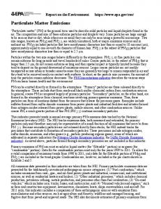
Figure (1): The 30-km northeast and southwest zone of Kerman cement factory Main Stages of Model Implementation • Control Pathway This section of the software specified the information such as the type of output (concentration, wet deposition, dry deposition, and total deposition), pollutant, mean time and statistical periods, and dispersion coefficients. In the present project, the type of concentration output and total suspended particulates (TSP) was determined and the 1-hour and 24-hour mean times as well as the one-year statistical period were selected. Furthermore, the parameter of dispersion coefficient was specified as a ‘rural’ option due to the fact that more that %50 of the land uses around the study site lacked urbanism within a 3-km radius and that the factory was situated outside the town. Then, the option of ‘elevated’ was selected due to the roughness in the intended site. In the following section, the premises of the model were confirmed and the required stages were accomplished

1

0/2625 0/0725 0/2625

In finale, with the implementation of this preprocessor, two files were created with SFC 4 and PFL 5 extensions that included all the meteorological parameters required for the model.

• Source Pathway The source pathway assessed and corrected the information of all emission sources as well as the effect of buildings and related parameters. Since the technical specifications of flues and their emission coefficients were introduced in the previous section of the software as a point source, this section of the software remained and was accepted unchanged.

Preliminary Stages Once the previous stage was accomplished the next stage of the present project was pursued in the main AERMOD VIEW software. In this section, a new operating file should be first introduced and defined in the software. Afterwards, it is necessary to determine the coordinate system and zone of the intended study site. The present study located the coordinate system on WGS84 and UTM the zone on 40 degrees north. In order to display the image of the intended study site as well as the overall location of the factory and its flues on the screen, a satellite image was taken on 07/06/2016 at 11:48 am from USGS website. Then several files specifying the factory zone and its flues on this image were imported to the GIS software. After editing, the image was saved in Google Earth to enter the AERMOD page (Figure 1). The project information was introduced using the input file to be processed by the model. First, the specifications of the flues in the center of the factory, including their geographical coordinates (latitude and longitude) were entered in meters. Next, based on the type of the selected pollutants in the source pathway, the information of the point sources (flues) including source name (flue), geographical latitude, longitude, flue height, flue diameter, velocity of exhaust gas, temperature of exhaust gas, and emission rate (Tables2 & 3) were entered as well. At this stage, once the velocity and diameter were entered, the software automatically calculated the rate of discharge. The emission rate per g/s can be obtained through multiplication of the rate of discharge by the concentration of suspended particles divided by 1000.

• Receptor Pathway The receptor pathway specified the important concentrations as well as the type and specifications of the receptor. Receptors are places where the model and concentrations of the pollutants are calculated. Homogenous receptor network was selected. A point in the center of the cement factory was selected as the coordinate point of origin. Then the receptors were specified in an area of 30×30 km2 (regional scale) with a network distance of 1000 m (3,721 network points) for either of direction X or Y. • Meteorology Pathway This section added the meteorological data of the intended site to the MET section in the form of two output files under SFC and PFL extensions that had been created in AERMET software.

• Output Pathway The output pathway specified the demonstration and characteristics of the output files (maximum concentration, alignment lines etc.) that were displayed in the model after implementation. In this pathway, the premises of the software were accepted. Table (2): List of monitoring points of exhaust suspended particles and location of sources in UTM coordinates (General Directorate of Environmental Protection, Tehran, 2014) No. Monitoring Points Geographical Geographical Longitude Latitude (m) (m) 1

4 5

2

Surface Data Upper Data

3

Electro-filter exhaust particles of furnace No. 1, preheater unit No. 1 Electro-filter exhaust particles of furnace No. 2, preheater unit No.

3344932

491280

3344713

491206

Khanaki. Sahar et al

3 4 5 6

2 Electro-filter exhaust particles of furnace No. 3, preheater unit No. 3 Exhaust particles of cement mill, cement mill unit, line No. 2 Exhaust particles of cement mill, cement mill unit, line No. 3 Exhaust particles of cement mill, cement mill unit, line No. 4

World J Environ Biosci, 2017, 6, (SI):1-9

3344863

491178

3344717

491162

3344797

491192

3344747

491189

with field measurement values. The evaluation was done using the statistical parameters proposed by US Environmental Protection Agency. Table (4): Location of the stations of measured data in UTM coordinates (General Directorate of Environmental Protection, Tehran, 2014) Station Longitude Latitude Station Name No. (m) (m) South side – 1 next to entrance 334507 491199 door West side – 2 across from the 3345042 490357 mine North side – 3 across from 3345518 491092 waste deposit East side – 4 across from 3345033 491662 clinker deposit

Table (3): Physical parameters of the flues of Kerman cement factory in AERMOD model (General Directorate of Environmental Protection, Tehran, 2014) Elect Ceme Ceme Paramet Ceme roElectro Electro nt nt ers of nt filter -filter 2 -filter 3 Mill Mill Flues Mill 4 1 2 3 Height of 44 72 90 25 34 31.5 Flue (m) Diameter of Flue 1.6 2.4 2.6 1.1 2 2 (m) Velocity of Exhaust 16.5 17.2 17.5 19.5 14.9 13.1 Gas (m/s) Temperat ure of 170.2 Exhaust 138.3 148.5 68 74 91 Gas (Kelvin) Emission

Rate (g/s)

2.45

13.2

8.73

1.65

3.8

Parameters in Comparison of Measured data with Predicted Data • Relative Fractional Bias The relative fractional bias was used to make the bias of the model dimensionless to reduce the bias of the model through Equation (1). Equation (1): As specified by EAP, the variations of relative fractional bias

ranged from -0.5 to +0.5 (Jampana et al., 2004).

• Normalized Mean Square Error (NMSE) The normalized mean square error represents the dispersion of all data that is indicated through Equations 2-3 (Jampana et al., 2004). Equation (2): As specified by EAP, the range of variations for NMSE was less

0.3

Implementation of AERMAP Preprocessor AERMAP is the second preprocessor is AERMOD model that analyzes the topographical data of the site. AERMAP preprocessor determines the height of all receptors and sources as well as the altitude scale of any receptor that has the greatest effect on the dispersion of pollutants in that receptor. In the terrain section, one DEM of the intended site with a precision of 90 meters in the form of SRTM3 type and HGT format was prepared using USGS website and was introduced to this preprocessor and implemented after separating the intended area. Topographical data were entered. The elevated alignment lines were plotted after entering the DEM (the heights were plotted precisely on the networks). Finally, once the accomplishment of all stages was ensured and the errors were resolved, the model was implemented in a general manner. The final simulated outputs were displayed on the image in the form of concentration alignment lines for all the specified mean times.

than 0.5 (Jampana et al., 2004).

• Factor of Two The factor of two is the percentage of the estimated value on the actual value that is shown through Equation (3). Equation (3): As specified by EAP, the range of variations for factor of two

was greater than 0.8 (Jampana et al., 2004). The best mode for the model is when the relative fractional bias and NMSE are equal to zero and when the bias of geometric mean and variance of geometric mean are equal to one (Jampana et al., 2004).

Comparison of Measured data with Predicted Data According to Table (4), four receptors were specified, in this study, to evaluate the results of simulation by AERMOD model

RESULTS

4

Khanaki. Sahar et al

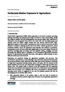
World J Environ Biosci, 2017, 6, (SI):1-9 the topographic map in Figure (3), the height of the intended site ranges from 1659 to 3576 meters. The highest areas are located in the northeast, southeast and northwest.

AERMOD model was implemented in the present study and its results were compared with Iran clean air standards and EPA standards. Finally, to ensure the results of the model, a comparison was made between the measured and predicted environmental data using the proposed EAP parameters.

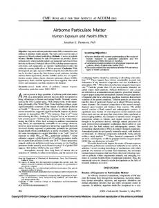
Windrose Interpretation Windrose is a diagram that illustrates the speed, direction and frequency of winds of a given location using a central coordinate system. According to Figure (2) that was plotted in 10 classes per m/s using WRPLOT View, the Windrose diagram displays that the prevailing wind direction was the north. The wind speeds under 3 m/s speed were considered as quiet winds with %33.3 frequency, wind speeds of 3-5 m/s had %41.3 frequency, wind speeds of 5-8 m/s had %21.6 frequency, wind speeds of 8-11.10 m/s/ had %3.4 frequency and wind speeds of over 11.10 m/s had %0.3 frequency.

Figure (3): Topographic map of the intended site Results of Predicted Concentrations Particles for Different Mean Times

of

Suspended

Figures 6 to 8 display the predicted concentrations of suspended particles for different mean times.

Predicted Concentrations of Suspended Particles for a 1-hour Mean Time The concentrations predicted by the model for a 1-hour mean time shows that the concentration dispersion ranges from 1 to 134 μg/m3 so that the maximum concentration i.e. (134) μg/m3, occurred with the longitude of 488315.1, latitude of 3345421 and height of 1811.5 m on 31/01/2014 at 3 o’clock. •

Figure (4): Predicted concentrations of suspended particle for a 1-hour mean time

Figure (2): Windrose diagram and frequency of wind speed classes

Predicted Concentrations of Suspended Particles for a 24-hours Mean Time The concentrations predicted by the model for a 24-hour mean time shows that the concentration dispersion ranges from 0.1 to 11.7 μg/m3 so that the maximum concentration i.e. (11.7) μg/m3, occurred with the longitude of 3346421, latitude of 487315 and height of 1898 m on 20/01/2014 at 24. •

Topographic Map The existing roughness on the ground surface and the presence of obstacles such as mountains etc. affect the emission of pollutants and they can be either harmful or beneficial depending on local and topographical conditions. According to

5

Khanaki. Sahar et al

World J Environ Biosci, 2017, 6, (SI):1-9 at 1

Table (6): Five of the first maximum concentrations for 24hour mean time Ran k

Longitud e (m)

Latitude (m)

Height (m)

Concentr ation (μg/m3)

1

487315

3346421

1898

11.7

3

491315.1

3344421

1754

8.85

5

491315.1

2

487315

4

Figure (5): Predicted concentrations of suspended particle for a 24-hour mean time

492315.1

1 2 3 4

489315.1

1

488315.1

3345421

1811.5

3

487315.1

3347421

1897.6

2 4 5

487315.1 489315.1 489315.1

3346421 3348421 3347421

134.4

1882.3

133.13

1887.2

71.77

1813.3

81.43 60.53

489315.1

Spring

Table (5): Five of the first maximum concentrations for 1hour mean time Concentration (μg/m3)

3345421

8.24

1743

7.60

3346421 3347421 3346421 3346421 3348421

1882.3 1897.6 1840.6

2.92 2.08 1.98

1841.4

1.42

1887.2

1.40

Table (8): Measured and predicted concentrations of PM10 environmental suspended particles Time of Place of Predicted Measured Measureme Measureme Concentratio Concentratio (μg/m3) (μg/m3)

Maximum Concentrations in Different temporal and Spatial Conditions Tables (5) to (7) present the first maximum simulated concentrations for 1-hour, 24-hour and one-year statistical periods. The predicted concentrations in different mean times show that height is an effective factor in the amount of higher concentrations. •

Height (m)

1754

9.09

Results of Comparison of Measured data with Predicted Data According to range specified by EAP for the relative fractional bias that varied from -0.5 to +0.5, the measured value of relative fractional bias was equal to +0.23; therefore, the simulation results were consistent with measurement results. The measured value of NMSE was less than the criterion specified by EAP (less than 0.5) which was equal to 0.0002 indicating the consistency of simulation results with the measurement results. The range of factor of two specified by EAP was greater than 0.8 i.e. the measured value of factor of two was equal to 0.8; therefore, the simulation results were consistent with measurement results.

Figure (6): Predicted concentrations of suspended particle for an annual mean time

Latitude (m)

3345421

487315.1 487315.1 488315.1

5

Longitude (m)

1992.3

20/01/201 4 at 24 15/10/201 4 at 24 05/02/201 4 at 24 05/11/201 4 at 24 12/03/201 4 at 24

Table (7): Five of the first maximum concentrations for annual mean time Rank Longitude Latitude Height Concentration (m) (m) (m) (μg/m3)

Predicted Concentrations of Suspended Particles for an Annual Mean Time The concentrations predicted by the model for an annual mean time shows that the concentration dispersion ranges from 0.03 to 2.92 μg/m3 so that the maximum concentration i.e. (2.92) μg/m3, occurred with the longitude of 487315.1, latitude of 3346421 and height of 1882.3 meters. •

Rank

3346421

Date

Summer

Date 31/01/2014 at 3 15/10/2014 at 4 10/01/2014 at 6 01/10/2014 at 21 11/02/2014

Fall Winter

6

Southside Westside Northside Eastside Southside Westside Northside Eastside Southside Westside Northside Eastside Southside Westside Northside

26.75 16.6 16.7 34 39.03 19.54 30.26 35 20.2 23 22.36 22.02 18.89 28.5 26.18

37 34 27 40 39 32 25 41 32 29 26 25 34 32 30

Khanaki. Sahar et al

World J Environ Biosci, 2017, 6, (SI):1-9

Eastside

27.43

Therefore, the maximum concentrations were only compared with these two mean time and period. Based on the simulated concentration of 11.7 μg/m3 for the 24-hour mean time in Table (6) and its comparison with EAP and Iran clean air standards, this pollutant was 4.37 times lower than Iran clean air standards and 12.82 times lower than EAP standards. Consequently, it did not cause any pollution. Furthermore, it was estimated as 2.92 μg/m3 for the annual statistical period, as shown in Table (7), indicating that it was 6 times lower than Iran clean air standards and did not cause any pollution.

29

Table (9): Comparison of measured data with predicted data Parameter Value FB

0.2303

NMSE

0.0002

Fa2

0.8

DISCUSSION

The present study intended to simulate the particulate matter dispersion emitted from fixed sources (flues) of Kerman cement factory using AERMOD model developed by the US environmental protection agency (EAP) that has been proposed as one of the advanced models. The AERMOD model was implemented using meteorological data of Kerman station in an area of 30×30 km2 (regional scale) with a distance of 1000 m (3721 network points) for 1-hour and 24-hour mean times as well as a one-year statistical period. Afterwards, the maximum concentrations simulated by the model were compared with EAP and Iran clean air standards. The simulation of pollutants concentrations for different mean times showed that the maximum concentrations occurred in the vicinity of the emission source. Moreover, the higher concentrations showed a tendency towards the south of emission source. The prevailing wind direction in the intended site was the north that was considered as an effective factor in transporting the pollutant of suspended particles to the south. Atabi et al. (2013) found that wind direction has a significant effect on the dispersion of pollutants. The comparison of the concentrations simulated by the mode with EAP and Iran clean air standards showed that the concentrations simulated by AERMOD model were significantly lower than the standard limit. The assessment of five maximum concentrations indicated that the elevated receptors (receptor with higher altitude) were affected by higher concentrations in the 24-hour mean time. Hekel et al. (2011) simulated the concentration of mercury element in residential areas using AERMOD model; they showed the significant effect of topography on the spatial dispersion of air pollution. Khebri et al. (2013), who studied the effect of digital elevation model on simulating air pollution using AERMOD model, found the same results. Ashrafi et al. (2012) investigated the sensitivity analysis of AERMOD model in estimating the dispersion of air pollution emitted from industries. They found that the higher the altitude of the receptors specified by the AERMAP preprocessor than the height under the flues, that area will be considered as a high area. Due to the same high altitude, the wind cannot disperse the pollutant mass properly. Therefore, the receptors receive higher concentrations. On the contrary, the lower the altitude of the receptors than the height under the flues, the area is a flat area where the wind flows well, disperses the pollutants properly and there will lead to lower concentrations. Environmental measurements showed that the maximum concentration of PM10 particulate matter respectively occurred in the eastside across from clinker deposit in the summer, eastside in the spring and Southside next to the entrance door in the summer which were lower than the 24-hour standard limit specified by EAP (150 μg/m3) and the annual standard limit specified by Iran clean air standards. The maximum predicted concentrations occurred in the Southside and eastside in the summer while in the eastside in the spring that were significantly lower than the EAP and Iran clean air standards. In an investigation into the TSP pollutants emitted

Table (10): Iran clean air standards for 2009, 2010 and 2011 2009 2010 2011 Mean Pollu Time μg/ PP μg/ μg/ tant PPM PPM (Max.) m3 M m3 m3 8-hour 1000 9 1000 9 1000 9 CO 1-hour 4000 35 4000 35 4000 35 NO2 SO2

PM10

PM2.5

Annual

100

0.05

60

0.031

40

0.021

24-hour

365

0.14

250

0.094

100

0.037

-

12

-

10

1-hour

Annual Annual

24-hour Annual

24-hour

-

80 50

150 -

150

-

0.30 -

-

50 40 90 30

-

0.019 -

-

20

20 50

-

0.007

25

-

Table (11): Environmental air quality standards specified by EAP Pollutant Mean Time Standard EAP (Max.) PPM μg/m3 CO 8-hour 9 1-hour 35 NO2 Annual 0.53 1-hour 0.1 SO2 Annual 24-hour 0.075 PM10 Annual 24-hour 150 PM2.5 Annual 12 24-hour 35

Comparison of Maximum Concentrations with Iran Clean Air Standards and EAP Standards In this section, once the outputs were specified and the concentration balance curves were demonstrated for different mean times, the maximum concentrations specified by both EAP and Iran clean air standards were compared with each other, as shown in Tables (10) and (11). It should be noted that according to EAP and Iran clean air standards, there are two permitted standard limits for the pollutant of particulate matter. The concentrations simulated by the model in the present study were compared with PM10 (because the particulate matter was measured less than 10 microns). On the other hand, the statistical mean times and periods (1-hour, 24hour and annual) were simulated using AERMOD model in the present study; however, according to both tables of EAP and Iran clean air standards, there is only a threshold limit of 24hour mean time and one-year period for particulate matter.

7

Khanaki. Sahar et al

World J Environ Biosci, 2017, 6, (SI):1-9

from flue exhausts of a cement factory based on AERMOD model, the results of Nourpour’s et al. (2014) simulation showed that the concentration of pollutants were significantly lower than the limit of Iran clean air standards.

10.

CONCLUSION

11.

Dispersion of air pollutants in industrial units is one of the factors that constantly affects the environment and the ecosystems of the adjacent areas and can endanger the lives of people living in the vicinity of such units in the long run. Pollution dispersion models are useful tools for understanding the pollutants behaviors after being emitted from the sources and make the excessive and expensive measurements unnecessary. In the present study, the AERMOD dispersion model is an appropriate model for determining the average annual and hourly concentrations of PM10 particles emitted from the point sources. In general, according to the predictions, it can be stated that AERMOD software was efficient in predicting the concentration of pollutants. Therefore, AERMOD dispersion model can be used as an appropriate scientific tool for the analysis of control and policy-making strategies in order to reduce and prevent air pollution.

12. 13. 14.

REFERENCES

1. 2.

3.

4. 5. 6. 7. 8. 9.

15.

Abril GA, Wannaz ED, Mateos AC, Pignata ML. Biomonitoring of airborne particulate matter emitted from a cement plant and comparison with dispersion modelling results. Atmos Environ 2014; 82: 154-63. Ashrafi, Kh., Shafipour, M., Salimian, M. & Momeni, M. (2012). Determining the emission rate and simulating dispersion of pollutants of organic compound emitted from surface evaporation of reservoirs located in Assaluyeh. Ecology, 38(3), 4760. Atabi, F., Jafari Gol, F., Momeni, M. R., Salimian, M. & Bahman Niagh, R. (2013). Simulation of CO pollutant dispersion using AERMOD in south Pars gas refinery No, 4 in Assaluyeh. Journal of environmental health engineering, 1(4). School of environment and energy. Islamic Azad University, science and Research Branch, Tehran, Iran. Baroutian S, Mohebi A, Goharrizi SA.Measuring and modeling particulate dispersion a case study of Kerman cement plant. J Hazard Mater 2006;136:468-74. Daryanoosh SM, Goudarzi G, Omidikhaniabadi Y, Armin H, Bassiri H, Khaniabadi FO. Effect of exposure to PM10 on cardiovascular diseases hospitalizations in Ahvaz Khorramabad andIlam Iran During 2014. IJHSE 2016;3:428-33. dioxide:Summary of risk assessment, Global update.World Health Organization.http://www.euro.who.int/ documen Available at /E87950. pdf. Engelbrecht J, Joubert J, Harmse J,Hongoro C. Optimising a fall out dust monitoring sampling programme at acement manufacturing plant in South Africa. Afr J Environ Sci Technol 2013;7: 12839. General Directorate of Environmental Protection. (2014). Environmental Pollution Surveillance Office. Tehran. Ghermandi G, Fabbi S, Zaccanti M, Bigi A, Teggi S. Micro–scale simulation of atmospheric emissions

16. 17. 18.

19.

20. 21.

22.

23.

24.

25.

8

from power plant stacks in the Po Valley. APR 2015;6:6-11. Heckel PF, LeMasters GK. 2011. The use of AERMOD air pollution dispersion models to estimate residential ambient concentrations of elemental mercury. Water, Air, & Soil Pollution, 219:377_388. Isikli B, Demir T, Akar T, Berber A, Urer S, Kalyoncu C, et al. Cadmium exposure from the cement dust emissions a field study in a rural residence. Chemosphere2006;63:1546-52. Mwaiselage J, Bratveit M, Moen B, Mashalla Y. Cement dust exposure and ventilator function impairment an exposure response study. J Occup Environ Med2004; 46:658-67. Jampana, S.S., Kumar, A. and Varadarjan, C. 2004. Application of the united states environmental protection agencys AERMOD model to an industrial Area, Environmental Progress, vol .23,pp. 141-152. Khebri, Z., Mousavian Nodoushan, N., Nejad Kouraki, F. & Mansouri, N. (2013). The effect of digital elevation model on air pollution modelling using AERMOD model. Remote sensing and geographic information system in natural resources, 4(4). Mohebbi A, Baroutian S. A detailed investigation of particulate dispersion from Kerman cement plant. Iran J Chem Chem Eng 2006;3:65-74. Momeni, E., Daneh Kar, E., Karimi, S. & Khorasani, N. E. (2013). Simulation of SO2 dispersion emitted from Ramin power plant of Ahwaz using AERMOD model. Journal of human and environment, 18, 3-8. Nourmoradi H, Goudarzi G, Daryanoosh SM, Omidikhaniabadi F, Jourvand M, Omidikhaniabadi Y. Health impacts of particulate matter in air by AirQ model in Khorramabad city Iran. J Bas Res Med Sci 2015; 2:44-52. Perez P, Reyes J.An integrated neural network model for PM10 forecasting. Atmos Environ 2006;40:284551. Statistical Center of Iran. (2011). Results of general census. Taiwo AM, Harrison RM, Shi Z. A review of receptor modelling of industrially emitted particulate matter. Atmos Environ 2014;97:109-20. U.S. Environmental Protection Agency. 2015. Technology Transfer Network, Support Center for Regulatory Atmospheric Modeling. Availabel from: http://www3.epa.gov/scram001/aqmindex.htm [Accessed 14 October 2015]. U.S. Environmental Protection Agency. 2004. User guide for the AERMOD METEOROLOGICAL PREPROCESSOR (AERMET). Research Triangle Park, North Carolina: Office of Air Quality Planning and Standards, Emissions Monitoring and Analysis Division EPA-454/B-03-002, 252 pp. U.S. Environmental Protection Agency.2015.Air Quality Management Online Portal. Available US Environmental Protection Agency. 2004. USER’S GUIDE FOR THE AMS/EPA REGULATORY MODELAERMOD, Office of Air Quality Planning and Standards, Emissions Monitoring and Analysis Division, Research Triangle Park North Carolina, EPA-454/B-03-001, 216 pp. WHO Air quality guidelines for particulate matter. 2005. ozone, nitrogen dioxide and sulfur World Health Organization. 2014. 7 million premature deaths annually linked toairpollution. Available from:

Khanaki. Sahar et al

World J Environ Biosci, 2017, 6, (SI):1-9

http://www.who.int/mediacentre/news/releases/2 014/air-pollution/en/. [Accessed 25 March 2014]. 26. www. Noaa.gov 27. Yazdanparast T, Salehpour S, Masjedi MR, Azin SA, Seyedmehdi SM, Boyes E, et al. Air pollution: the knowledge and ideas of students in Tehran-Iran, and a comparison with other countries. Acta Med Iran 2013;51:487-93.

9