Dec 10, 2017 - form to avoid expensive Gaussian elimination during simulation. The main ... computed in parallel and lend themselves to distributed.
1
Simulation of Quantum Circuits via Stabilizer Frames ´ Hector J. Garc´ıa Igor L. Markov University of Michigan, EECS, Ann Arbor, MI 48109-2121 {hjgarcia, imarkov}@eecs.umich.edu
arXiv:1712.03554v1 [cs.DS] 10 Dec 2017
F
Abstract—Generic quantum-circuit simulation appears intractable for conventional computers and may be unnecessary because useful quantum circuits exhibit significant structure that can be exploited during simulation. For example, Gottesman and Knill identified an important subclass, called stabilizer circuits, which can be simulated efficiently using group-theory techniques and insights from quantum physics. Realistic circuits enriched with quantum error-correcting codes and fault-tolerant procedures are dominated by stabilizer subcircuits and contain a relatively small number of non-Clifford components. Therefore, we develop new data structures and algorithms that facilitate parallel simulation of such circuits. Stabilizer frames offer more compact storage than previous approaches but require more sophisticated bookkeeping. Our implementation, called Quipu, simulates certain quantum arithmetic circuits (e.g., reversible ripple-carry adders) in polynomial time and space for equal superpositions of n-qubits. On such instances, known linear-algebraic simulation techniques, such as the (state-ofthe-art) BDD-based simulator QuIDDPro, take exponential time. We simulate quantum Fourier transform and quantum fault-tolerant circuits using Quipu, and the results demonstrate that our stabilizer-based technique empirically outperforms QuIDDPro in all cases. While previous high-performance, structure-aware simulations of quantum circuits were difficult to parallelize, we demonstrate that Quipu can be parallelized with a nontrivial computational speedup.
1
I NTRODUCTION
Quantum information processing manipulates quantum states rather than conventional 0-1 bits. It has been demonstrated with a variety of physical technologies (NMR, ion traps, Josephson junctions in superconductors, optics) and used in recently developed commercial products. Examples of such products include MagiQ’s quantum key distribution system and ID-Quantique’s quantum random number generator. Shor’s factoring algorithm [24] and Grover’s search algorithm [13] apply the principles of quantum information to carry out computation asymptotically more efficiently than conventional computers. These developments fueled research efforts to design, build and program scalable quantum computers. Due to the high volatility of quantum information, quantum error-correcting codes (QECC) and effective fault-tolerant (FT) architectures are necessary to build reliable quantum computers. For instance, the work in [22] describes practical FT architectures for quantum computers, and [15] explores architectures for constructing reliable communication channels via distribution of high-fidelity EPR pairs in a large quantum
computer. Most quantum algorithms are described in terms of quantum circuits and, just like conventional digital circuits, require functional simulation to determine the best FT design choices given limited resources. In particular, high-performance simulation is a key component in quantum design flows [25] that facilitates analysis of trade-offs between performance and accuracy. Simulating quantum circuits on a conventional computer is a difficult problem. The matrices representing quantum gates, and the vectors that model quantum states grow exponentially with an increase in the number of qubits – the quantum analogue of the classical bit. Several software packages have been developed for quantumcircuit simulation including Oemer’s Quantum Computation Language (QCL) [21] and Viamontes’ Quantum Information Decision Diagrams (QuIDD) implemented in the QuIDDPro package [26]. While QCL simulates circuits directly using state vectors, QuIDDPro uses a variant of binary decision diagrams to store state vectors more compactly in some cases. Since the state-vector representation requires excessive computational resources in general, simulation-based reliability studies (e.g. faultinjection analysis) of quantum FT architectures using general-purpose simulators has been limited to small quantum circuits [5]. Therefore, designing fast simulation techniques that target quantum FT circuits facilitates more robust reliability analysis of larger quantum circuits. Stabilizer circuits and states. Gottesman [12] and Knill identified an important subclass of quantum circuits, called stabilizer circuits, which can be simulated efficiently on classical computers. Stabilizer circuits are exclusively composed of Clifford gates – Hadamard, Phase and controlled-NOT gates (Figure 1) followed by onequbit measurements in the computational basis. Such cir-
1 H= √ 2
�
1 1
�
1 −1
� 1 P = 0
0 i
�
1 0 CN OT = 0 0
0 1 0 0
0 0 0 1
0 0 1 0
Fig. 1. Clifford gates: Hadamard (H), Phase (P) and controlled-NOT (CNOT).
2
cuits are applied to a computational basis state (usually |00...0i) and produce output states known as stabilizer states. Because of their extensive applications in QECC and FT architectures, stabilizer circuits have been studied heavily [1], [12]. Stabilizer circuits can be simulated in polynomial-time by keeping track of the Pauli operators that stabilize1 the quantum state. Such stabilizer operators are maintained during simulation and uniquely represent stabilizer states up to an unobservable global phase.2 Thus, this technique offers an exponential improvement over the computational resources needed to simulate stabilizer circuits using vector-based representations. Aaronson and Gottesman [1] proposed an improved technique that uses a bit-vector representation to simulate stabilizer circuits. Aaronson implemented this simulation approach in his CHP software package. Compared to other vector-based simulators (QuIDDPro, QCL) the technique in [1] does not maintain the global phase of a state and simulates each Clifford gate in Θ(n) time using Θ(n2 ) space. The overall runtime of CHP is dominated by measurements, which require O(n2 ) time to simulate.
for input states consisting of equal superpositions of computational-basis states. On such instances, wellknown generic simulation techniques take exponential time. We simulate various quantum Fourier transform and quantum fault-tolerant circuits, and the results demonstrate that our data structure leads to ordersof-magnitude improvement in runtime and memory as compared to state-of-the-art simulators. In the remaining part of this document, we assume at least a superficial familiarity with quantum computing. Section 2 describes key concepts related to quantumcircuit simulation and the stabilizer formalism. In Section 3, we introduce stabilizer frames and describe relevant algorithms. Section 4 describes in detail our simulation flow implemented in Quipu, and Section 5 discusses a parallel implementation of our technique. In Section 6, we describe empirical validation of Quipu and in single- and multi-threaded variants, as well as comparisons with state-of-the-art simulators. Section 7 closes with concluding remarks.
Stabilizer-based simulation of generic circuits. We propose a generalization of the stabilizer formalism that admits simulation of non-Clifford gates such as Toffoli3 gates. This line of research was first outlined in [1], where the authors describe a stabilizer-based representation that stores an arbitrary quantum state as a sum of density-matrix4 terms. In contrast, we store arbitrary states as superpositions5 of pure stabilizer states. Such superpositions are stored more compactly than the approach from [1], although we do not handle mixed stabilizer states. The key obstacle to the more efficient pure-state approach has been the need to maintain the global phase of each stabilizer state in a superposition, where such phases become relative. We develop a new algorithm to overcome this obstacle. We store stabilizer-state superpositions compactly using our proposed stabilizer frame data structure. To speed up relevant algorithms, we store generator sets for each stabilizer frame in row-echelon form to avoid expensive Gaussian elimination during simulation. The main advantages of using stabilizer-state superpositions to simulate quantum circuits are: (1) Stabilizer subcircuits are simulated with high efficiency. (2) Superpositions can be restructured and compressed on the fly during simulation to reduce resource requirements. (3) Operations performed on such superpositions can be computed in parallel and lend themselves to distributed or asynchronous processing. Our stabilizer-based technique simulates certain quantum arithmetic circuits in polynomial time and space
2
1. An operator U is said to stabilize a state iff U |ψi = |ψi. 2. According to quantum physics, the global phase exp(iθ) of a quantum state is unobservable and does not need to be simulated. 3. The Toffoli gate is a 3-bit gate that maps (a, b, c) to (a, b, c ⊕ (ab)). 4. Density matrices are self-adjoint positive-semidefinite matrices of trace 1.0, that describe the statistical state of a quantum system [19]. 5. A superposition is a norm-1 linear combination of terms.
BACKGROUND
AND
P REVIOUS W ORK
Quantum information processes, including quantum algorithms, are often modeled using quantum circuits and, just like conventional digital circuits, are represented by diagrams [19], [26]. Quantum circuits are sequences of gate operations that act on some register of qubits – the basic unit of information in a quantum system. The quantum state |ψi of a single qubit is described by a twodimensional complex-valued vector. In contrast to classical bits, qubits can be in a superposition of the 0 and 1 states. Formally, |ψi = α0 |0i + α1 |1i, where |0i = (1, 0)> and |1i = (0, 1)> are the two-dimensional computational basis states and αi are probability amplitudes that satisfy |α0 |2 +|α1 |2 = 1. An n-qubit register is the tensor product of n single qubits and thus is modeled by a complex P2n −1 vector |ψ n i = |ψ1 i ⊗ · · · ⊗ |ψn i = i=0 αi |bi i, where each bi is a binary string representing the value i of each P2n −1 basis state. Furthermore, |ψ n i satisfies i=0 |αi |2 = 1. Each gate operation or quantum gate is a unitary matrix that operates on a small subset of the qubits in a register. For example, the quantum analogue of a NOT gate is the operator X = ( 01 10 ), X⊗I
α0 |00i + α1 |10i 7−−−→ α0 |10i + α1 |00i Similarly, the two-qubit CNOT operator flips the second qubit (target) iff the first qubit (control) is set to 1, e.g., CN OT
α0 |00i + α1 |10i 7−−−−→ α0 |00i + α1 |11i Another operator of particular importance is the Hadamard (H), which is frequently used to put a qubit in a superposition of computational-basis states, e.g., I⊗H
α0 |00i + α1 |10i 7−−−→
α0 (|00i + |01i) + α1 (|10i + |11i) √ 2
3
Note that the H gate generates unbiased superpositions in the sense that the squares of the absolute value of the amplitudes are equal. The dynamics involved in observing a quantum state are described by non-unitary measurement operators [19, Section 2.2.3]. There are different types of quantum measurements, but the type most pertinent to our discussion comprises projective measurements in the computational basis, i.e., measurements with respect to the |0i or |1i basis states. The corresponding measurement operators are P0 = ( 10 00 ) and P1 = ( 00 01 ), respectively. The probability p(x) of obtaining outcome x ∈ {0, 1} on the j th qubit of state |ψi is given by the inner product hψ| Pxj |ψi, where hψ| is the conjugate transpose of |ψi. For example, the probability of obtaining |1i upon measuring |ψi = α0 |0i + α1 |1i is
and amplitudes. The symmetries are operators for which these states are 1-eigenvectors. Algebraically, symmetries form group structures, which can be specified compactly by group generators [14].
p(1) = (α0∗ , α1∗ )P1 (α0 , α1 )> = (0, α1∗ )(α0 , α1 )> = |α1 |2
Observe that I stabilizes all states and −I does not stabi√ lize any state. Thus, the entangled state (|00i + |11i)/ 2 is stabilized by the Pauli operators X ⊗X, −Y ⊗Y , Z ⊗Z and I ⊗I. As shown in Table 1, it turns out that the Pauli matrices along with I and the multiplicative factors ±1, ±i, form a closed group under matrix multiplication [19]. Formally, the Pauli group Gn on n qubits consists of the nfold tensor product of Pauli matrices, P = ik P1 ⊗ · · · ⊗ Pn such that Pj ∈ {I, X, Y, Z} and k ∈ {0, 1, 2, 3}. For brevity, the tensor-product symbol is often omitted so that P is denoted by a string of I, X, Y and Z characters or Pauli literals, and a separate integer value k for the phase ik . This string-integer pair representation allows us to compute the product of Pauli operators without explicitly computing the tensor products,6 e.g., (−IIXI)(iIY II) = −iIY XI. Since | Gn |= 4n+1 , Gn can have at most log2 | Gn |= log2 4n+1 = 2(n + 1) irredundant generators [19]. The key idea behind the stabilizer formalism is to represent an n-qubit quantum state |ψi by its stabilizer group S(|ψi) – the subgroup of Gn that stabilizes |ψi. Theorem 1: For an n-qubit pure state |ψi and k ≤ n, S(|ψi) ∼ = Zk2 . If k = n, |ψi is specified uniquely by S(|ψi) and is called a stabilizer state. Proof: (i) To prove that S(|ψi) is commutative, let P, Q ∈ S(|ψi) such that P Q |ψi = |ψi. If P and Q anticommute, -QP |ψi = -Q(P |ψi) = -Q |ψi = -|ψi = 6 |ψi. Thus, P and Q cannot both be elements of S(|ψi). (ii) To prove that every element of S(|ψi) is of degree 2, let P ∈ S(|ψi) such that P |ψi = |ψi. Observe that
Cofactors of quantum states. The output states obtained after performing computational-basis measurements are called cofactors, and are states of the form |0i |ψ0 i and |1i |ψ1 i. These states are orthogonal to each other and add up to the original state. The norms of cofactors and the original state are subject to the Pythagorean c=0 � theorem. c=1We � denote the |0i- and |1i-cofactor by ψ and ψ , respectively, where c is the index of the measured qubit. One can also consider cofactors, qr=00 � qr=01iterated � qr=10 � ψ ψ ψ such as double cofactors , , and qr=11 � ψ . Cofactoring with respect to all qubits produces amplitudes of individual basis vectors. Readers familiar with cofactors of Boolean functions can use intuition from logic optimization and Boolean function theory. 2.1
Quantum circuits and simulation
To simulate a quantum circuit C, we first initialize the quantum system to some desired state |ψi (usually a basis state). |ψi can be represented using a fixed-size data structure (e.g., an array of 2n complex numbers) or a variable-size data structure (e.g., algebraic decision diagram). We then track the evolution of |ψi via its internal representation as the gates in C are applied one at a time, eventually producing the output state C |ψi [1], [19], [26]. Most quantum-circuit simulators [8], [20], [21], [26] support some form of the linear-algebraic operations described earlier. The drawback of such simulators is that their runtime and memory requirements grows exponentially in the number of qubits. This holds true not only in the worst case but also in practical applications involving quantum arithmetic and quantum FT circuits. Gottesman developed a simulation method involving the Heisenberg model [12] often used by physicists to describe atomic-scale phenomena. In this model, one keeps track of the symmetries of an object rather than represent the object explicitly. In the context of quantum-circuit simulation, this model represents quantum states by their symmetries, rather than complex-valued vectors
2.2
The stabilizer formalism
A unitary operator U stabilizes a state |ψi iff |ψi is a 1–eigenvector of U , i.e., U |ψi = |ψi. We are interested in operators U derived from �the Pauli matrices: � 1 0 X = ( 01 10 ) , Y = 0i −i 0 −1 , and the identity 0 ,Z = 1 0 I = ( 0 1 ). The one-qubit states stabilized by the Pauli matrices are: √ √ X : (|0i + |1i)/ √2 −X : (|0i − |1i)/ √2 Y : (|0i + i |1i)/ 2 −Y : (|0i − i |1i)/ 2 Z : |0i −Z : |1i
6. This holds true due to the identity: (A⊗B)(C ⊗D) = (AC ⊗BD).
TABLE 1 Multiplication table for Pauli matrices. Shaded cells indicate anticommuting products. I X Y Z
I I X Y Z
X X I −iZ iY
Y Y iZ I −iX
Z Z −iY iX I
4
P 2 = il I for l ∈ {0, 1, 2, 3}. Since P 2 |ψi = P (P |ψi) = P |ψi = |ψi, we obtain il = 1 and P 2 = I. (iii) From group theory, a finite Abelian group with identity element e such that a2 = e for every element a in the group must be ∼ = Zk2 . (iv) We now prove that k ≤ n. First note that each independent generator P ∈ S(|ψi) imposes the linear constraint P |ψi = |ψi on the 2n -dimensional vector space. The subspace of vectors that satisfy such a constraint has dimension 2n−1 , or half the space. Let gen(|ψi) be the set of generators for S(|ψi). We add independent generators to gen(|ψi) one by one and impose their linear constraints, to limit |ψi to the shared 1-eigenvector. Thus the size of gen(|ψi) is at most n. In the case |gen(|ψi)| = n, the n independent generators reduce the subspace of possible states to dimension one. Thus, |ψi is uniquely specified. The proof of Theorem 1 shows that S(|ψi) is specified by only log2 2n = n irredundant stabilizer generators. Therefore, an arbitrary n-qubit stabilizer state can be represented by a stabilizer matrix M whose rows represent a set of generators Q1 , . . . , Qn for S(|ψi). (Hence we use the terms generator set and stabilizer matrix interchangeably.) Since each Qi is a string of n Pauli literals, the size of the matrix is n × n. The fact that Qi ∈ S(|ψi) implies that the leading phase of Qi can only be ±1 and not ±i.7 Therefore, we store the phases of each Qi separately using a binary vector of size n. The storage cost for M is Θ(n2 ), which is an exponential improvement over the O(2n ) cost often encountered in vector-based representations. √
Example 1. The state |ψi = (|00i + |11i)/ 2 is uniquely XX specified by any of the following matrices: M1 = + + [ ZZ ], + XX − YY M2 = − [ Y Y ], M3 = + [ ZZ ]. One obtains M2 from M1 by left-multiplying the second row by the first. Similarly, M3 is obtained from M1 or M2 via row multiplication. Observe that multiplying any row by itself yields II, which stabilizes |ψi. However, II cannot be used as a generator because it is redundant and carries no information about the structure of |ψi. This holds true in general for M of any size. Theorem 1 suggests that Pauli literals can be represented using two bits, e.g., 00 = I, 01 = Z, 10 = X and 11 = Y . Therefore, a stabilizer matrix can be encoded using an n × 2n binary matrix or tableau. This approach induces a linear map Z2n 2 7→ Gn because vector addition in Z22 is equivalent to multiplication of Pauli operators up to a global phase. The tableau implementation of the stabilizer formalism is covered in [1], [19]. Observation 1. Consider a stabilizer state |ψi represented by a set of generators of its stabilizer group S(|ψi). Recall from the proof of Theorem 1 that, since S(|ψi) ∼ = Zn2 , each generator imposes a linear constraint on |ψi. Therefore, the set of generators can be viewed as 7. Suppose the phase of Qi is ±i, then Q2i =-I ∈ S(|ψi) which is not possible since -I does not stabilize any state.
(a)
(b)
Fig. 2. (a) Stabilizer-matrix structure for basis states. (b) Row-echelon form for stabilizer matrices. The X-block contains a minimal set of generators with X/Y literals. Generators with Z/I literals only appear in the Z-block. a system of linear equations whose solution yields the 2k (for some k between 0 and n) non-zero computationalbasis amplitudes that make up |ψi. Thus, one needs to perform Gaussian elimination to obtain such basis amplitudes from a generator set. Canonical stabilizer matrices. Observe from Example 1 that, although stabilizer states are uniquely determined by their stabilizer group, the set of generators may be selected in different ways. Any stabilizer matrix can be rearranged by applying sequences of elementary row operations in order to obtain the row-reduced echelon form structure depicted in Figure 2b. This particular stabilizer-matrix structure defines a canonical representation for stabilizer states [10], [12]. The elementary row operations that can be performed on a stabilizer matrix are transposition, which swaps two rows of the matrix, and multiplication, which left-multiplies one row with another. Such operations do not modify the stabilizer state and resemble the steps performed during a Gaussian elimination8 procedure. Several row-echelon (standard) forms for stabilizer generators along with relevant algorithms to obtain them have been introduced in the literature [3], [12], [19]. Stabilizer-circuit simulation. The computational-basis states are stabilizer states that can be represented by the stabilizer-matrix structure depicted in Figure 2a. In this matrix form, the ± sign of each row along with its corresponding Zj -literal designates whether the state of the j th qubit is |0i (+) or |1i (−). Suppose we want to simulate circuit C. Stabilizer-based simulation first initializes M to specify some basis state. Then, to simulate the action of each gate U ∈ C, we conjugate each row Qi of M by U .9 We require that the conjugation U Qi U † maps to another string of Pauli literals so that the resulting matrix M0 is well-formed. It turns out that the H, P and CNOT gates have such mappings, i.e., these gates conjugate the Pauli group onto itself [12], [19]. Table 2 lists mappings for the H, P and CNOT gates. Example 2. Suppose we simulate a CNOT gate on |ψi = 8. Since Gaussian elimination essentially inverts the n × 2n matrix, this could be sped up to O(n2.376 ) time by using fast matrix inversion algorithms. However, O(n3 )- time Gaussian elimination seems more practical. 9. Since Qi |ψi = |ψi, the resulting state U |ψi is stabilized by U Qi U † because (U Qi U † )U |ψi = U Qi |ψi = U |ψi.
5
√ (|00i+|11i)/ 2. Using the stabilizer representation, Mψ = � � � +XX � CN OT 0 7−−−−→ M0ψ = +XI +IZ . The rows of Mψ stabilize +ZZ √ CN OT |ψi 7−−−−→ (|00i + |10i)/ 2 as required.
Since H, P and CNOT gates are directly simulated via the stabilizer formalism, these gates are also known as stabilizer gates and any circuit composed exclusively of such gates is called a unitary stabilizer circuit. Table 2 shows that at most two columns of M are updated when a Clifford (stabilizer) gate is simulated. Therefore, such gates are simulated in Θ(n) time. Furthermore, for any pair of Pauli operators P and Q, P QP † = (−1)c Q, where c = 0 if P and Q commute, and c = 1 otherwise. Thus, Pauli gates can also be simulated in linear time as they only permute the phase vector of the stabilizer matrix. Theorem 2: An n-qubit stabilizer state |ψi can be ob⊗n tained by applying a stabilizer circuit to the |0i computational-basis state. Proof: The work in [1] represents the generators using a tableau, and then shows how to construct a canonical stabilizer circuit C from the tableau. We refer the reader to [1, Theorem 8] for details of the proof. Algorithms for obtaining more compact canonical circuits are discussed in [11]. Corollary 3: An n-qubit stabilizer state |ψi can be transformed by Clifford gates into the |00 . . . 0i computational-basis state. Proof: Since every stabilizer state can be produced by ⊗n applying some unitary stabilizer circuit C to the |0i state, it suffices to reverse C to perform the inverse transformation. To reverse a stabilizer circuit, reverse the order of gates and replace every P gate with P P P . The stabilizer formalism also admits measurements in the computational basis [12]. Conveniently, the formalism avoids the direct computation of measurement operators and inner products (Section 2). However, the updates to M for such gates are not as efficient as for Clifford gates. Note that any qubit j in a stabilizer state is either in a |0i (|1i) state or in an unbiased superposition of both. The former case is called a deterministic outcome and the latter a random outcome. We can tell these cases apart in Θ(n) time by searching for X or Y literals in the j th column of M. If such literals are found, the qubit must be in a superposition and the outcome is random with equal probability (p(0) = p(1) = .5); otherwise the outcome is deterministic (p(0) = 1 or p(1) = 1).
TABLE 2 Conjugation of Pauli-group elements by Clifford gates [19]. For the CN OT case, subscript 1 indicates the control and 2 the target. G ATE H
P
I NPUT X Y Z X Y Z
O UTPUT Z -Y X Y -X Z
G ATE
CN OT
I NPUT I1 X2 X1 I2 I1 Y2 Y1 I2 I1 Z2 Z1 I2
O UTPUT I1 X2 X1 X2 Z1 Y2 Y1 X2 Z1 Z2 Z1 I2
Case 1 – randomized outcomes: one flips an unbiased coin to decide the outcome x ∈ {0, 1} and then updates M to make it consistent with the outcome. Let Rj be a row in M with an X/Y literal in its j th position, and let Zj be the Pauli operator with a Z literal in its j th position and I everywhere else. The phase of Zj is set to +1 if x = 0 and −1 if x = 1. Observe that Rj and Zj anticommute. If any other rows in M anticommute with Zj , multiply them by Rj to make them commute with Zj . Then, replace Rj with Zj . Since this process requires up to n row multiplications, the overall runtime is O(n2 ). Case 2 – deterministic outcomes: no updates to M are necessary but we need to figure out whether the qubit is in the |0i or |1i state, i.e., whether the qubit is stabilized by Z or -Z. One approach is to perform Gaussian elimination (GE) to put M in row-echelon form. This removes redundant literals from M and makes it possible to identify the row containing a Z in its j th position and I’s everywhere else. The ± phase of such a row decides the outcome of the measurement. Since this is a GE-based approach, it takes O(n3 ) time in practice. The work in [1] improved the runtime of deterministic measurements by doubling the size of M to include n destabilizer generators in addition to the n stabilizer generators. Such destabilizer generators help identify which specific row multiplications to compute in order to decide the measurement outcome. This approach avoids GE and thus deterministic measurements are computed in O(n2 ) time. In Section 3, we describe a different approach that computes such measurements in linear time without extra storage but with an increase in runtime when simulating Clifford gates. In quantum mechanics, the states eiθ |ψi and |ψi are considered phase-equivalent because eiθ does not affect the statistics of measurement. Since the stabilizer formalism simulates Clifford gates via their action-byconjugation, such global phases are not maintained. Example 3. Suppose we have state |1i, which is stabilized by -Z. Conjugating the stabilizer by the Phase gate yields P (-Z)P † =-Z. However, in the state-vector P representation, |1i 7− → i |1i. Thus the global phase i is not maintained by the stabilizer. Since global phases are unobservable, they do not need to be maintained when simulating a single stabilizer state. However, in Section 4, we show that such phases must be maintained when dealing with stabilizer-state superpositions, where global phases become relative.
3
S TABILIZER F RAMES : DATA S TRUCTURE AND A LGORITHMS The Clifford gates by themselves do not form a universal set for quantum computation [1], [19]. However, the Hadamard and Toffoli (T OF ) gates do [2]. To simulate T OF and other non-Clifford gates, we extend the formalism to include the representation of arbitrary quantum
6
states as superpositions of stabilizer states. Example 4. Recall from Section 2.2 that computationalbasis states are stabilizer states. Thus, any one-qubit state |ψi = α0 |0i + α1 |1i is a superposition of the stabilizer states |0i and |1i. In general, any state decomposition in a computational basis is a stabilizer superposition. Suppose |ψi in Example 4 is an unbiased state such that α0 = ik α1 where k = {0, 1, 2, 3}. Then |ψi can be represented using a single stabilizer state instead of two (up to a global phase). The key idea behind our technique is to identify and compress large unbiased superpositions on the fly during simulation to reduce resource requirements. To this end, we leverage the following observation and derive a compact data structure for representing stabilizer-state superpositions. Observation 2. Given an n-qubit stabilizer state |ψi, there exists an orthonormal basis including |ψi and consisting entirely of stabilizer states. One such basis is obtained directly from the stabilizer of |ψi by changing the signs of an arbitrary, non-empty subset of generators of S(|ψi), i.e., by modifying the phase vector of the stabilizer matrix for |ψi.10 Thus, one can produce 2n −1 additional orthogonal stabilizer states. Such states, together with |ψi, form an orthonormal basis. This basis is unambiguously specified by a single stabilizer state, and any one basis state specifies the same basis. Definition 1. An n-qubit stabilizer frame F is a set of k ≤ 2n stabilizer states {|ψj i}kj=1 that forms an orthogonal subspace basis in the Hilbert space. We represent F by a pair consisting of (i) a stabilizer matrix M and (ii) a set of distinct phase vectors {σj }kj=1 , where σj ∈ {±1}n . We use Mσj to denote the ordered assignment of the elements in σj as the (±1)-phases of the rows in M. Therefore, state |ψj i is represented by Mσj . The size of the frame, which we denote by |F|, is equal to k. Each phase vector σj can be viewed as a binary (0-1) encoding of the integer index that denotes the respective basis vector. Thus, when dealing with 64 qubits or less, a phase vector can be compactly represented by a 64-bit integer (modern CPUs also support 128-bit integers). To represent an arbitrary state |Ψi using F, one additionally maintains a vector of complex amplitudes a = (a1 , . . . , ak ), which corresponds to the decomposition of |Ψi in the basis {|ψj i}kj=1 defined by F, i.e., Pk Pk 2 |Ψi = j=1 |aj | = 1. Observe that j=1 aj |ψj i and each aj forms a pair with phase vector σj in F since |ψj i ≡ Mσj . Any stabilizer state can be viewed as a one-element frame.
We now describe several frame operations that are useful for manipulating stabilizer-state superpositions. ROTATE(F, U ). Consider the stabilizer basis {|ψj i}kj=1 defined by frame F. A stabilizer or Pauli gate U acting on F maps such a basis to {U |ψj i = eiθj |ϕj i}kj=1 , where eiθj is the global phase of stabilizer state |ϕj i. Since we obtain a new stabilizer basis that spans the same subspace, this operation effectively rotates the stabilizer frame. Computationally, we perform a frame rotation as follows. First, update the stabilizer matrix associated with F as per Section 2.2. Then, iterate over the phase vectors in F and update each one accordingly (Table 2). Let a = (a1 , . . . , ak ) ∈ Ck be the decomposition of |Ψi onto F. Frame rotation simulates the action of Clifford gate U on |Ψi since, U |Ψi =
k X j=1
aj U |ψj i =
k X
aj eiθj |ϕj i
(1)
j=1
Observe that the global phase eiθj of each |ϕj i becomes relative with respect to U |Ψi. Therefore, our approach requires that we compute such phases explicitly in order to maintain a consistent representation. Global phases of states in F. Recall from Theorem 2 that any stabilizer state |ψi = C |0 . . . 0i for some stabilizer circuit C. To compute the global phase of |ψi, one keeps track of the global factors generated when each gate in C is simulated in sequence. In the context of frames, we maintain the global phase of each state in F using the amplitude vector a. Let M be the matrix associated with F and let σj be the (±)-phase vector in F that forms a pair with aj ∈ a. When simulating Clifford gate U , each aj is updated as follows: 1) Set the leading phases of the rows in M to σj . 2) Obtain a basis state |bi from M and store its non-zero amplitude β. If U is the Hadamard gate, it may be necessary to sample a sum of two non-zero basis amplitudes (one real, one imaginary). 3) Consider the matrix representation of U and the vector representation of β |bi, and compute U (β |bi) = β 0 |b0 i via matrix-vector multiplication. 4) Obtain |b0 i from U MU † and store its amplitude γ 6= 0. 5) Compute the global factor generated as aj = (aj · β 0 )/γ.
By Observation 1, M needs to be in row-echelon form (Figure 2b) in order to sample the computational-
Example 5. Let |Ψi = a1 (|00i + |01i) + a2 (|10i + |11i). Then |Ψi can be represented by the stabilizer frame F depicted in Figure 3. 10. Let S(|ψi) and S(|ϕi) be the stabilizer groups for |ψi and |ϕi, respectively. If there exist P ∈ S(|ψi) and Q ∈ S(|ϕi) such that P = -Q, |ψi and |ϕi are orthogonal since |ψi is a 1-eigenvector of P and |ϕi is a (−1)-eigenvector of P .
Fig. 3. A two-qubit stabilizer state |Ψi whose frame representation uses two phase vectors.
7
basis amplitudes |bi and |b0 i. Thus, simulating gates with global-phase maintenance would take O(n3 |F|) time for n-qubit stabilizer frames. To improve this, we introduce a simulation invariant. Invariant 1: The stabilizer matrix M associated with F remains in row-echelon form during simulation. Since Clifford gates affect at most two columns of M, Invariant 1 can be repaired with O(n) row multiplications. Since each row multiplication takes Θ(n), the runtime required to update M during global-phase maintenance simulation is O(n2 ). Therefore, for an nqubit stabilizer frame, the overall runtime for simulating a single Clifford gate is O(n2 + n|F|) since one can memoize the updates to M required to compute each aj . Another advantage of maintaining this invariant is that the outcome of deterministic measurements (Section 2.2) can be decided in time linear in n since it eliminates the need to perform Gaussian elimination. COFACTOR(F, c). This operation facilitates measurement of stabilizer-state superpositions and simulation of nonClifford gates using frames. (Recall from Section 2 that post-measurement states are also called cofactors.) Here, c ∈ {1, 2, . . . , n} is the cofactor index. Let {|ψj i}kj=1 be the stabilizer basis defined F. �Frame cofactoring maps �by such a basis to { ψjc=0 , ψjc=1 }kj=1 . Therefore, after a frame is cofactored, its size either remains the same (qubit c was in a deterministic state and thus one of its cofactors is empty) or doubles (qubit c was in a superposition state and thus both cofactors are non-empty). We now describe the steps required to cofactor F. 1) Check M associated with F to determine whether qubit c is a random (deterministic) state. (Section 2.2) 2a) Suppose qubit c is in a deterministic state. Since M is maintained in row-echelon form (Invariant 1) no frame updates are necessary. 2b) In the randomized-outcome case, apply the measurement algorithm from Section 2.2 to M while forcing the outcome to x ∈ {0, 1}. This is done twice – once for each |xi-cofactor, and the row operations performed on M are memoized each time. 3) Let σj be the (±)-phase vector in F that forms a pair with aj . Iterate over each hσj , aj i pair and update its elements according to the memoized operations. 4) For each hσj , aj i, insert a new phase vector-amplitude pair corresponding to the cofactor state added to the stabilizer basis.
Similar to frame rotation, the runtime of cofactoring is linear in the number of phase vectors and quadratic in the number of qubits. However, after this operation, the number of phase vectors (states) in F will have grown by a (worst case) factor of two. Furthermore, any state |Ψi represented by F is invariant under frame cofactoring. Example 6. Figure 4 shows how |Ψi = |000i + |010i + |100i + |110i is cofactored with respect to its first two qubits. A total of four cofactor states are obtained.
4
S IMULATING Q UANTUM C IRCUITS S TABILIZER F RAMES
WITH
Let F be the stabilizer frame used to represent the nqubit state |Ψi. Following our discussion in Section 3, any stabilizer or Pauli gate can be simulated directly via frame rotation. Suppose we want to simulate the action of T OFc1 c2 t , where c1 and c2 are the control qubits, and t is the target. First, we decompose |Ψi into all four of its double cofactors (Section 2) over the control qubits to obtain the following equal superposition of orthogonal states: c c =00 � c c =01 � c c =10 � c c =11 � Ψ 1 2 + Ψ 1 2 + Ψ 1 2 + Ψ 1 2 |Ψi = 2 Here, we assume the most general case where all the c1 c2 cofactors are non-empty. The number of states in the superposition obtained could also be two (one control qubit has an empty cofactor) or one (both control qubits have empty cofactors). After cofactoring, we compute the action of the Toffoli as, � � T OFc1 c2 t |Ψi = ( Ψc1 c2 =00 + Ψc1 c2 =01 � � + Ψc1 c2 =10 + Xt Ψc1 c2 =11 )/2 (2) where Xt is the Pauli gate (NOT) acting on target t. We simulate Equation 2 with the following frame operations. (An example of the process is depicted in Figure 4.) 1) COFACTOR(F, c1 ). 2) COFACTOR(F, c2 ). 3) Let Zj be the Pauli operator with a Z literal in its j th position and I everywhere else. Due to Steps 1 and 2, the matrix M associated with F must have two rows of the form Zc1 and Zc2 . Let u and v be the indices of such rows, respectively. For each phase vector σj∈{1,...,|F |} , if the u and v elements of σ j are both � -1 (i.e., if the phase vector corresponds to the Ψc1 c2 =11 cofactor), flip the value of element t in σj (apply Xt to this cofactor).
Controlled-phase gates R(α)ct can also be simulated using stabilizer frames. This gate applies a phase-shift factor of eiα if both the control qubit c and target qubit t are set. Thus, we compute the action of R(α)ct as, � � R(α)ct |Ψi = ( Ψct=00 + Ψct=01 � � + Ψct=10 + eiα Ψct=11 )/2 (3)
Fig. 4. Simulation of T OFc1 c2 t |Ψi using a stabilizer-state superposition (Equation 2). Here, c1 = 1, c1 = 2 and t = 3. Amplitudes are omitted for clarity and the ± phases are prepended to matrix rows.� The X gate is applied to the third qubit of the Ψc1 c2 =11 cofactor.
8
Equation 3 can be simulated via frame-based simulation using a similar approach as discussed for T OF gates. Let (a1 , . . . , a|F | ) be the decomposition of |Ψi onto F. First, cofactor F over the c and t qubits. Then, for any� phase vector σj∈{1,...,|F |} that corresponds to the Ψct=11 cofactor, set aj = aj eiα . Observe that, in contrast to T OF gates, controlled-R(α) gates produce biased superpositions. The Hadamard and controlled-R(α) gates are used to implement the quantum Fourier transform circuit, which plays a key role in Shor’s factoring algorithm. Measuring F. Since the states in F are orthogonal, the outcome probability when measuring F is calculated as the sum of the normalized outcome probabilities of each state. The normalization is with respect to the amplitudes stored in a, and thus the overall measurement outcome may have a non-uniform distribution. Formally, let |Ψi = P i ai |ψi i be the superposition of states represented by F, the probability of observing outcome x ∈ {0, 1} upon measuring qubit m is, p(x)Ψ =
k X i=1
|ai |2 hψi | Pxm |ψi i =
k X
|ai |2 p(x)ψi
i=1
Pxm
where denotes the measurement operator in the computational basis x as discussed in Section 2. The outcome probability for each stabilizer state p(x)ψi is computed as outlined in Section 2.2. Once we compute p(x)Ψ , we flip a (biased) coin to decide the outcome and cofactor the frame such that only the states that are consistent with the measurement remain in the frame. Prior work on simulation of non-Clifford gates using the stabilizer formalism can be found in [1] where the authors represent a quantum state as a sum of O(42dk ) density-matrix terms while simulating k non-Clifford operations acting on d distinct qubits. In contrast, the number of states in our technique is O(2k ) although we do not handle density matrices and perform more sophisticated bookkeeping. Technology-dependent gate decompositions. Stabilizerframe simulation can be specialized to quantum technologies that are represented by libraries of primitive gates (and, optionally, macro gates) with restrictions on qubit interactions as well as gate parallelism and scheduling. The work in [17] describes several primitive gate libraries for different quantum technologies including quantum dot, ion trap and superconducting systems. Such libraries can be incorporated into framebased simulation by decomposing the primitive gates into linear combinations of Pauli or Clifford operators, subject to qubit-interaction constraints. For example, the � 0 T = 10 eiπ/4 gate and its inverse, which are primitive gates in most quantum descriptions, machine � � √ can be simulated as Tt |Ψi = ( Ψt=0 + e±iπ/4 Ψt=1 )/ 2. Multiframe simulation. Although a single frame is sufficient to represent a stabilizer-state superposition |Ψi,
one can sometimes tame the exponential growth of states in |Ψi by constructing a multiframe representation. Such a representation cuts down the total number of states required to represent |Ψi, thus improving the scalability of our technique. Our experiments in Section 6 show that, when simulating ripple-carry adders, the number of states in |Ψi grows linearly when multiframes are used but exponentially when a single frame is used. To this end, we introduce an additional frame operation. COALESCE(F). One derives a multiframe representation directly from a single frame F by examining the set of phase vectors and identifying candidate pairs that can be coalesced into a single phase vector associated with a different stabilizer matrix. Since we maintain the stabilizer matrix M of a frame in row-echelon form (Invariant 1), examining the phases corresponding to Zk -rows (Z-literal in k th column and I’s in all other columns) allows us to identify the columns in M that need to be modified in order to coalesce candidate pairs. More generally, suppose hσr , σj i are a pair of phase vectors from the same n-qubit frame. Then hσr , σj i is considered a candidate iff it has the following properties: (i) σr and σj are equal up to m ≤ n entries corresponding to Zk -rows (where k is the qubit the row stabilizes), and (ii) ar = id aj for some d ∈ {0, 1, 2, 3} (where ar and aj are the frame amplitudes paired with σr and σj ). Let e = {e1 , . . . , em } be the indices of a set of differing phasevector elements, and let v = {v1 , . . . , vm } be the qubits stabilized by the Zk -rows identified by e. The steps in our coalescing procedure are: 1) Sort phase vectors such that candidate pairs with differing elements e are next to each other. 2) Coalesce candidates into a new set of phase vectors σ 0 . 3) Create a new frame F 0 consisting of σ 0 and matrix CMC † , where C=CNOTv1 ,v2 CNOTv1 ,v3 · · · CNOTv1 ,vm Pdv1 Hv1 . 4) Repeat Steps 2–3 until no candidate pairs remain.
During simulation, we execute the coalescing operation after the set of phase vectors in a frame is expanded via cofactoring. Therefore, the choice of e (and thus v) is driven by the Zk -rows produced after a frame is cofactored. (Recall that cofactoring modifies M such that each cofactored qubit k is stabilized by a ±Zk operator.) The output of our coalescing operation is a list of n-qubit frames F = {F10 , F20 , . . . , Fs0 } (i.e., a multiframe) that together represent the same superposition as the original input frame F. The size of the multiframe generated is half the number of phase vectors in the input frame. The runtime of this procedure is dominated by Step 1. Each phase-vector comparison takes Θ(n) time. Therefore, the runtime of Step 1 and our overall coalescing procedure is O(nk log k) for a single frame with k phase vectors. Example 7. Suppose we coalesce the frame F depicted in Figure 5. Candidate pairs are hσ1 , σ2 i and hσ3 , σ4 i, with e = {2} and e = {2, 3}, respectively. To obtain F1 ,
9
Fig. 5. Example of how a multiframe representation is derived from a single-frame representation.
conjugate the second column of M by an H gate (Step 3), which will coalesce hσ1 , σ2 i into a single phase vector σ1 . Similarly, to obtain F2 , conjugate the second column by H, then conjugate the second and third columns by CNOT, which will coalesce hσ3 , σ4 i. Observe that no P gates are applied since d = 0 for all pairs in a. Candidate pairs can be identified even in the absence of Zk -rows in an n-qubit M. By Corollary 3, one can always find a stabilizer circuit C that maps M to the matrix structure depicted in Figure 2a, whose rows are all of Zk form. Several O(n3 )-time algorithms exist for obtaining C [1], [3], [11]. We leverage such algorithms to extend our coalescing operation as follows: 1) 2) 3) 4)
Find C that maps M to computational-basis form. ROTATE(F, C). {F10 , F20 , . . . , Fs0 } ← COALESCE(F). ROTATE(Fi0 , C † ) for i ∈ {1, . . . , s}.
To simulate stabilizer, Toffoli and controlled-R(α) gates using multiframe F, we apply single-frame operations to each frame in the list independently. For Toffoli and controlled-R(α) gates, additional steps are required:
1) Apply the coalescing procedure to each frame and insert the new “coalesced” frames in the list. 2) Merge frames with equivalent stabilizer matrices. 3) Repeat Steps 1–2 until no new frames are generated.
Orthogonality of multiframes. We introduce the following invariant to facilitate simulation of quantum measurements on multiframes. Invariant 2: The stabilizer frames that represent a superposition of stabilizer states remain mutually orthogonal during simulation, i.e., every pair of (basis) vectors from any two frames are orthogonal. Given multiframe F = {F1 , . . . , Fk }, one needs to consider two separate tasks in order to maintain Invariant 2. The first task is to verify the pairwise orthogonality of the states in F. The orthogonality of two n-qubit stabilizer states can be checked using the inner-product algorithm describe in [11], which takes O(n3 ) time. To improve this, we derive a heuristic based on Observation 2,
which takes advantage of similarities across the (canonical) matrices in F to avoid expensive inner-product computations in many cases. We note that, when simulating quantum circuits that exhibit significant structure, F contains similar stabilizer matrices with equivalent rows (Pauli operators). Let M = {M1 , . . . , Mk } be the set of n-qubit stabilizer matrices in F. Our heuristic keeps track of a set of Pauli operators P = {P1 , P2 , . . . , Pk≤n }, that form an intersection across the matrices in M. Example 8. Consider the multiframe from Figure 5. The intersection P consists of ZII (first row of both M). By Observation 2, if two phase vectors (states) have different entries corresponding to the Pauli operators in P, then the states are orthogonal and no inner-product computation is required. For certain practical instances, including the benchmarks described in Section 6, we obtain a non-empty P and our heuristic proves effective. When P is empty or the phase-vector pair is equivalent, we use the algorithm from [11] to verify orthogonality. Therefore, in the worst case, checking pairwise orthogonality of the states in F takes O(n3 k 2 ) time for a multiframe that represents a k-state superposition. The second task to consider when maintaining Invariant 2 is the orthogonalization of the states in F = {F1 , . . . , Fk } when our check fails. To accomplish this, we iteratively apply the COFACTOR operation to each frame in F in order to decompose F into a single frame. At each iteration, we select a pivot qubit p based on the composition of Pauli literals in the corresponding column. We apply the COFACTOR(F, p) operation only if there exists a pair of matrices in F that contain a different set of Pauli literals in the pivot column. 1) 2) 3) 4)
Find pivot qubit p. COFACTOR(Fi , p) for i ∈ {1, . . . , k}. Merge frames with equivalent stabilizer matrices. Repeat Steps 1–3 until a single frame remains.
Observe that the order of pivot selection does not impact the performance of orthogonalization. Each iteration of the algorithm can potentially double the number of states in the superposition. Since the algorithm terminates when a single frame remains, the resulting states
Fig. 6. Overall simulation flow for Quipu.
10
are represent by distinct phase vectors and are therefore pairwise orthogonal. In the worst case, all n qubits are selected as pivots and the resulting frame constitutes a computational-basis decomposition of size 2n . The overall simulation flow of our frame-based techniques is shown in Figure 6 and implemented in our software package Quipu. Example 9. Figure 7 depicts the main steps of the Quipu simulation flow for a small non-Clifford circuit.
5
PARALLEL S IMULATION
Unlike other techniques based on compact representations of quantum states (e.g., using BDD data structures [26]), most frame-based operations are inherently parallel and lend themselves to multi-threaded implementation. The only step in Figure 6 that presents a bottleneck for a parallel implementation is the orthogonalization procedure, which requires communication across frames. All other processes at both the single- and multi-frame levels can be executed on large subsets of phase vectors independently. We implemented a multithreaded version of Quipu using the C++11 thread support library. Each worker thread is launched via the std::async() function. Figure 8 shows our wrapper function for executing calls to std::async(). The async_launch() function takes as input: (i) a frame operation (Func f), (ii) a range of phase-vector elements defined by Iter begin and Iter end, and (iii) any additional parameters (Params... p) required for the frame operation. Furthermore, the function returns a vector of std::future – the C++11 mechanism for accessing the result of an asynchronous operation scheduled by the C++ runtime support system. The workload (number of phase vectors) of each thread is distributed evenly across the number of cores in the system (MTHREAD). The results from each thread are joined only when orthogonalization procedures are performed since they require communication between multiple threads. This is accomplished by calling the std::future::get() function on each future. All Clifford gates and measurements are simulated in parallel.
6
E MPIRICAL VALIDATION
We tested a single-threaded and multi-threaded versions of Quipu on a conventional Linux server using several benchmark sets consisting of stabilizer circuits, quantum ripple-carry adders, quantum Fourier transform circuits and quantum fault-tolerant (FT) circuits. We used a straightforward implementation of the state-vector model using an array of complex amplitudes to perform functional verification of: (i) all benchmarks with < 30 qubits and (ii) Quipu output for such benchmarks. We simulated such circuits and checked
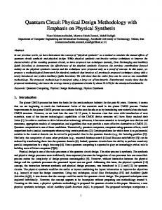
for equivalence among the resultant states and operators [26]. In the case of stabilizer circuits, we used the equivalence-checking method described in [1], [11]. Stabilizer circuits. We compared the runtime performance of single-threaded Quipu against that of CHP using a benchmark set similar to the one used in [1]. We generated random stabilizer circuits on n qubits, for n ∈ {100, 200, . . . , 1500}. The use of randomly generated benchmarks is justified for our experiments because (i) our algorithms are not explicitly sensitive to circuit topology and (ii) random stabilizer circuits have been considered representative [16]. For each n, we generated the circuits as follows: fix a parameter β > 0; then choose βdn log2 ne random unitary gates (CNOT, P or H) each with probability 1/3. Then measure each qubit a ∈ {0, . . . , n − 1} in sequence. We measured the number of seconds needed to simulate the entire circuit. The entire procedure was repeated for β ranging from 0.6 to 1.2 in increments of 0.1. Figure 9 shows the average time needed by Quipu and CHP to simulate this benchmark set. The purpose of this comparison is to evaluate the overhead of supporting generic circuit simulation in Quipu. Since CHP is specialized to stabilizer circuits, we do not expect Quipu to be faster. When β = 0.6, the simulation time appears to grow roughly linearly in n for both simulators. However, when the number of unitary gates is doubled (β = 1.2), the runtime of both simulators grows roughly quadratically. Therefore, the performance of both simulators depends strongly on the circuit being simulated. Although Quipu is 5× slower than CHP, we note that Quipu maintains global phases whereas CHP does not. Nonetheless, Figure 9 shows that Quipu is asymptotically as fast as CHP when simulating stabilizer circuits that contain a linear number of measurements. The multithreaded speedup in Quipu for non-Clifford circuits is not readily available for stabilizer circuits. Ripple-carry adders. Our second benchmark set consists of n-bit ripple-carry (Cuccaro) adder [7] circuits, which often appear as components in many arithmetic circuits [18]. The Cuccaro circuit for n = 3 is shown in Figure 10. Such circuits act on two n-qubit input registers, one ancilla qubit and one carry qubit for a total of 2(n + 1) qubits. We applied H gates to all 2n input qubits in order to simulate addition on a superposition of 22n computational-basis states. Figure 11 shows the average runtime needed to simulate this benchmark set using Quipu. For comparison, we ran the same benchmarks on an optimized version of QuIDDPro, called QPLite11 , specific to circuit simulation [26]. When n < 15, QPLite is faster than Quipu because the QuIDD representing the state vector remains compact during simulation. However, for n > 15, the compactness of the QuIDD is considerably reduced, and the majority of QPLite’s 11. QPLite is up to 4× faster since it removes overhead related to QuIDDPro’s interpreted front-end for quantum programming.
11
Fig. 7. Example simulation flow for a small non-Clifford circuit (top left) using Quipu. The multiframes obtained are pairwise orthogonal and thus no orthogonalization is required. runtime is spent in non-local pointer-chasing and memory (de)allocation. Thus, QPLite fails to scale on such benchmarks and one observes an exponential increase in runtime. Memory usage for both Quipu and QPLite was nearly unchanged for these benchmarks. Quipu consumed 4.7MB on average while QPLite consumed almost twice as much (8.5MB). We ran the same benchmarks using single and multi-
template auto async_launch( Func f, const Iter begin, const Iter end, Params... p ) -> vector< decltype( async(f, begin, end, p...) ) > { vector< decltype( async(f, begin, end, p...) ) > futures; int size = distance(begin, end); int n = size/MTHREAD; futures.reserve(MTHREAD); for(int i = 0; i < MTHREAD; i++) { Iter first = begin + i*n; Iter last = (i < MTHREAD - 1) ? begin + (i+1)*n : end; futures.push_back( async( f, first, last, p...) ); } return futures; }
H
•
•
|a0 i |0i |b1 i
H
•
•
|a1 i
H
|b2 i
H
|a2 i |zi
H
|b0 i
• •
H • •
|s0 i •
|a0 i |0i |s1 i
• •
|a1 i
• • • • • •
•
|s2 i
• •
•
•
|a2 i |z ⊕ s3 i
Fig. 10. Ripple-carry (Cuccaro) adder for 3-bit numbers a = a0 a1 a2 and b = b0 b1 b2 [7, Figure 6]. The third qubit from the top is an ancilla and the z qubit is the carry. The b-register is overwritten with the result s0 s1 s2 .
frames. The number of states in the superposition grows exponentially in n for a single frame, but linearly in n when multiple frames are allowed. This is because T OF gates produce large equal superpositions that are effectively compressed by our coalescing technique. Since our frame-based algorithms require poly(k) time for k states in a superposition, Quipu simulates Cuccaro
Fig. 8. Our C++11 template function for parallel execution of the frame operations described in Section 4.
15
10
100 β = .6 β = .7 β = .8 β = .9 β= 1.0 β= 1.1 β = 1.2
CHP
60 40
5
0 200
80
β = .6 β = .7 β = .8 β = .9 β= 1.0 β= 1.1 β = 1.2
Quipu
20
400
600
800
0 1000 1200 1400 1600 200
Runtime (secs)
Avg. Runtime (secs)
80 20
QPLite
70 60
5
Quipu
50 zoomed-in
40 30 0
20
10
15
10 400
600
800 1000 1200 1400 1600
Number of qubits
Fig. 9. Average time needed by Quipu and CHP to simulate an n-qubit stabilizer circuit with βn log n gates and n measurements. Quipu is asymptotically as fast as CHP but is not limited to stabilizer circuits.
Quadratic fit
0 5
10
15
20
25
n-bit Cuccaro adder (2n + 2 qubits)
Fig. 11. Average runtime and memory needed by Quipu and QuIDDPro to simulate n-bit Cuccaro adders on an equal superposition of all computational basis states.
Quantum Fourier transform (QFT) circuits. Our third benchmark set consists of circuits that implement the nqubit QFT, which computes the discrete Fourier transform of the amplitudes in the input quantum state. Let |x1 x2 . . . xn i, xi P ∈ {0, 1} be a computational-basis state m and x1,2,...,m = k=1 xk 2−k . The action of the QFT on this input state can be expressed as:
400
Runtime (secs)
circuits in polynomial time and space for input states consisting of large superpositions of basis states. On such instances, known linear-algebraic simulation techniques (e.g., QuIDDPro) take exponential time while Quipu’s runtime grows quadratically (best quadratic fit f (x) = 0.5248x2 − 15.815x + 123.86 with R2 = .9986). The work in [18] describes additional quantum arithmetic circuits that are based on Cuccaro adders (e.g., subtractors, conditional adders, comparators). We used Quipu to simulate such circuits and observed similar runtime performance as that shown in Figure 11.
Peak memory (MB)
12
350 300
QPLite
Quipu
250 200 150
QuipuMT
100 50 0 10
12
14
16
18
20
22
24
700 600
QPLite
Quipu
500 400 300 200
QuipuMT
100 0 10
12
14
16
18
20
22
24
n-qubit QFT circuit
Fig. 13. Average runtime and memory needed by Quipu (single and multi-threaded) and QuIDDPro to simulate nqubit QFT circuits, which contain n(n + 1)/2 gates. We used the |11 . . . 1i input state for all benchmarks.
plex amplitudes. Such non-compact data structures can be streamlined to simulate most quantum gates (e. g., Hadamard, controlled-R(α)) with limited runtime overhead, but scale to only around 30 qubits due to poor � � � 1 � 2iπ·xn−1,n 2iπ·xn memory scaling. Our results showed that Quipu was |1i ⊗ |1i ⊗ |0i + e |0i + e |x1 . . . xn i = √ 2n approximately 3× slower than an array-based imple� � 2iπ·x1,2,...,n mentation when simulating QFT instances. However, · · · ⊗ |0i + e |1i (4) such implementations cannot take advantage of circuit The QFT is used in many quantum algorithms, notably structure and, unlike Quipu and QPLite, do not scale to Shor’s factoring and discrete logarithm algorithms. Such instances of stabilizer and arithmetic circuits with > 30 circuits are composed of a network of Hadamard and qubits (Figures 9 and 11). controlled-R(α) gates, where α = π/2k and k is the distance over which the gate acts. The three-qubit QFT Fault-tolerant (FT) circuits. Our next benchmark set circuit is shown in Figure 12. In general, the first qubit consists of circuits that, in addition to preparing encoded requires one Hadamard gate, the next qubit requires a quantum states, implement procedures for performing Hadamard and a controlled-R(α) gate, and each follow- FT quantum operations [9], [19], [23]. FT operations limit ing qubit requires an additional controlled-R(α) gate. the propagation errors from one qubit in a QECC-register Summing up the number of gates gives O(n2 ) for an (the block of qubits that encodes a logical qubit) to n-qubit QFT circuit. Figure 13 shows average runtime another qubit in the same register, and a single faulty and memory usage for both Quipu and QPLite on QFT gate damages at most one qubit in each register. One instances for n = {10, 12, . . . , 20}. Quipu runs approx- constructs FT stabilizer circuits by executing each Clifimately 10× faster than QPLite on average and con- ford gate transversally12 across QECC-registers as shown sumes about 96% less memory. For these benchmarks, in Figure 14. Non-Clifford gates need to be implemented we observed that the number of states in our multiframe using a FT architecture that often requires ancilla qubits, data structure was 2n−1 . This is because controlled-R(α) measurements and correction procedures conditioned on gates produce biased superpositions (Section 4) that measurement outcomes. Figure 15 shows a circuit that cannot be effectively compressed using our coalescing implements a FT-Toffoli operation [23]. Each line repreprocedure. Therefore, as Figure 13 shows, the runtime sents a 5-qubit register based on the DiVincenzo/Shor13 and memory requirements of both Quipu and QPLite code, and each gate is applied transversally. The state � � √ grow exponentially in n for QFT instances. However, |cati = ( 0⊗5 + 1⊗5 )/ 2 is obtained using a stabilizer Quipu scales to 24-qubit instances while QPLite scales subcircuit (not shown). The arrows point to the set of to only 18 qubits. The multi-threaded version of Quipu gates that is applied if the measurement outcome is exhibited roughly a 2× speedup and used a comparable 1; no action is taken otherwise. Controlled-Z gates are amount of memory on a four-core Xeon server. implemented as Hj CN OTi,j Hj with control i and target We compared Quipu to a straightforward implemen- j. Z gates are implemented as P 2 . tation of the state-vector model using an array of comWe implemented FT benchmarks for the half-adder and full-adder circuits (Figure 16) as well as for computing f (x) = bx mod 15. Each circuit from Figure 17 • • |x2 i |y0 i H implements f (x) with a particular coprime base value •
|x1 i
|x0 i
H
R(π/2)
R(π/2)
H R(π/4)
Fig. 12. The three-qubit QFT circuit.
|y1 i
|y2 i
12. In a transversal operation, the ith qubit in each QECC-register interacts only with the ith qubit of other QECC-registers [12], [19], [23]. 13. The DiVincenzo/Shor 5-qubit code functions successfully in the presence of both bit-flip and phase-flip errors even if they occur during correction procedures [9].
13
TABLE 3 Average time and memory needed by Quipu and QPLite to simulate several quantum FT circuits. The second column shows the QECC used to encode k logical qubits into n physical qubits. Benchmarks with (∗ ) use the 5-qubit DiVincenzo/Shor code [9] instead of the 3-qubit bit-flip code. We used the |00 . . . 0i input state for all benchmarks. The top numbers from each row correspond to direct simulation of Toffoli gates (Section 4) and the bottom numbers correspond to simulation via the decomposition from Figure 18. Shaded rows are Clifford circuits for mod-exp. FAULT- TOLERANT CIRCUIT
NUM . QUBITS
QECC
[n, k]
toffoli∗
[15, 3]
45
halfadd∗
[15, 3]
45
fulladd∗
[20, 4]
80
2x mod15
[18, 6]
81
4x mod15∗
[30, 6]
30
7x mod15
[18, 6]
81
8x mod15
[18, 6]
81
11x mod15∗
[30, 6]
30
[18, 6]
81
[30, 6]
30
13x mod15 14x mod15∗
|xi
|yi
•
H
|xi
|yi
P
(a) Logical operation
CLIFF
H
H
P
P
NUM . GATES & MEAS . NON - CLIFF . 155 15 305 90 160 15 310 90 320 30 620 180 396 36 756 216 30 0 402 36 762 216 399 36 759 216 25 0 399 36 759 216 40 0
• •
H
•
P
(b) Transversal execution
Fig. 14. Transversal implementation of a stabilizer circuit acting on three-qubit QECC registers. |0i |0i |0i |cati |cati |cati |xi |yi |zi
H
r
r
r
H
r
r
r
H
r
r
e ee
e e
Z e
r
e e
H
r r
e e
H H
r
r
r
e
|xi |yi e |z ⊕ xyi
e r
Z e 6 6 6 Meas.
r
RUNTIME ( SECS )
QPLite 43.68 72.45 43.80 75.05 84.96 1173.48 4.81hrs > 24hrs 0.01 11.25hrs > 24hrs 11.37hrs > 24hrs 0.02 11.28hrs > 24hrs 0.02
Quipu 0.20 0.83 0.20 0.84 0.88 1.61 1.48 6.08 < 0.01 1.52 4.98 1.52 6.08 < 0.01 1.56 4.64 < 0.01
MEMORY
QPLite 98.45 137.02 94.82 137.03 91.86 139.44 11.85 118.17 6.14 12.41 134.05 12.48 135.18 6.14 11.85 135.23 6.14
(MB) Quipu 12.76 12.78 12.76 12.78 12.94 13.52 12.96 14.23 12.01 13.29 14.77 13.29 14.77 12.01 12.25 14.62 12.01
MAX SIZE (Ψ) SINGLE F MULTI
2816 8192 2816 8192 2816 16384 22528 222 1 22528 222 22528 222 1 22528 222 1
F
32 32 32 32 32 32 64 64 1 64 64 64 64 1 64 64 1
more robust 5-qubit code in our larger benchmarks. Our results in Table 3 show that Quipu is typically faster than QPLite by several orders of magnitude and consumes 8× less memory for the toffoli, half-adder and full-adder benchmarks. For FT benchmarks that consist of stabilizer circuits (shaded rows), the QuIDD representation remains compact and utilizes half as much memory as our frame representation. Table 3 also shows that our coalescing technique is very effective as the maximum size of the stabilizer-state superposition is much smaller when multiple frames are used. Since the total number of states observed is relatively small, the multithreaded version of Quipu exhibited similar runtime and memory requirements for these benchmarks.
Meas.
r
Meas.
e
Meas.
e
Meas.
r H
Meas.
Fig. 15. Fault-tolerant implementation of a Toffoli gate. b as a (2, 4) look-up table (LUT).14 The Toffoli gates in all our FT benchmarks are implemented using the architecture from Figure 15. Since FT-Toffoli operations require 6 ancilla registers, a circuit that implements t FT-Toffolis using a k-qubit QECC, requires 6tk ancilla qubits. Therefore, to compare with QPLite, we used the 3-qubit bit-flip code [19, Ch. 10] instead of the 14. A (k, m)-LUT takes k read-only input bits and m > log2 k ancilla bits. For each 2k input combination, an LUT produces a pre-determined m-bit value, e.g., a (2, 4)-LUT is defined by values (1, 2, 4, 8) or (1, 4, 1, 4).
Technology-dependent circuits. Section 4 outlines how Quipu supports primitive gate libraries, especially for quantum-optical systems where Clifford gates are considered primitive [17]. Therefore, to simulate FT circuits for photonic systems, it suffices to decompose T OF F gates into sequences of Hadamard, CNOT and T gates as shown in Figure 18. Table 3 reports simulations of our FT benchmarks using such decompositions. Since the total number of gates is larger, Quipu is roughly
|xi |yi |0i
• •
•
|xi |sumi
|ai |bi |zi
|carryi
|0i
(a) Half adder
• • •
•
• •
|xi |yi |sumi |carryi
(b) Full adder
Fig. 16. Adder circuits implemented in our benchmarks.
14
|x0 i
H
|x1 i
H
•
•
H
• •
H
•
•
H H
•
•
H
•
•
H
• •
•
|x0 i |x1 i
|0i
|y0 i
|0i
|y1 i
|0i
|y2 i |y3 i
|0i b=2
b=4
b=7
b=8
Fig. 17. Mod-exp with M = 15 implemented as (2, 4)LUTs [18] for several coprime base values. Negative controls are shown with hollow circles. 4× slower as compared to direct simulation of T OF F gates. QPLite takes > 24 hours to simulate several of these benchmarks while Quipu takes only several seconds since the majority of the gates introduced by the decomposition from Figure 18 are Clifford gates.
7
new Clifford miters – linear combinations of Clifford operators that represent a specific quantum circuit. Clifford miters can speed up formal verification by exploiting similarities in circuits and the fast equivalence-checking algorithms from [1], [11]. Section 4 described how Quipu incorporates quantum machine descriptions in the form of primitive gate libraries to simulate technology-dependent circuits. This method can benefit from new decompositions for library gates into linear combinations of Pauli or Clifford operators. Such decompositions can be obtained on the fly when simulating original gates one-by-one in sequence. They can also be precomputed and used for a compiled version of the original circuit, where scheduling can be optimized for parallelism and architecture constraints. Acknowledgements. This work was sponsored in part by the Air Force Research Laboratory under agreement FA8750-11-2-0043.
C ONCLUSIONS
In this work, we developed new techniques for quantum-circuit simulation based on superpositions of stabilizer states, avoiding shortcomings in prior work [1]. To represent such superpositions compactly, we designed a new data structure called a stabilizer frame. We implemented stabilizer frames and relevant algorithms in our software package Quipu. Current simulators based on the stabilizer formalism, such as CHP, are limited to simulation of stabilizer circuits. Our results show that Quipu performs asymptotically as fast as CHP on stabilizer circuits with a linear number of measurement gates, but simulates certain quantum arithmetic circuits in polynomial time and space for input states consisting of equal superpositions of computational-basis states. In contrast, QuIDDPro takes exponential time on such instances. We simulated quantum Fourier transform and quantum fault-tolerant circuits with Quipu, and the results demonstrate that our stabilizer-based technique leads to orders-of-magnitude improvement in runtime and memory as compared to QuIDDPro. While our technique uses more sophisticated mathematics and quantum-state modeling, it is significantly easier to implement and optimize. In particular, our multithreaded implementation of Quipu exhibited a 2× speed up on a four-core server. Future Directions. The work in [27] describes an equivalence-checking method for quantum circuits based on the notion of a reversible miter – a counterpart of miter circuits used in equivalence-checking of digital circuits. An attractive direction for future work is deriving
R EFERENCES [1] [2] [3] [4] [5] [6] [7] [8] [9] [10] [11] [12] [13] [14] [15] [16] [17] [18] [19]
• •
•
•
•
≡ H
• T†
T
• T†
T†
T
• T†
T P
H
Fig. 18. The Toffoli gate and its decomposition into onequbit and CNOT gates [19, Figure 4.9].
[20] [21] [22] [23]
S. Aaronson, D. Gottesman, “Improved Simulation of Stabilizer Circuits,” Phys. Rev. A, vol. 70, no. 052328 (2004). D. Aharonov. “A Simple Proof that Toffoli and Hadamard are Quantum Universal,” arXiv:0301040 (2003). K. M. R. Audenaert, M. B. Plenio, “Entanglement on Mixed Stabilizer States: Normal Forms and Reduction Procedures,” New J. Phys., vol. 7, no. 170 (2005). A. Barenco et al., “Approximate Quantum Fourier Transform and Decoherence,” Phys. Rev. A, vol. 54, pp. 139–146 (1996). O. Boncalo et al., “Using Simulated Fault Injection for Fault Tolerance Assessment of Quantum Circuits,” Proc. Sim. Symp., pp. 213–220 (2007). D. Coppersmith, “An Approximate Fourier Transform Useful in Quantum Factoring,” arXiv:0201067 (2002). S. A. Cuccaro et al., “A New Quantum Ripple-carry Addition Circuit,” arXiv:0410184v1 (2004). K. De Raedt et al., “Massively Parallel Quantum Computer Simulator”, Comp. Phys. Comm., vol. 176, no. 2 (2007). D. P. DiVincenzo, P. W. Shor, “Fault-Tolerant Error Correction with Efficient Quantum Codes”, Phys. Rev. Lett., vol. 77, no. 3260 (1996). I. Djordjevic, Quantum Information Processing and Quantum Error Correction: an Engineering Approach, Academic press (2012). H. J. Garcia, I. L. Markov, A. W. Cross, “On the Geometry of Stabilizer States,” Quant. Info. and Comp., vol. 14, no. 7–8 (2014). D. Gottesman, “The Heisenberg Representation of Quantum Computers,” arXiv:9807006v1 (1998). L. Grover, “A Fast Quantum Mechanical Algorithm for Database Search,” Symp. on Theory of Comp., pp. 212–219 (1996). T. W. Hungerford, Algrebra, Springer (1974). N. Isailovic et al., “Interconnection Networks for Scalable Quantum Computers,” Inter. Symp. on Comp. Arch., pp. 366–377 (2006). E. Knill et al., “Randomized Benchmarking of Quantum Gates,” Phys. Rev. A., vol. 77, no. 1 (2007). C. Lin, A. Chakrabarti, N.K. Jha, “Optimized Quantum Gate Library for Various Physical Machine Descriptions,” IEEE Trans. on VLSI Sys., vol. 21, no. 11 (2013). I. L. Markov, M. Saeedi, “Constant-optimized Quantum circuits for Modular Multiplication and Exponentiation,” Quant. Info. and Comp., vol. 12, no. 5 (2012). M. A. Nielsen, I. L. Chuang, Quantum Computation and Quantum Information, Cambridge University Press (2000). K. M. Obenland, A. M. Despain, “A Parallel Quantum Computer Simulator, ” arXiv:9804039 (1998). B. Oemer, http://tph.tuwien.ac.at/∼oemer/qcl.html (2003). M. Oskin, F. T. Chong, I L. Chuang, “A Practical Architecture for Reliable Quantum Computers,” IEEE Computer, vol. 35, no. 1 (2002). J. Preskill, “Fault Tolerant Quantum Computation,” Introduction to Quantum Computation, World Scientific (1998). arXiv:9712048.
15
[24] P. Shor, “Polynomial-time Algorithms for Prime Factorization and Discrete Logarithms on a Quantum Computer,” SIAM J. Comput, vol. 26, no. 5 (1997). [25] K. M. Svore, A. V. Aho, A. W. Cross, I. L. Chuang, I. L. Markov, “A Layered Software Architecture for Quantum Computing Design Tools,” IEEE Computer, vol. 39, no. 1 (2006). [26] G. F. Viamontes, I. L. Markov, J. P. Hayes, Quantum Circuit Simulation, Springer (2009). [27] S. Yamashita, I. L. Markov, “Fast Equivalence-checking for Quantum Circuits” Quant. Info. and Comp., vol. 9, no. 9–10 (2010).