SIMULATION OF RAIN EVENTS TIME SERIES WITH MARKOV MODEL Clémence Alasseur1, Lionel Husson1, Fernando Pérez-Fontán2 1 2
Supélec, 3 rue Joliot-Curie, 91192 Gif-sur-Yvette, France,
[email protected],
[email protected] Universidad de Vigo ETSE Telecomunicación, Campus Universitario, E-36200, Vigo, Spain,
[email protected]
Abstract – This paper presents a rain rate time series model based on a two-level Markov model structure. ‘Rain’ or ‘No-Rain’ events are generated in two steps: in a first time, the ‘Rain’ or ‘Inter-Rain’ duration of the considered event is determined according to the experimental data series. This corresponds to the first level of the model that is a semi-Markov model. In a second time, the rain rate intensities are generated resorting to a N states Hidden Markov Model based on the conditional probabilities of experimental rain samples (modeling the dependence of the current rain intensity with the previous one). This two-level model produces simulated rain samples whose statistics fit very accurately those of the experimental data without using any stored rain events in the generation step when the model is known. Keywords – rain modeling, Markov model, satellite channel I. INTRODUCTION Nowadays, satellite communications systems need to operate to higher frequency bands like the Ka or V bands because of the congestion at lower bands. To these high frequencies, rain events cause severe attenuation to the propagation channel and then accurate modelling of their effects will enable to conteract them efficiently through adapted Fade Mitigation Techniques (FMTs). As rain attenuation is strongly correlated with rain rate intensity, modeling of rain rate time series is then interesting for satellite communications at high frequencies. This paper presents a new rain rate model that is based on a Markov chain structure [1,2,3] and that uses the dependency of one rain rate sample with its previous time sample. To account of this particularity, the chosen Markov structure is a two-level model. The first level models the ‘Rain’ and ‘Inter-Rain’ (or no rain) states; the first level is in reality a semi-Markov chain which accounts for the particular duration distributions of these two states. The second level is directly linked to the rain state, it is a basic N-state Markov chain that models the rain rate intensity by taking into account the previous sample. This paper is divided into four parts: the first one presents the adopted model for rain rate time series generation. The two following parts justify the choice of the form of the
model: part three explains the choice of a semi-Markov model for the first level of the model by giving the ‘Rain’ and ‘Inter-Rain’ duration distributions. And part four presents the conditional distributions of the rain rates which lead to the Markov chain of the second level of the model. Next, part five gives the main results and compares the statistics of the experimental and generated rain rate time series. II. MODEL A Hidden Markov Model (HMM) [4] is a model composed of N states, where the probability to have a particular state at time (t+1) is only dependent on the state at time t. An HMM is composed not only of the state sequence but also of an observation sequence. The observations, in the considered application, are the rain rate levels, and are available to the observer whereas the state sequence is hidden or unknown. In fact, one model state corresponds to a particular distribution from which the observation is generated when the system is in this state. The adopted model consists of two-level Markov chain. The first level is a semi-Markov chain of two states: ‘rain’ and ‘inter-rain’. A semi-Markov is used to enable every possible duration distribution for rain and inter-rain events,
rain
inter-rain
pkk k
pNk pkN
N pNN
pN1
p1N
P2k p22 p1k
pk2
pk
p12 1
2
p21
p11
Fig 1: global two level Hidden Markov model
III. RAIN AND INTER-RAIN DURATION The rain and inter-rain duration distributions can not be modeled by a simple Markov model. In fact, Markov model imposed the state duration to be issued from an exponential law. In a Markov chain, the probability that the model stays in the particular state i for a duration of d
samples is equal to: f i (d ) = p ii d −1 (1 − p ii ) with p ii the probability to remain in state i during two consecutive samples. The transition probability p ii for state ‘Rain’ and ‘Inter-Rain’ are calculated from the experimental data and are presented in table1. Table1: Markov probability to remain in one state Prain − rain
0.8810
Pinter⋅rain −inter⋅rain
0.9916
The two next figures are the illustration of the rain and inter-rain duration distribution (in blue) and of the exponential distribution f i (d) induced by the Markov model (in dashed red). Table 1 presents the probability to stay in rain or in inter-rain state for a time sample of approximatively 5 min. The exponential distributions of fig. 1 and 2 are using these parameters. 0.25
probabiltiy distribution
0.3
0.2 0.15 0.1 0.05 0 0
100
200
300
400
500
600
Rain and inter-rain duration distributions can clearly not be modeled by this type of law. This is the reason why we resort to a semi-Markov model [4]. A semi-Markov model can adopt any suitable duration distribution. In the following, the state durations (‘Rain’ and ‘Inter-Rain’ durations) are sampled from the experimental duration distributions obtained from the experimental rain rate time series. No attempt to fit theoretical distributions on these distributions is made. IV. RAIN RATE DISTRIBUTION A. Rain distribution The rain rate time series has been measured in Santiago de Compostela airport in Spain for a total duration of approximatively 10 years. The time interval between two consecutive samples is roughly 5 minutes and rain rates are measured in mm/h. Fig. 4 shows a small time interval of the experimental time series. 40 35 30 25 20 15 10 5 0 0.9
probabiltiy distribution
inter-rain duration distribution Markov duration distribution
0.25
inter-rain event duration (×5min) Fig. 3: inter-rain event duration distribution
rain rate (mm/h)
and the duration of each state is linked to distributions detailed in part two. When the system is in the rain state, rain rate levels are generated through a Markov chain of N states that is the second level of the global model. Thus, rain samples are assumed to be dependent only on the previous rain sample. When the model is in the inter-rain state, we can consider that it generates null rain rate samples: no additive Markov chain is required for the inter-rain state. Fig. 1 shows the global model: the twostate semi-Markov model with the ‘Rain’ and ‘Inter-Rain’ state, the link from the rain state to the N state Markov chain, every states of this chain are linked to the others with different transition probability p ik from state i to state k.
1
1.1
1.2
1.3
1.4
1.5
1.6
1.7
time sample/5mm x 10 Fig. 4: example of experimental rain rate time series 4
0.2 rain duration distribution Markov duration distribution
0.15
As stated in [5], the distribution of the rain rate can be fitted to a lognormal distribution. Next figure illustrates the superposition of the rain distribution estimated on the experimental rain rate time series with the fitted lognormal distribution.
0.1
0.05
0 0
10
20
30
40
50
60
70
80
rain event duration (×5min) Fig. 2: rain event duration distribution
0
10
-1
10
-2
10
-3
10
-4
10
-5
10
-6
10
-7
-8
10 -1 10
Each conditional distribution of log of rain rates can be associated to a Gaussian distribution. The two next figures are the evolution of the mean and of the variance of the Gaussian distribution parameters for each conditional probability. On these figures, the number of considered conditional probability is 42 because it is the number of states that will be considered in the following. On fig. 6 only 5 conditional distributions are represented in order not to alter the figure. We observe that the mean (fig. 7) is linearly increasing and the variance (fig. 8) can be roughly assimilated to the square curve.
experimental distribution lognormale distribution 10
0
10
1
10
2
10
3
rain rate (mm/h) Fig. 5: experimental and theoretical lognormal inverse cumulative distribution
2.5
conditional distribution mean
rain rate distribution
10
2
1.5 1
0.5
B. Conditional distributions To take account of the influence of the previous rain rate sample, we have to extract the distribution of the rain rate sample when the previous sample is known. If the Markov model of the rain rate is composed of N states, the observation intervals (rate i )1≤i ≤ N are set in such
a way that the probability to belong to the interval [rate i , rate i +1 ] is constant whatever the value of index i. We thus obtain N conditional probabilities of observing rain rate x at time t knowing that at time (t-1) the rain rate was in the ith observation interval P(x (t ) rate i ≤ x (t − 1) ≤ rate i +1 ) . It should be notice that the conditional probabilities are calculated onto the log of the rain rates because their shape was much easier to fit to theoretical distributions.
rain rate conditional distribution
Fig. 6 shows examples of the conditional probability according to five observation intervals. 0.09
0
-0.5 -1
-1.5 0
5
10
observation interval number 15
20
25
30
35
40
45
Fig. 7: the conditional distribution P(x (t ) x (t − 1)) mean conditional distribution variance
But generating rain rate directly from the corresponding log normal distribution does not produce good results. In fact, rain rate samples are dependent on previous ones [1,6]. That why conditional probabilities have to be considered to model accurately the rain rate time series.
0.9
0.85 0.8
0.75 0.7
0.65 0.6
0.55 0
5
10
15
20
25
30
35
40
45
observation interval number Fig. 8: conditional distribution P(x (t ) x (t − 1)) variance The Gaussian parameters determine the conditional probability of observing one rain rate intensity knowing the previous rain rate. Thus, it determines the transition probability of the Markov model: to each Markov state one condition distribution or one set of Gaussian parameters (mean and variance) is associated. And each state of the second level rain Markov chain is equiprobable because of the observation intervals we considered.
0.08 0.07
V. RAIN RATE GENERATION AND RESULTS
0.06
A. Generation
0.05 0.04
A Markov chain with N=42 states is considered in the following for the generation of the rain rate time-series. We develop a method to generate the log of the rain rate according to the model presented in part two:
0.03 0.02 0.01 0 -8
-6
-4
-2
0
2
4
log of rain rate (mm/h)
6
Fig. 6: conditional distribution P(x (t ) x (t − 1))
- Init phase: determine the first state: ‘Rain’ or ‘interrain’. The probability for a sample to be in the rain state is 0.06 and to be in the inter-rain state is 0.94.
- Processing: generate the current state (‘Rain’ or ‘inter-rain’) duration d according to the corresponding duration distribution (fig. 2 and 3)
probabiltiy distribution
0.2 experimental rain duration distribution generated rain duration distribution
0.15
→ ‘Inter-Rain’ event: rain rate is null for d samples → ‘Rain’ event:
0.1
0.05
generate a first sample according to the global normal distribution of the log of the rain rate (fig. 5)
probabiltiy distribution
(d-1) times
40
return to processing step
experimental inter-rain duration distribution generation inter-rain duration distribution
0.2
0.1
0
50
100
150
10
5
0 2.4
2.42
2.44
2.46
2.48
2.5
2.52
2.54
2.56
2.58
4
16 14 12 10 8 6 4 2
0
experimental
rain rate (mm/h)
2
18
rain rate (mm/h)
4
20
distribution of the log of the rain rate
generated
20
6
1.65
1.66
400
450
1.67
1.68
1.69
1.7
1.71
1.72
1.51
1.52
1.53
1.54
1.55
1.56
time sample/5mm time sample/5mm Fig. 10: zoom on rain events x 10
4
0.02
0.015
0.01
0.005
0 -8
0 1.64
350
experimental rain rate distribuion generated rain rate distribution
x 10
8
300
0.025
2.6
time sample/5mm Fig. 9: generated rain rate time series
10
250
Then the distributions and the inverse cumulative distributions of the log of both rain rate time series are represented respectively on fig. 12 and 13. Here again, good agreement is shown between the experimental and simulated data.
15
12
200
inter-rain event duration Fig. 11: ‘Rain’ and ‘Inter-Rain’ duration distribution
20
14
100
0.05
25
16
80
0.15
30
18
60
0.3
0.25
We obtain the following rain rate time series (zoom) on fig. 9. Fig. 10 shows generated and experimental rain rate events, the generated series shows great similitude with the experimental one. rain rate (mm/h)
20
rain event duration
according to the previous sample, draw (d-1) new samples from conditional probabilities P(x (t ) x (t − 1))
0
1.57 x 10
B. Main results
In this part, we try to characterize the observed similitude in fig. 9 and 10 between the generated and experimental data. First, the ‘Rain’ and ‘Inter-Rain’ distributions are illustrated in the two following figures, they show perfect matching between the experimental and simulated sequence.
4
-6
-4
-2
0
2
4
6
log of rain rate (mm/h) Fig. 12: distribution of the log of the rain rate Here is the second-order statistic [1,7] for four different threshold levels: 0, 1, 5 and 10 mm/h. The second order statistic is the probability to have a rain event where every rain samples are superior to the threshold R and whose duration (Te − Tb ) is superior to the abscissa: PR (x , ∆t ) = P(∀t 0 ∈ [Tb , Te ], x (t 0 ) > R , and(Te − Tb ) > ∆t ) where Tb is the time index of the beginning of the event, Te of the end. The plots are shorter for the threshold of 10mm/h for example because the probability to encounter a rain event whose every sample is superior 10mm/h diminishes with the duration. The plot for the threshold 0mm/h considers all the rain events.
VI. CONCLUSIONS
inverse cumulative distribution
Every curves show very good agreement between the experimental rain time series and the generated one when the number of states is 42 (red dashed curves) and when the number of states is 7 (black dotted curves). The inverse cumulative distribution (fig. 13), when the rain is generated with N=42, fits better the experimental one than the one when the rain is generated using only 7 states. When only 7 states are considered, highest level of rain rate intensity samples are minimized compared to the experimental results. Fig. 14 is the illustration of the second order statistics for the experimental data, the data generated with 42 states, and the data generated with 7 states. Here again, the results are better for 42 states than for 7. For low thresholds, 0 and 1 mm/h, the curves do not present differences but as soon as the threshold increases, 5 and 10mm/h, the curve for 7 states presents erroneous probabilities to obtain long events whose every samples are superior to the threshold. Hence, to take a larger HMM (42 states rather than 7) enables to fit better high intensity events. 10
0
10
-1
10
-2
10
-3
10
-4
10
-5
-8
We propose in this paper an original model of rain rate intensities. It is based on a two-level Markov models. The first level is a two-state semi-Markov model (‘Rain’ and ‘Inter-Rain’ states) where the state duration distributions are determined to fit the experimental data sets. The second level of the model is an HMM based on the conditional probability of the rain samples. This model produces accurate rain rate time series whose statistics match accurately the experimental rain rate statistics. Some possible improvements would be to take into account the particularity of the first and last rain samples. Furthermore, a relevant criterion for the automatic determination of the optimal number of states of the second level HMM could be specified. ACKNOWLEDGEMENTS The rain rate database used in this study was supplied by the Radiocommunications Group at the Polytechnic University of Madrid. REFERENCES [1]
[2] experimental rain rate distribution simulated with N=7 simulated with N=42 -6
-4
-2
0
2
4
[3]
6
log of rain rate
Fig. 13: inverse cumulative distribution of the log rain rate 10
10
10
threshold = 0 mm/h
0
10
-1
[5] -2
rain event duration 5min/sample
10
10
[4]
threshold = 1 mm/h
0
10
0
threshold = 5 mm/h
0
10
10 -2
10
-2
10
-3
10
-4
10
-4
10
-6
rain event duration 5min/sample
10
0
10
1
10
[6]
rain event duration 5min/sample
-5
0
10
1
10
threshold = 10 mm/h
[7]
-5 rain event duration 5min/sample
1
Fig. 14: second order statistics for four thresholds
2
4
F. Pérez-Fontan, U.-C. Fiebig, C. Enjamio. L. Husson, A. Benarroch, “Synthetic rain-rate time-series generation for radio system Simulation”, ClimDiff, Nov 2003. U.-C. Fiebig, F. Pérez-Fontán: "First Results on Modeling Rain Rates", 4th COST-280 Meeting, Prague, Czech Republic, 2002. U.-C. Fiebig, "A Time-Series Generator Modelling Rain Fading and its Seasonal and Diurnal Variations", 1st International Workshop of COST-Action 280, Malvern, UK, 2002. R. Rabiner, “a Tutorial on Hidden Markov Models and Selected Applications in Speech Recognition”, proceedings of the IEEE, vol. 77, no. 2, February 1989, pp. 257-286 K. S. Paulson, “The spatial-temporal statistics of rain rate random fields”, Radio Science, vol. 37, no. 5, pp. 21-1:21-8, Sept. 2002 M.M.J.L. van de Kamp, “Rain Attenuation as a Markov Process: The Meaning of two samples”, COST 280, 1st International Workshop, July 2002 F. Pérez-Fontan, U.-C. Fiebig, C. Enjamio. L. Husson, A.I. Castro, «Improving Rain Rate Time-Series Generation for System Simulation Applications», 5th MCM May 2003.