Christopher B. Cook. Marshall C. Richmond ..... applications from neutrally buoyant flow tracers (e.g. a stream of Rhodamine dye injected into the flow) to air ...
U.S. ARMY CORPS OF ENGINEERS PORTLAND DISTRICT
SIMULATION OF TAILRACE HYDRODYNAMICS USING COMPUTATIONAL FLUID DYNAMICS MODELS
Final Report
Christopher B. Cook Marshall C. Richmond
May 2001
Prepared by: Pacific Northwest National Laboratory P.O. Box 999 Richland, WA 99352 Report Number: PNNL-13467
iii
Acknowledgements We would like to acknowledge the U.S. Army Corps of Engineers for supporting this work through the High Flow Outfalls Project, Anadromous Fish Evaluation Program, FY2000 study codes SBE-P-00-10 and SBE-P-00-11. In particular, the authors would like to thank Laurie Ebner and Bob Buchholz, Portland District USACE, for their input and comments.
Pacific Northwest National Laboratory
April 2001
iv
Table of Contents ACKNOWLEDGEMENTS ....................................................................................................iii 1
BACKGROUND AND MOTIVATION ......................................................................... 1
2 MODELS CAPABLE OF SIMULATING RAPIDLY VARIED FREE-SURFACE FLOW ........................................................................................................................................ 4 2.1. 2.2. 2.3. 2.4. 3
FLOW-3D................................................................................................................... 4 STAR-CD ................................................................................................................... 5 FLUENT ..................................................................................................................... 6 MODEL SELECTION: VOF VERSUS MODIFIED VOF ..................................................... 6
VERIFICATION OF THE FREE-SURFACE HYDRODYNAMIC MODEL........... 8 3.1. 3.2. 3.3.
HYDRAULIC JUMP ........................................................................................................ 8 DROP STRUCTURE ....................................................................................................... 9 JOHN DAY SPILLWAY ................................................................................................ 11
4 APPLICATION TO THE BONNEVILLE SECOND POWERHOUSE OUTFALL AND TAILRACE ................................................................................................................... 14 4.1. 4.2. 4.3. 4.4. 4.5.
SKIMMING OUTFALL: COMPARISON TO 1:30 SCALE MODEL ...................................... 14 CANTILEVER OUTFALL: COMPARISON TO 1:30 SCALE MODEL................................... 19 PROTOTYPE: DEVELOPMENT OF BATHYMETRIC DATA ............................................... 22 PROTOTYPE OUTFALL AND TAILRACE: OCTOBER 3, 2000......................................... 24 PROTOTYPE TAILRACE: FEBRUARY 7, 2000. COMPARISON TO ADCP....................... 27
5
FULL TAILRACE MODEL ......................................................................................... 30
6
CONCLUSIONS ............................................................................................................. 31
7
FUTURE APPLICATIONS........................................................................................... 32
REFERENCES ....................................................................................................................... 34
Table of Figures Figure 1 Aerial view of Bonneville Project................................................................................ 2 Figure 2 Aerial View of the Second Powerhouse at Bonneville Project.................................... 3 Figure 3 The numerical solution at pseudo-steady state, contoured by velocity magnitude...... 8 Figure 4 Comparison between observed and simulated (FLOW-3D) water-surface elevations.9 Figure 5 Schematic diagram of the drop structure test case ....................................................... 9 Figure 6 Numerical solution (FLOW-3D) of the Drop Structure test case. ............................. 10 Figure 7 Comparison of results for the Drop Structure test case.............................................. 10 Figure 8 Longitudinal slice through 3-D numerically modeled domain. ................................. 11 Figure 9 Physical model results................................................................................................ 12 Figure 10 FLOW-3D results along the spillway centerline – with deflector case. .................. 12 Figure 11 FLOW-3D results along the spillway centerline - no deflector case. ...................... 12 Figure 12 Skimming test case: 3-D perspective of the velocity contours (ft/s)....................... 15 Figure 13 Location of the five data cross sections sampled in the skimming case. ................. 17 Figure 14 Skimming case: plan view velocity comparison. ..................................................... 18
Pacific Northwest National Laboratory
April 2001
v
Figure 15 Skimming case: side view velocity comparison. ..................................................... 18 Figure 16 Skimming case: 3-D perspective of the velocity contours (ft/s). ............................. 19 Figure 17 Cantilever case: location of the free-falling jet. ....................................................... 20 Figure 18 Location of the five data cross sections sampled in the cantilever case. ................. 21 Figure 19 Cantilever case: plan view velocity comparison. ..................................................... 21 Figure 20 Bonneville Second Powerhouse bathymetric survey data points............................. 22 Figure 21 Tailrace bathymetry at the Bonneville Dam Second Powerhouse. .......................... 23 Figure 22 Tailrace bathymetry near the high flow outfall exit................................................. 23 Figure 23 3-D perspective of the Oct 3, 2000 prototype case simulation ................................ 24 Figure 24 Velocity ribbon through the jet centerline for the Oct 3, 2000 prototype test case . 25 Figure 25 Plan view perspective for the Oct 3, 2000 prototype test case................................. 26 Figure 26 Path of drogue released upstream of the outfall at 2500cfs. .................................... 26 Figure 27 Numerical simulation results versus observed data at +3 ft elevation. .................... 28 Figure 28 Numerical simulation results versus observed data at -6 ft elevation. ..................... 28 Figure 29 Numerical simulation results versus observed data at -14 ft elevation. ................... 29 Figure 30 Observed versus simulated results for the three elevations...................................... 29 Figure 31 STAR-CD simulation results for the entire Bonneville Project Tailrace................. 30
Table of Tables Table 1 Skimming Case: mean velocity and RMS error by cross-section ............................... 17 Table 2 Cantilever Case: mean velocity and RMS error by cross-section ............................... 21 Table 3 Mean Magnitudes and RMS Errors by Depth for Both Models.................................. 27
Pacific Northwest National Laboratory
April 2001
1
1 Background and Motivation This report investigates the feasibility of using computational fluid dynamics (CFD) tools to investigate hydrodynamic flow fields surrounding the tailrace zone downstream of hydraulic structures. Previous and ongoing studies using CFD tools to simulate gradually varied flow with multiple constituents [e.g., Richmond, et al. (2000) and Perkins and Richmond (1999)] and forebay/intake hydrodynamics [Rakowski and Richmond (2000) and Rakowski, et al. (2000)] have shown that CFD tools can provide valuable information for hydraulic and biological evaluation of fish passage near hydraulic structures. These studies however are incapable of simulating the rapidly varying flow fields that involve breakup of the free-surface, such as those typically found near outfalls and spillways. Although the use of CFD tools for these types of flows are still an active area of research, initial applications discussed in this report show that these tools are capable of simulating the primary features of these highly transient flow fields. To better understand where these types of tools may be applied, consider the hydrodynamics of the high-flow outfall at Bonneville Dam. When Bonneville Dam was constructed in the 1930’s, engineers designing the dam suspected it might have negative repercussions on anadromous fish species. It was for this reason that fish ladders and various other structural devices were designed into the Dam’s original structure. However since construction of this and other dams on the Columbia and Snake River system, the number of smolt passing through Bonneville Dam has decreased and alternative methods are being sought to create conditions better suited for migration. To improve understanding of the hydrodynamic and water quality conditions that surround Bonneville Dam, physical and numerical models of various complexities have been applied. Figure 1 shows an aerial view of the Bonneville Project. Labels have been applied to the figure indicating where different multi-dimensional hydrodynamic models might be best suited. As the models become more complex (i.e. as the number of simulated dimensions and processes increases), the number of computations required to compute a solution increases dramatically. Also, with each increase in simulated dimension the computational grid over which the fluid equations are solved becomes increasingly difficult to develop, leading to higher development costs. Therefore, in areas where gradients are small, the hydrodynamic flow field can be integrated over one or two dimensions. For the Bonneville Project, these areas are upstream and downstream of the dam where lateral and vertical variations in the hydrodynamic field are relatively small. In these regions, one-dimensional models that simulate longitudinal variations are adequate for synoptic scale management decisions. There are, of course exceptions, such as the simulation of juvenile fish movements, which may require the application of multi-dimensional models.
Pacific Northwest National Laboratory
April 2001
2
1-D or 2-D 3-D non-hydrostatic
2-D or 3-D hydrostatic
2-D or 3-D hydrostatic
1-D or 2-D Figure 1 Aerial view of Bonneville Project. Labels suggest the different multi-dimensional hydrodynamic models that might be applied to simulate the area.
Close to the Project, vertical and horizontal variations are significant, and threedimensional models are warranted. Oftentimes these models employ the hydrostatic pressure assumption (i.e. changes in pressure are linear with depth), which is valid in areas of small vertical accelerations. Around intakes, spillways, and outfall structures the assumption of small vertical accelerations is obviously not valid, and a fully three-dimensional nonhydrostatic model is necessary. In addition, when modeling high flow outfalls (or in the general case modeling freefalling jets) or flow over the spillway, breakup of the free surface is an important component of the flow field. To capture these variations, CFD tools must be capable of simulating transient oscillations and breakup (i.e. droplets and breaking waves) of the water surface or falling jet. To simulate these motions, a special class of 3-D non-hydrostatic models must be used that do not employ the “rigid-lid” approximation and are capable of simulating the fine scale turbulent motions that occur in these zones. Models capable of simulating these zones are the focus of this report.
Pacific Northwest National Laboratory
April 2001
3
3-D non-hydrostatic free-surface
3-D non-hydrostatic
3-D hydrostatic
Figure 2 Aerial View of the Second Powerhouse at Bonneville Project. Labels suggest the various threedimensional hydrodynamic models that might be applied to simulate the area. The high flow outfall area shown is in upper right corner.
The objectives of this project (which also describes the outline of this report) are: A) Chapter 2: review representative CFD tools that are capable of simulating a high flow outfall, including the downstream plunge pool. The high-flow outfall (as opposed to the spillway) was chosen because of ongoing research to develop a fish passage system using this structure at Bonneville Dam. Among the items considered are the mathematical formulation, turbulence closure approximation, air entrainment capabilities, computational efficiency, and ease of computational mesh generation and presentation of simulation results. The intent was not to perform an all-inclusive survey, but to review current state of the art CFD tools capable of simulating key elements of a high flow outfall or spillway. B) Chapter 3: verify the CFD model by simulating several well documented and peer reviewed laboratory physical models. Three cases were simulated that capture the relevant hydrodynamics of the tailrace zone and CFD results were compared to observed data, where available. For ease of comparison with the published literature, two of these test cases were reported in metric units. Except for these cases, English units have been used throughout this report. Also, for the third test case (spillway), since velocity data were not available in the tailrace pool, a graphical comparison was performed showing the tailrace flow field. C) Chapter 4: apply the CFD models at prototype scale. To demonstrate the capability of the models to simulate tailrace hydrodynamics over a large horizontal extent, the tailrace below Bonneville Dam Second Powerhouse was simulated. Although comparisons to 1:30 scale physical model observations were performed, the CFD model was based upon prototype dimensions. Comparisons were also made to velocity data observed in the field on February 7 and October 3, 2000. Pacific Northwest National Laboratory
April 2001
4
2 Models Capable of Simulating Rapidly Varied Free-Surface Flow Several CFD models that are theoretically capable of simulating the high-flow outfall area were reviewed in this project. The necessary requirements of these models are that they numerically solve the three-dimensional Navier-Stokes equations without using the hydrostatic approximation and are capable of simulating a transient free-surface. All of the models documented in this report satisfy these requirements plus are commercially available, have technical support available from the vendor, have graphical preprocessors for developing the computational mesh, export simulation results in a format compatible with popular graphical post-processors, and have a proven track record of success in related fields (many were initially developed for the aerospace and automobile industry). A survey of relevant CFD models is documented by Frietas (1995), in which authors of the CFD models simulated various laboratory test cases. This survey documents that those models listed below have the fundamental capability to simulate three-dimensional nonhydrostatic flow fields. Unfortunately this review did not test the capability of these models to simulate free-surface breakup, which was still in its infancy at that time. When the model tests were performed (1993-94), the only model capable of simulating these type of freesurface flows was FLOW-3D, one of the pioneers in this area of CFD modeling.
2.1.
FLOW-3D
FLOW-3D is a finite-difference, transient-solution program that solves the conservative form of the Navier-Stokes equations over a non-uniform Cartesian grid. The origins of the FLOW-3D model can be traced back to Los Alamos National Laboratory and the research of C. W. Hirt. Research by Hirt and others lead to creation of the SOLA-VOF, NASA-VOF, and RIPPLE programs, which are documented in several publications (Nichols, et al. 1980; Hirt and Nichols, 1981; Torrey, et al. 1987; Kothe, et al. 1991). The free-surface algorithm they developed, called the Volume-of-Fluid (VOF) method, tracks movement of the free surface by calculating the fraction of fluid (in this case, water) in each computational cell. The fluid in partially filled cells is transported using a conservative form of the advectiondiffusion equation. With the VOF method, the fluid is able to collide with solid bodies, form or destroy bubbles, and allow transient simulation of shocks and jets. Spherical particles can also be introduced into the fluid of various diameters, densities, and free-surface interaction (i.e., descriptions of how they mix with water). These particles can be used for numerous applications from neutrally buoyant flow tracers (e.g. a stream of Rhodamine dye injected into the flow) to air bubbles that rise through the fluid. FLOW-3D allows the user to chose from a variety of turbulent closure schemes including: Prandtl mixing length, one-equation (turbulence energy) transport, two-equation Kε transport, RNG (renormalized group theory), and large eddy simulation (FSI, 2000). Numerical efficiency in the model is achieved by using explicit solution schemes when ever possible, however the user can select implicit solutions if desired. Flow Science (the company that licenses FLOW-3D) has tested the model on numerous applications in hydraulics, aerospace, and marine engineering. Specific free-
Pacific Northwest National Laboratory
April 2001
5
surface demonstration applications include simulation of sharp-crested weir flow, flow simulation through Parshall Flumes (USBR, 2000), flow under sluice gates, and hydraulic jumps (FSI, 2000). Mesh generation in FLOW-3D is significantly different from techniques used to generate meshes in STAR-CD and FLUENT. For STAR-CD/FLUENT, a mesh is generated that encompasses only the domain where water is expected to flow. In contrast, the encompassing domain for FLOW-3D is a hexahedron (i.e. a large brick). Inside of this hexahedron are placed objects that obstruct flow, and boundary conditions are placed along the sides of the hexahedron (e.g. water stage or mass rate). In this way solids are actually in the “mesh” and volumes that do not contain water contain either a solid material or a “void”. As a computation saving feature, cells completely filled with a solid or void are not solved during the solution process. For example, consider the spillway presented in Section 3.3. To construct this model in FLOW-3D, a bounding hexahedron was placed that surrounded the entire domain into which two objects were placed: the concrete spillway and the gate (rotated beforehand to a certain gate stop number). Flow was specified at the upstream end of the hexahedron and a stage elevation was set at the downstream end. Variations in tailwater elevation were simple to achieve by simply changing the downstream boundary condition. If STAR-CD or FLUENT were applied to this system, a mesh would have been developed that encompassed all areas where the water existed and would require use of either a rigid-lid or a modified VOF approach. If the rigid-lid approach were chosen, changes in tailwater elevation would require a complete remeshing of the downstream tailrace. If the modified VOF were used instead, both the air and the water would be simulated, requiring solution of the governing equations throughout the entire domain (i.e. “void” spaces do not exist in the model, and the mesh must be completely filled with some fluid everywhere). Therefore, although the bounding hexahedron approach in FLOW-3D seems unnecessarily simple, it is fairly robust for most free-surface applications.
2.2.
STAR-CD
STAR-CD (Simulation of Turbulent flow in Arbitrary Regions – Computational Dynamics) is a finite volume, steady-state or transient-solution program that solves the conservative form of the Navier-Stokes equations over an unstructured grid (CD, 2000). The grid allows for a wide range of shapes, including hexahedral, tetrahedral, and prismatic. The user can select various spatial discretization schemes including: first-order upwind, secondorder central, second-order monotone advection and reconstruction scheme (MARS), or thirdorder quadratic upstream interpolation of convective kinematics (QUICK). STAR-CD solves free-surface problems using a modified VOF method for two fluids (air and water for this application). STAR-CD allows the user to choose from a suite of turbulence closure models including: the standard K-ε, LES-Smagorinsky, and RNG. STAR-CD uses a massively parallel decomposition to achieve faster simulation times by utilizing multiple computer processors.
Pacific Northwest National Laboratory
April 2001
6
The CFD model has been tested against a wide variety of applications, primarily in the mechanical, aeronautical, and chemical engineering fields. Typical applications include the simulation of gas turbine blades, cabin ventilation and fire simulation, “underhood” (automobile) air flow and engine coolant system, catalytic converters, engine combustion, centrifugal pumps, heat exchanges, jet-stirred reactors, spray dryers, and furnace combustion [Adapco (2000), CD (2000), and CD (2000b)]. Previous application to problems typically encountered in the water resources engineering sector are limited, and are primarily non-freesurface (i.e., rigid lid) applications. STAR-CD has been applied successfully to the Bonneville Project forebay using a rigid-lid in steady-state mode [Rakowski, et al., (2000)].
2.3.
FLUENT
FLUENT solves the conservative form of the Navier-Stokes equations using the finite volume method on an unstructured, non-orthogonal, curvilinear coordinate grid system (FI, 2000a). Turbulent flows can be simulated in FLUENT using the standard K-ε, LES, RNG, or the Reynolds-stress (RSM) closure schemes. The model optimizes computational efficiency by allowing the user to choose between various spatial (second-order upwind, third-order QUICK) discretization schemes. Temporal discretization is achieved by implementing a firstorder implicit Euler scheme. The model solves free-surface problems using a modified VOF method for two fluids, similar to the previously discussed STAR-CD model (i.e., a scalar is used to define the concentration of air and water in each computational cell). FLUENT has been verified on a variety of applications from aerospace, mechanical, and chemical engineering. Typical applications include those listed above for STAR-CD, although a more complete list can be found in FI (2000b). Previous application to problems typically encountered in water resources have been generally limited to the sanitary engineering sector, such as those encountered with aeration and settling tanks.
2.4.
Model Selection: VOF versus modified VOF
After performing a literature review, STAR-CD and FLOW-3D were investigated to simulate the free-surface hydrodynamics of high flow outfalls. STAR-CD was selected due to previous successful applications at PNNL using the rigid-lid approximation. FLOW-3D was selected because the VOF method used by all three CFD models (sometimes in a modified form) was developed by the primary author of FLOW-3D. The third model, FLUENT, was found to be similar to STAR-CD in its numerical formulation of a modified VOF method. Although FLUENT was initially considered as a potential candidate, it was not tested due to shortcomings found in the STAR-CD modified VOF method, as discussed below. The original VOF method used in FLOW-3D simulates the free-surface between water and a void (i.e. the air above the water is not simulated). The fraction of fluid (i.e. water) contained in each cell is computed and tracked over time. Because only one fluid is simulated, the free-surface interface is sharp and well defined at all times. The modified VOF used by STAR-CD simulates both the water and the overlying air. The free-surface interface between the two fluids is modeled by computing a scalar quantity,
Pacific Northwest National Laboratory
April 2001
7
which ranges from 1.0 when the cell is completely full of water to 0.0 when the cell contains zero water content. The primary shortcoming of the modified VOF method is that the watersurface is actually a sharp interface. To maintain a sharp interface for the free-surface scalar in STAR-CD, a very small grid size is required near the interface zone. During a transient solution the interface moves, hence a fine mesh size is required in all areas where the interface might be expected during the solution. Since computation time is proportional to mesh size, simulation times for even simple free surface problems can become unreasonable. In addition, the modified VOF method fails around zones of large fluid breakup (e.g. where a free-falling jet penetrates the water surface or a hydraulic jump crashes). The free-surface interface within these frothy areas becomes smeared, with intermediate scalar values between 0.0 and 1.0 (i.e. partially water and partially air), making an accurate determination of the free-surface difficult. Since in actuality the free-surface between water and air at the high flow outfall is a sharp interface, FLOW-3D was found to be the superior CFD model for simulating freefalling jets and plunge pools. FLOW-3D was therefore used as the simulation model for the verification test cases presented in the following section of this report. As will be demonstrated later however (tailrace simulation), both STAR-CD and FLOW-3D are capable of simulating non-free-surface hydrodynamics.
Pacific Northwest National Laboratory
April 2001
8
3 Verification of the Free-Surface Hydrodynamic Model To test the ability of FLOW-3D to simulate high flow outfalls, the model was applied to three test cases. For each of the verification cases, a numerical grid was created that conformed to the domain of the laboratory flume. Results of the first two cases (i.e. hydraulic jump and drop structure) have been compared to observed laboratory data. For the third test case, velocity measurements downstream of the spillway gate were not performed, however a graphical comparison between observed photographs and simulation results has been presented.
3.1.
Hydraulic Jump
One of the most fundamental and ubiquitous aspects of free-surface hydrodynamics is the hydraulic jump. The hydraulic jump represents the turbulent transition between superand sub-critical flows. Laboratory data recording observed water levels of hydraulic jumps at several Froude numbers are reported in Gharangik and Chaudhry (1991).
Super-critical
Figure 3 The numerical solution at pseudo-steady state, contoured by velocity magnitude.
In this test case, water was released down a 14.0 m long, 0.915 m high, and 0.46 m wide rectangular metal flume. In the laboratory, water was supplied from a constant head tank through a sharp edged sluice gate, creating super-critical flow. Downstream sub-critical flows were maintained by use of a sharp-edged tailgate. For the numerical model, boundary conditions representing the super- and sub-critical flows were specified as upstream and downstream boundary conditions. The transient model was then run for several minutes of “real” time, representing several thousand numerical time steps, until a pseudo-steady transient solution was reached (Figure 3). Results were compared to Gharangik and Chaudhry’s water surface elevation data (Figure 4). Simulated results were transient, and the location of the jump was observed to oscillate over time. As the location of the jump moved, the length of transition varied depending upon if the jump was moving upstream or downstream. Results presented in this
Pacific Northwest National Laboratory
April 2001
9
report are typical for the numerical model. It should be noted that this was also observed in the laboratory results, and reported values were averaged over time. Upstream and downstream of the jump, the model calculated the reported water depth to within 0.01 m. Hydraulic Jump
0.25
observed data
Depth (m)
0.20
numerical model results
0.15 0.10 0.05 0.00 1.0
1.5
2.0
2.5 Distance (m)
3.0
3.5
4.0
Figure 4 Comparison between observed and numerically simulated (FLOW-3D) water-surface elevations.
3.2.
Drop Structure
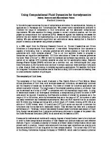
One of the simplest open channel controls is a rectangular drop structure, like the one shown in Figure 5. Rajaratnam and Chamani (1995) studied this type of drop structure, and organized a series of laboratory tests by altering the critical depth, Yc, to drop height, H, ratio over a range between 0.06 to 0.35. The primary downstream features of this two-dimensional drop are the height of the pool, Yp, and the pool length, Lp.
Figure 5 Schematic diagram of the drop structure test case [from Rajaratnam and Chamani (1995)].
Pacific Northwest National Laboratory
April 2001
10
For the purposes of this validation test, a single Yc/H ratio of 0.25 was selected. Since the reported results were also non-dimensional, a Yc of 0.5 m (H of 2.0 m) was selected. A uniform width of 0.5 m was used (all dimensions must be specified in FLOW-3D), and a constant inflow of 0.55 cms was specified at the upstream boundary of the test flume.
Figure 6 Numerical solution (FLOW-3D) of the Drop Structure test case. Velocity contours are in m/s and abscissa and ordinate units are in meters. Water depths in pool oscillate in time.
Based upon empirical data, Henderson (1966) states that the brink depth, Yb, should equal 0.715 Yc, and that critical depth should occur approximately 3 to 4 Yc upstream of the brink. With the assumed Yc for the test case, Yb should therefore equal 0.36 m, with a corresponding brink velocity, Vb, of 3.08 m/s. Time averaged values obtained from the laboratory flume and hydrodynamic model are as follows: At 2 m upstream of the brink Variable Measured Simulated Y/H 0.25 0.24 At the brink Variable Measured Simulated Yb/H 0.18 0.15 Vb 3.10 3.30
Downstream of the brink Variable Measured Simulated
φ
57
55
Y1/H
0.09
0.08
Yp/H
0.41
0.37
Lp/H
1.09
0.95
Figure 7 Comparison of results for the Drop Structure test case. Measured values are from Rajaratnam and Chamani (1995). Simulated values are from FLOW-3D. All values are dimensionless, except for Vb in m/s.
Pacific Northwest National Laboratory
April 2001
11
Model results generally matched observed values, with the worst error ratio occurring at the brink. At this location, the simulated depth was smaller by 0.03 m, resulting in an increase of simulated velocity by 0.2 m/s. The impact angle was also 2-degrees smaller than the observed angle of 57-degrees. The downstream plunge pool was observed to oscillate in time, and numerous undulations were noted in the water surface. The transient nature of the jet and plunge pool was also observed in the laboratory flume. Values reported in the paper were time-averaged, so some discrepancy between observed and simulated results should be expected.
3.3.
John Day Spillway
A single spillway bay at John Day Dam was simulated to test the ability of FLOW-3D to simulate large scale free-surface hydrodynamic processes. Since observed velocity field data along the spillway face and downstream tailrace were unavailable, this test was designed around a laboratory test documented in NHC (1999). CFD model geometry was constructed at prototype scale, however, and was not scaled to the laboratory flume. Model results were graphically compared to the physical model to qualitatively assess the abilities of the model to produce similar results. The following boundary conditions were specified for this test case: flow per bay = 5700 cfs, forebay elevation = 263.0 ft, tailrace elevation = 166 ft, spillway crest elevation = 210 ft, top elevation of spillway deflector = 153 ft, deflector submergence = 13 ft, gate opening = stop no. 4 [G0 = 2.90 ft, bottom elevation = 211.79 ft]. These boundary conditions, with the deflector in place, represents a duplication of test 5-11, NHC (1999).
Figure 8 Longitudinal slice through 3-D numerically modeled domain. Contours are of velocity magnitude (ft/s). Abscissa and ordinate axis dimensions are in feet. Vertical datum is mean sea level.
Pacific Northwest National Laboratory
April 2001
12
Figure 9 Physical model results [from NHC (1999)]. Figure caption is as follows: “Submergence 13.0 ft. A hydraulic jump is forming immediately downstream from the deflector”
Figure 10 FLOW-3D results along the spillway centerline – with deflector case. Contours are of velocity magnitude and legend is the same as in Figure 8. Water depths in the tailrace oscillate in time.
Figure 11 FLOW-3D results along the spillway centerline - no deflector case. Contours are of velocity magnitude and legend is the same as in Figure 8. Water depths in the tailrace oscillate in time.
Figures 9 and 10 compare the NHC (1999) scale model to the numerically simulated results. Simulated results have been contoured by velocity magnitude, and the large clockwise gyre downstream of the deflector has been emphasized with red arrows. As the water circulates in this gyre, a stagnation point occurs along the flume bottom between the deflector and the downstream energy dissipater. At this location flow either returns back towards the deflector or continues downstream.
Pacific Northwest National Laboratory
April 2001
13
Figures 10 and 11 compare simulated results with and without the deflector in place. Without the deflector, the clockwise gyre is no longer present downstream of the spillway, however a weaker counter-clockwise gyre circulates water throughout the tailrace pool. The water surface elevation of the tailrace pool ungulates in time for both cases, and the presented figures display only a single snapshot. The primary weakness of the numerical model is that air is not entrained by the falling water or in the turbulent tailrace zone. The plunging jet may sink deeper into the water column since the positively buoyant air is not accounted for, and water velocities may be higher at deeper depths. This shortcoming may be overcome by adding a calibrated point source of air along the upper portion of the spillway, although this option in FLOW-3D was not tested due to lack of observed data. Ideally, injected air would travel downstream with the water, and in the tailrace pool, the air would rise to the surface as buoyant forces overcame hydrodynamic advection. The rate of air injection would need to be calibrated however, and some observed hydrodynamic data in the tailrace pool would be required for calibration to be performed.
Pacific Northwest National Laboratory
April 2001
14
4 Application to the Bonneville Second Powerhouse Outfall and Tailrace Each application of a CFD model calls for its own unique set of challenges to be overcome. Several steps are common however to the Bonneville high flow outfall and tailrace modeling applications. First, structural and bathymetric data were obtained that completely described the fluid domain. This data was then manipulated into a format that could be imported into the 3-D hydrodynamic model FLOW-3D (STAR-CD was used only in the tailrace, see pg. 27). A 3-D computational boundary was created whose bottom surface conformed to the bathymetry and whose upper surface was set above the air-water interface. Initial and boundary conditions were assigned including inflow, downstream water surface elevation, and bottom roughness. The hydrodynamic model was executed until transient results reached a pseudo-steady-state condition, when results were then exported into visualization software and compared to observed data. Depending upon simulation results, model parameters were iteratively adjusted until variations between observed and simulated data were minimized. The most sensitive model parameters were found to be grid size and boundary roughness. The bounding hexahedron in FLOW-3D was split into numerous smaller hexahedrons by specifying a side length for the interior cells in each Cartesian direction (i.e. specifying the ∆x, ∆y, and ∆z for each interior cell). Typical side lengths ranged from less than 1.0 to more than 15 ft. Generally the volume of the interior cells were decreased in areas of large velocity gradients, and increased in zones where the flow field was more uniform. Boundary roughness in FLOW-3D is calculated by using wall functions to approximate the assumed logarithmic velocity distribution. Values used for the laboratory comparisons were typical for smooth surfaces, and were roughened for the prototype simulation. Note that all 1:30 scale physical model results were reported at prototype scale, however numerical simulations in this section were performed at prototype (1:1) scale.
4.1.
Skimming Outfall: Comparison to 1:30 scale model
The skimming high flow outfall case examined hydrodynamic conditions when the invert elevation of the sluice chute is located several feet below the water surface elevation of the tailrace. This test, also known as Test 4 (ENSR, 2000), places the invert at 0.25 ft msl (mean sea level) and the tailwater elevation at 8.5 ft msl. A flow of 5300 cfs exits the sluice chute at all times during the simulation. The bottom of the test flume is flat at elevation –22 ft msl.
Pacific Northwest National Laboratory
April 2001
15
Figure 12 Skimming test case: 3-D perspective of the velocity contours (ft/s).
In the 1:30 scale physical model, ambient cross flows, approximating flows emanating from the Second Powerhouse, were allowed to enter from the upstream and right (facing downstream) sides of the flume. These velocities were set in the 1:30 scale physical model by adjusting weirs and vanes on the headbox until velocities at 60% of the depth approximately matched those collected in the Waterways Experiment Station 1:100 scale physical model. Flow was allowed to exit the flume along the left and downstream ends of the flume, however ENSR (2000) found it difficult to match the 1:100 scale values along the left side (velocities were generally too low). The numerical model simulated ambient cross flows by using the average of reported velocities along each side of 1:30 scale physical model. Although the numerical model allows for spatially variable inflow boundary conditions, it seemed unreasonable to do this given the limited spatial resolution of the physical model dataset. In addition, because the water surface elevation was fixed in the numerical model, changes in velocity along the inflow boundary imply a change in flow rate. These velocity changes, which were reported at discrete locations in the physical model, induced surface waves in the numerical model, which then oscillated throughout the model domain and impacted the outfall jet. To remove these spurious waves, a uniform flow rate was applied along each side of the simulated domain by averaging the observed velocities along the same side. Figure 12 shows a 3-D perspective of the skimming case results using FLOW-3D. Contours of velocity reveal the impact of ambient cross flows as the jet slowly meanders back and forth. Turbulence was calculated using the RNG method, and results varied over time as eddies formed, separated from the jet mid-line, and were then washed out of the flume.
Pacific Northwest National Laboratory
April 2001
16
Figure 13 shows the location of the five data cross-sections reported in ENSR (2000). At the left edge of the figure, the sides of the outfall can be seen in black. The cross sections are located at the following distances downstream from terminus of the outfall: 30 ft, 60 ft, 90ft, 180 ft, and approximately 300 ft. Observed and simulated velocities were compared at these five locations. As Figures 14 and 15 show, the model captures the general trend of the jet outfall velocities, however differences do exist, primarily at cross-section 4. These differences have been quantified in Table 1 by computing mean velocity magnitudes and root mean square (RMS) errors, which have been calculated as: 1
n 2 2 O − S ( ) i ∑ i RMS = i =1 n
(1)
where O are observed magnitudes, S are simulated magnitudes, and n are the number of points along the cross-section. Differences changed over time as eddies broke off and were washed downstream. At the time-step snapshot shown in Figure 13, one can see that the mid-line of the jet has been pushed to the left (facing downstream) by the cross-stream flow. If the simulated jet were sampled at a time-step where the centerline had shifted slightly to the right, RMS errors between simulated and observed magnitudes would be less at cross-section 4. However, at cross-section 5, the match at the current time-step is quite close, with the simulated jet centerline more closely matching observed data, and a shift in jet location would cause the RMS error along this cross-section to rise. In summary, simulated results at cross-sections 1 through 3 matched to a reasonable error tolerance, with RMS errors less than 25% of the mean. Downstream of these crosssections, however, results differed over time. At the time step shown here, RMS errors were more than 50% of the mean at cross-section 4, however downstream at cross-section 5, RMS errors were less than 25%. This shows the time varying nature of the flow field, and hints at the expected velocity variations about the mean. Unfortunately no information was available regarding the range of observed time varying velocities, and only time-averaged means were presented in ENSR (2000).
Pacific Northwest National Laboratory
April 2001
17
Figure 13 Location of the five data cross sections sampled in the skimming case.
Table 1 Skimming Case: mean velocity and RMS error by cross-section
Section 1 2 3 4 5
Pacific Northwest National Laboratory
Mean Mag (ft/s) 23.09 21.03 17.32 14.51 11.38
RMS Err (ft/s) 5.48 1.43 3.16 7.36 2.49
RMS/Mean (%) 24% 7% 18% 51% 22%
April 2001
18
Figure 14 Skimming case: plan view velocity comparison. Red arrows are simulated (FLOW-3D) and blue arrows are physical model data.
Figure 15 Skimming case: side view velocity comparison. Red arrows are numerically generated (FLOW-3D) and blue arrows are physical model data.
Pacific Northwest National Laboratory
April 2001
19
4.2.
Cantilever Outfall: Comparison to 1:30 scale model
The general setup for the cantilever outfall case is identical to the skimming case except that the invert elevation of the sluice chute was raised to 26 ft msl. This test is also known as Test 5, ENSR (2000), and operated with an outfall discharge of 5300 cfs. In contrast to the skimming case, the outfall jet now exits from the chute above the tailrace pool, falls through the air, and impacts the water surface approximately 38 ft downstream from the chute’s terminus.
Figure 16 Skimming case: 3-D perspective of the velocity contours (ft/s).
One of the most significant aspects of numerically simulating the cantilever outfall is that of capturing the upper and lower water surface of the falling jet correctly. If the jet exit velocity is too fast or slow, the numerical solution will be different from that point onwards. As Figure 17 shows, FLOW-3D captured the upper and lower water surfaces of the falling jet with reasonable success. The camber of the simulated jet is slightly less than those observed in the 1:30 scale model (ENSR, 2000), causing the simulated jet to travel slightly farther. This could be due to a number of factors, the most significant of which may be the conditions in the sluice chute itself. The physical model contains an upstream headbox to regulate flow entering the chute, with a sharp crested weir to govern water height. Water velocities in the physical model channel were not reported and conditions in the numerical model were approximated by matching depth (and quantity) of flow at the terminus of the chute. No attempt was made to simulate the hydraulics in the 1:30 scale headbox.
Pacific Northwest National Laboratory
April 2001
20
Figure 17 Cantilever case: location of the free-falling jet. Dots are physical model data (observed) upper and lower water surfaces. Velocity contours are in ft/s.
Downstream of the jet impact location, velocities at five cross-sections were measured in the physical model (see Figure 18). Table 2 compares observed and simulated results across these cross-sections with RMS errors calculated using Equation 1. At cross-section 1, vertical components of the simulated water velocities were larger than observed. Water velocities at this location, no more than 10 ft (prototype scale) from where the jet enters the tailrace pool, vary dramatically depending upon the entry location of the falling jet. In the numerical model, the camber of the jet differed from the measurements, and the jet traveled farther towards cross-section 1. Since there was less distance between the impact location and cross-section 1 in the numerical model, this may explain the higher simulated velocities at this location. Differences between observed and simulated velocities downstream of cross-section 1 may result from the following: differences in air concentration of the falling jet between the two models, the transient nature of the test case, and the representative prototype scale size of the sampling volume observed by the velocity probe in the 1:30 scale physical model. At present, physical processes that describe the entrainment of air by the falling jet are beyond the capabilities of FLOW-3D. Although not attempted, it is possible in FLOW-3D to insert a point source of air into the falling jet, however the rate of injected air would need to be calibrated to field or published [e.g. Wood (1991)] data. Downstream of impact, a plunging jet with air (i.e. positively buoyant) will cause velocities throughout the entire water column (primarily along the jet centerline) to increase. In contrast, jets without air (i.e. neutrally buoyant) will primarily cause bottom velocities to increase, leaving the upper portion of the water column along the jet centerline only slightly energized. These differences are evident by the large RMS errors shown in Table 2, where the model overshot velocities along the bottom of the flume, and under predicted velocities above the jet centerline. It should be noted however that the neutrally buoyant case with zero entrained air is the more conservative case with regard to maximum depth and horizontal extent of the plunging jet. Pacific Northwest National Laboratory
April 2001
21
Figure 18 Location of the five data cross sections sampled in the cantilever case. Red arrows are numerically generated (FLOW-3D) and blue arrows are physical model data.
Figure 19 Cantilever case: plan view velocity comparison. Red arrows are numerically generated (FLOW-3D) and blue arrows are physical model data. Table 2 Cantilever Case: mean velocity and RMS error by cross-section
Section 1 2 3 4 5
Pacific Northwest National Laboratory
Mean Mag RMS Err RMS/Mean (ft/s) (ft/s) (%) 25.98 20.49 79% 21.38 13.66 64% 13.91 6.55 47% 10.25 6.32 62% 7.87 6.83 87%
April 2001
22
4.3.
Prototype: Development of bathymetric data
Bathymetric data surrounding the high flow outfall and tailrace were obtained from a 1998 survey (USACE, 1998). These points, plotted as discrete points in Figure 20, were the basis for the prototype CFD model grid.
direction of flow
Figure 20 Bonneville Second Powerhouse bathymetric survey data points. Note: density of the bathymetric dataset causes the discrete points to appear as lines in the figure.
Coverage downstream and to the north of the sluice chute outfall is quite detailed, however bathymetry values along the south side of the outfall were not gathered. Depths in this area were estimated based upon field observations made in October 2000. Figure 21 and Figure 22 present a 3-D perspective of these bathymetric points. The deepest portions of the tailrace are located immediately downstream of the Powerhouse and reach elevations of less than –60 ft msl. Bottom elevations slope dramatically upwards from the Powerhouse and quickly reach an average thalweg elevation of approximately –20 ft msl.
Pacific Northwest National Laboratory
April 2001
23
Figure 21 Tailrace bathymetry at the Bonneville Dam Second Powerhouse. Inset shows the filled channel.
Figure 22 Tailrace bathymetry near the high flow outfall exit. Inset shows the channel filled with water to elevation 11 ft. Datum is mean sea level.
Pacific Northwest National Laboratory
April 2001
24
4.4.
Prototype Outfall and Tailrace: October 3, 2000
Between 9 and 11 a.m. on October 3, the high flow outfall was operated at a flow of 2500 cfs, the tailrace elevation was approximately steady at 11.0 ft msl, and turbine units 11, 12, and 14 through 18 were operating. FLOW-3D was used to simulate these conditions, and results are summarized graphically in the following figures. Figure 23 displays a 3-D perspective of the outfall. Near the outfall, surface velocity vectors have been placed on top of velocity magnitude contours. The color contour scale has been set to show velocity variation in the tailrace pool, causing the jet to be displayed as red, indicating magnitudes above 10 ft/s.
Figure 23 3-D perspective of the Oct 3, 2000 prototype case simulation
Figure 24 shows a downstream oriented perspective of the outfall and tailrace pool, and a cutting plane of velocity magnitude has been placed along the centerline of the outfall. The velocity magnitude of the simulated jet at the outlet terminus was approximately 40 ft/s. When the jet impacted the tailwater, its magnitude had increased to approximately 54 ft/s, which corresponds with theory (54.3 ft/s). Magnitudes decreased rapidly as the jet plunged into the tailrace. After impact, the jet was quickly diverted upwards and to the left (south) side of the river by the scour hole and ambient cross-flow conditions. At the downstream edge of the scour hole, magnitudes increased again as the flow converged over the top of the scour hole, as shown by the red zone downstream of the jet in Figure 23 and Figure 25.
Pacific Northwest National Laboratory
April 2001
25
Figure 25 displays a plan view perspective of the high flow outfall. Simulation results indicate the formation of a counter clockwise gyre that formed to the left (south) of the jet entry point. This gyre extended downstream until approximately the end of the scour hole. These simulated results correspond well to observations made using a GPS tracked drogue during this test case (see Cook, et al. [2001] for additional details). Figure 26 shows the flow path of the surface drogue released north and upstream of the outfall. The drogue was entrained in the surface gyre for several seconds, before it exited and traveled downstream.
Figure 24 Velocity ribbon through the jet centerline for the Oct 3, 2000 prototype test case
Pacific Northwest National Laboratory
April 2001
26
Figure 25 Plan view perspective for the Oct 3, 2000 prototype test case. All velocities at or above 10 ft/s are shown in red.
Figure 26 Path of drogue released upstream of the outfall at 2500cfs [from Cook, et al. (2001)]. The drogue was released from the right side of the outfall (red square), and was entrained by the counter-clockwise gyre. After circulating twice around the gyre, the drogue then exited and traveled downstream.
Pacific Northwest National Laboratory
April 2001
27
4.5.
Prototype Tailrace: February 7, 2000. Comparison to ADCP
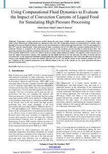
Figure 27 through Figure 29 compare 3-D hydrodynamic model results to measured velocities collected downstream of the Second Powerhouse. Acoustic Doppler current profiler (ADCP) velocity data were measured between 8:00 and 12:00 on February 7, 2000, when all units of the powerhouse were operating (ENSR, 2000b). Average discharge from the powerhouse during this period was approximately 141,100 cfs. Once the 3-D computational meshes were developed, appropriate boundary conditions for the period were developed for both FLOW-3D and STAR-CD. STAR-CD was operated in steady-state mode, which may be appropriate for the time invariant discharges through the Powerhouse turbines. FLOW-3D was operated in a transient mode, although a constant discharge exited through the powerhouse at all times, and the model was operated until quasisteady conditions were reached. Simulated velocity magnitude contours, plus vectors at ADCP locations, are shown for three different elevations (Figures 26-28) and Table 3 shows the mean magnitude and RMS errors by depth. RMS errors are slightly higher for FLOW-3D, however the RMS errors for both models are approximately equal to the mean ADCP standard deviation of 0.9 ft/s. Figure 30 displays observed versus simulated results for all velocity magnitudes shown in Figures 26-28 (i.e., all three depths). The standard deviation has been placed for each measurement. A perfect correlation between model and prototype would exist if all symbols in the figure fell along the diagonal 45-degree line. Out of the 90 observed values, 82% (74 locations) of the STAR-CD and 46% (41 locations) of the FLOW-3D values fell within 1-standard deviation of the observed ADCP values. Likewise 99% (89 locations) STAR-CD and 99% (89 locations) FLOW-3D values fell within 2-standard deviations of the observed. Note that FLOW-3D was not calibrated for this application, unlike STAR-CD, which was calibrated by adjusting bottom roughness. Although FLOW-3D results appear slightly worse than STAR-CD, both models simulate the general flow regime within the observed velocity fluctuations. Table 3 Mean Magnitudes and RMS Errors by Depth for Both Models. Note: The mean ADCP standard deviation was 0.9 ft/s (approx. 18% of the mean)
STAR-CD Elevation Mean Mag RMS Err RMS/Mean (ft) (ft/s) (ft/s) (%) +3' 5.01 0.70 14% -6' 4.92 0.64 13% -14' 4.84 0.49 10%
Pacific Northwest National Laboratory
FLOW-3D RMS Err RMS/Mean (ft/s) (%) 1.08 22% 0.94 19% 0.84 17%
April 2001
28
Figure 27 Numerical simulation results versus observed data at +3 ft elevation. Red arrows are ADCP observations (ENSR, 2000b), blue arrows are from STAR-CD, and black arrows are from FLOW-3D.
Figure 28 Numerical simulation results versus observed data at -6 ft elevation. Red arrows are ADCP observations (ENSR, 2000b), blue arrows are from STAR-CD, and black arrows are from FLOW-3D.
Pacific Northwest National Laboratory
April 2001
29
Figure 29 Numerical simulation results versus observed data at -14 ft elevation. Red arrows are ADCP observations (ENSR, 2000b), blue arrows are from STAR-CD, and black arrows are from FLOW-3D.
simulated FLOW-3D or STAR-CD (ft/s)
8 7 6 5 4 3 2
STAR-CD FLOW-3D
1 0 0
1
2
3
4
5
6
7
8
observed ADCP (ft/s)
Figure 30 Observed [ADCP data from ENSR (2000b)] versus simulated results for the three elevations (+3, -6, and –14 ft). Horizontal bars represent reported standard deviations of the ADCP measurements.
Pacific Northwest National Laboratory
April 2001
30
5 Full Tailrace Model The extent of the STAR-CD model was enlarged to cover the entire tailrace below the Bonneville Project as a “proof-of-concept”. The model was run in steady-state mode, using boundary conditions that approximated tailrace conditions on February 7, 2000. The simulation results shown here were generated before the model was calibrated (in contrast to Section 4.5), and are with a lower Manning roughness. The impact of lowering the roughness is most evident along the shoreline near where the Section 4.5 model ends. Note that during this period, all of the units of the 2nd Powerhouse and approximately half of the 1st Powerhouse were operating (Units 4-8 and 10 reported less than 2 kcfs passing through the turbines). No flow was released from the spillway during this period.
Figure 31 STAR-CD simulation results for the entire Bonneville Project Tailrace.
Pacific Northwest National Laboratory
April 2001
31
6 Conclusions The primary objective of this project was to investigate the feasibility (i.e. “proof-ofconcept”) of using computational fluid dynamics (CFD) models to simulate tailrace, high flow outfall, and general free-surface non-hydrostatic problems typically encountered near hydraulic structures. The initial task was to survey relevant technical literature and to evaluate various CFD models capable of simulating free-surface breakup and the physics of plunging jets. Two numerical models were selected for further analysis: STAR-CD and FLOW-3D. The methodology used by STAR-CD to simulate the free-surface was found to be inadequate since in frothy, turbulent zones (like those typically found under a free-falling jet) a sharp interface is difficult to maintain with a reasonably large grid size. It was for this reason that FLOW-3D was selected and verified for use to simulate high flow outfalls. Three validation cases were selected to test FLOW-3D. The first case simulated a generic hydraulic jump in a long rectangular flume. Results compared well against observed water depths both before and after the jump. The second test case simulated a rectangular drop structure. Results were compared with published data, and the simulated values again matched observed within a reasonable error tolerance. The third case simulated a single spillway bay at John Day Dam. Although only a qualitative comparison of water depths downstream of the radial gates is possible, the overall water profile generally followed those reported in NHC (1999). FLOW-3D results are presented for two structural configurations of the spillway bay: with and without a downstream deflector. This comparative test was performed to demonstrate the use of CFD models as management tools for evaluating hypothetical modifications to hydraulic structures. Once the model was validated against these three test cases, it was applied to the Bonneville Second Powerhouse. Two general bathymetries were configured as input to the model: a) at prototype scale, but conforming to the 1:30 scale physical model simplifications, and b) prototype scale, representing actual bathymetric conditions. The physical model constructed by ENSR (2000) allowed for direct comparison of velocity fields between physical and numerical models. Comparisons were performed when the outfall invert was just below the water surface (skimming case) and 17.5 ft above the tailrace water surface (cantilever case). FLOW-3D successfully captured the general velocity field for both of these test cases, although differences between observed and simulated were less in the skimming case. Differences in the cantilever case may be due to the lack of air being entrained by the falling jet in FLOW-3D. Differences may also be due to a difference in scale since the physical model was at 1:30 and the numerical was at prototype. Both STAR-CD and FLOW-3D were then applied to the tailrace area downstream of the Second Powerhouse. Model results were compared at three different depths to observed water velocities gathered on February 7, 2000. Differences between observed and simulated velocities were within 1- to 2-standard deviations of observed magnitude variations, indicating that both models are appropriate for simulating zones where the free surface is continuous (i.e. unbroken).
Pacific Northwest National Laboratory
April 2001
32
7 Future Applications FLOW-3D should be considered suitable for application to free-surface non-hydrostatic flow. At this time applications best suited for this model are ones of small geographic extent, primarily due to the relatively small grid size, and hence long simulation times, necessary to capture free-surface breakup. Several issues regarding the simulation of a free-surface jet remain unanswered, although a “conservative” model without air entrainment is documented in this report. These issues involve: (1) the entrainment of air by the falling jet, (2) the simulation of bubbles within the flow field, and (3) spatial scale differences between physical and numerical models. Several options exist to handle the first two issues. In the most recent version of FLOW3D, it is possible to simulate bubbles that have been introduced into the flow field, although due to time constraints this option was not tested. Pressure inside of a simulated submerged bubble, which will vary depending upon its depth beneath the water surface, could be tracked with a corresponding change in bubble volume. Simulated bubbles may also break up or coalesce as they move through the domain. Further testing of these option may improve results for the cantilever outfall, drop structure, and spillway cases, however entrainment of air would still need to be approximated by a calibrated source placed in the falling jet. If suitable data were available (such as observed percent air concentrations measured in the falling jet and downstream plume), spherical bubbles of various diameters could be placed in the jet and simulated from that location onwards. Published laboratory test cases and design guides, such as Wood (1991), may also provide further guidance and suitable verification and calibration test cases for this rapidly advancing area of CFD. For the third issue, it is proposed that future comparisons/verifications of the numerical model be performed at the same scale as the observed data for cases with significant air entrainment. In Sections 3.3, 4.1 and 4.2 of this report, the scale of the numerical model was prototype while the scale of the observed data (physical model) was much less than prototype. In contrast, Sections 3.1, 3.2, and 4.5 compare observed data and numerical model results where both datasets are at the same scale (either laboratory/laboratory or prototype/prototype). Since both the prototype and numerical model can be unsteady, data at equal scales allows for comparison of transient phenomenon, such as velocity variations about the mean. Therefore it is recommended that the physical dimensions and time scales should be equal between numerical model and observed data to ensure a complete match of Froude, Reynolds, and Webber numbers for cases with significant air entrainment. FLOW-3D is capable of simulating variable density particles that have been placed by the user into the flow field. Particles can be assigned a mass and density (if not, they are neutrally buoyant) so as to interact with the flow field. Drag forces on the particles are calculated, and can be scaled to the Reynolds number. These particles can be used to simulate any number of scalars in the flow field, including fish (as long as their behavior can be described as Gaussian), dye, and air bubbles. For example if Rhodamine dye were simulated, properties of the dye would be used as input to describe the particles (viscosity, density, quantity to be injected, etc.). Time evolution of dye concentrations could then be simulated to help visualize
Pacific Northwest National Laboratory
April 2001
33
the flow field. Simulated dye paths could also be used to determine the sensitivity of both the numerical (due to turbulence approximations, numerical schemes, grid size, etc.) and the physical (Froude number similitude approximations, bathymetric simplifications, etc.) models to fluctuations in operating conditions. Finally, FLOW-3D and STAR-CD have the ability to simulate moving obstacles. A rotating obstacle could be used to simulate turbines, fan blades, wicket gates, and radial gates. Translating obstacles could be used to represent navigation locks and vertically moving gates, which are ubiquitous as hydraulic controls. Combined with appropriate behavior models for fish, these CFD tools are capable of isolating the optimum design from a suite of options, usually in a rapid manner, and with quantitative statistics on differences between designs.
Pacific Northwest National Laboratory
April 2001
34
References Adapco, (2000). Adapco web page URL: http://www.adapco.com CD, (2000). Methodology Guide, STAR-CD version 3.10, Computational Fluid Dynamics Limited. CD, (2000b). Computational Dynamics web page URL: http://www.cd.co.uk C.B. Cook, M.C. Richmond, G. R. Guensch (2001) Bonneville Second Powerhouse Tailrace and High Flow Outfall: ADCP and drogue release field study, PNNL-13403, Pacific Northwest National Laboratory, 25 pgs. ENSR (2000). Bonneville Second Powerhouse Corner Collector Outfall: 1:30 Scale Physical Hydraulic Model, 60% Submittal, ENSR Corporation, Document Number 3697-002-400, June. ENSR (2000b). Bonneville Second Powerhouse Tailrace ADCP Field Data Collection Report: Final Report, ENSR Corporation, Document Number 3697-003-106A, March. FI, (2000). Fluent Inc. web page URL: http://fluent.com FI, (2000b). Fluent Inc. applications URL: http://fluent.com/solutions/index.htm Freitas, C.J. (1995). “Perspective: Selected Benchmarks from Commercial CFD Codes,” Transactions of the ASME, 117, pp 208-218. FSI, (2000). Flow Science Inc. web page URL: http://test.FLOW-3D.com Gharangik, A.M. and M.H. Chaudhry (1991). “Numerical Simulation of Hydraulic Jump”, Journal of Hydraulic Engineering, American Society of Civil Engineers, 117(9), September. Hirt, C.W. and Nichols, B.D. (1981). "Volume of Fluid (VOF) Method for the Dynamics of Free Boundaries," Journal of Computational Physics, 39(201). Henderson, F.M. (1966). “Open Channel Flow”, MacMillian Publishing Co., New York. Kothe, D.B, R.C. Mjosness, M.D. Torrey (1991). “RIPPLE: A Computer Program for Incompressible Flows with Free Surfaces,” Los Alamos National Laboratory Report LA12007-MS. Nichols, B.D., C.W. Hirt, R.S. Hotchkiss (1980). “SOLA-VOF: A Solution Algorithm for Transient Fluid Flow with Multiple Free Boundaries,” Los Alamos Scientific Laboratory Report LA-8355. NHC (1999). “John Day Dam Sluice Model, Hydraulic Model Study Final Report,” Northwest Hydraulic Consultants (NHC), report prepared for US Army Corps of Engineers – Portland District, January 1999. Perkins, W.A. and M.C. Richmond (1999) Long-Term, One-Dimensional Simulation of Lower Snake River Temperatures for Current and Unimpounded Conditions, Report submitted to U.S. Army Corps of Engineers, Walla Walla District, Pacific Northwest National Laboratory, Richland, WA. Pacific Northwest National Laboratory
April 2001
35
Rajaratnam, N. and M.R. Chamani (1995). “Energy loss at drops”, Journal of Hydraulic Research, 33(3), pp 373-384. Rakowski, C.L., and M.C. Richmond (2000). Dalles Tailwater Predator Study: Numerical Analysis of Tailwater Flow Conditions. Report submitted to U.S. Army Corps of Engineers, Portland District, Pacific Northwest National Laboratory, Richland, WA. Rakowski, C.L., M.C. Richmond, G.R. Guensch, and J.A. Serkowski (2000). Bonneville Project Adult Migrant Fallback Study Application of 2D and 3D Flow Simulations to Upstream Migration and Operational and Structural Alternatives, Report submitted to U.S. Army Corps of Engineers, Portland District, Pacific Northwest National Laboratory, Richland, WA. Richmond, M.C., W.A. Perkins, and Y. Chien (2000) Numerical Model Analysis of SystemWide Dissolved Gas Abatement Alternatives. Report submitted to U.S. Army Corps of Engineers, Walla Walla District, Battelle, Pacific Northwest Division, Richland, WA. Torrey, M.D., R.C. Mjolsness, L.R. Stein (1987). “NASA-VOF3D: A Three-Dimensional Computer Program for Incompressible Flows with Free Surfaces,” Los Alamos National Laboratory Report LA11009-MS. USBR, (2000). US Bureau of Reclamation, Water Resources Research Laboratory web page USR: http://www.usbr.gov/wrrl/wc/wm/numerical.html USACE (1998). Data provided by Portland District, US Army Corps of Engineers. Wood, I. R. (1991). Air Entrainment in Free-Surface Flows, Hydraulic Structures Design Manual No. 4, IAHR, Balkema.
Pacific Northwest National Laboratory
April 2001