Aug 13, 1996 - (b) mesh1 mesh2 mesh3 mesh4 mesh5. -5. 0. 5. 10. 15. 20. 25. 30. 35. -3. -2.5 .... Further financial support by AKZO-Nobel, Philips Electronics,.
Simulation of viscoelastic flows using Brownian configuration fields∗ M.A. Hulsen A.P.G. van Heel B.H.A.A. van den Brule Delft University of Technology, Laboratory for Aero and Hydrodynamics, Rotterdamseweg 145, 2628 AL Delft, The Netherlands August 13, 1996
Abstract In this paper we present a new approach for calculating viscoelastic flows. The polymer stress is not determined from a closed-form constitutive equation, but from a microscopic model. In this description, we replace the collection of individual polymer molecules by an ensemble of configuration fields, representing the internal degrees of freedom of the polymers. Similar to the motion of real molecules, these configuration fields are convected and deformed by the flow and are subjected to Brownian motion. We incorporated this field description in a finite element calculation. An important advantage of our approach is that the difficulties associated with particle tracking of individual molecules are circumvented. In order to validate our approach and to demonstrate its robustness, we present the results for the start-up of planar flow of an Oldroyd-B fluid past a cylinder between two parallel plates. The results are very promising. We find excellent agreement between the results of the configuration field formulation and those obtained using a closed-form constitutive equation. Moreover, the microscopic method appears to be more robust than the conventional macroscopic technique. keywords: Finite element method, Brownian Dynamics, Configuration fields.
1
Introduction
The field of viscoelastic fluid research has recently shown some exciting developments, which offer opportunities to study systems that are well beyond the limitations inherent to the conventional macroscopic approach. These limitations were due essentially to the need of a closed-form constitutive equation (CE) to complement the conservation laws of mass and momentum. This CE can either be founded on a macroscopic approach, i.e. within the framework of continuum mechanics, or on a microscopic description using kinetic theory. A comprehensive review of both approaches can be found in [1, 2]. Since the parameters in the CE depend on the material under investigation, they have to be determined from the measured material response in a well-defined deformation like shear and elongational flow. Once all parameters in a given CE have thus been determined, it can be used in a complex flow calculation. However, often discrepancies between numerical predictions and ∗ This
paper has appeared as: J. non-Newtonian Fluid Mech., 70 (1997) 79-101.
1
experimental results are found. A possible cause for these differences might be that the flow field in a rheometer is too simple to assess the validity of a CE. A way to overcome this problem is to carefully measure stress and velocity fields in a more complex situation, like flow past a cylinder, and to compare these measurements with numerical calculations. Depending on the results it might turn out that it is necessary to adjust the parameters or even to reject or improve the CE. Improvements, however, are constrained by the fact that in macroscopic calculations only closed-form CE’s can be used. This immediately rules out many of the microscopic models, often in spite of their intuitively more appealing description. Recently, a promising technique has been introduced to avoid the problems described above, by simply bypassing the need for a CE. The essential idea of this socalled CONNFFESSIT approach is to combine traditional finite element techniques and Brownian Dynamics simulations. An overview of the various approaches is illustrated in Fig. 1. In contrast to a conventional finite element approach, however, CONTINUUM
KINETIC
MECHANICS
THEORY
CONSTITUTIVE EQUATIONS
RHEOMETRY
BROWNIAN DYNAMICS
FLOW CALCULATIONS
Figure 1: Interrelation between various fields in fluid research. The left-hand side shows the conventional approach using continuum mechanics or kinetic theory and rheometry to obtain constitutive equations which can be used in macroscopic flow calculations. The alternative approach, avoiding the use of a CE, using Brownian Dynamics simulations of microscopic models derived within kinetic theory, is indicated on the right. the polymer contribution to the stress, needed in the finite element calculation, is not calculated from a CE, but instead from the configuration of a large ensemble of model polymers [3, 4, 5, 6]. The time evolution of this ensemble is calculated using Brownian Dynamics. Thus, for each model polymer the centre-of-mass trajectory is calculated from the velocity field, while the evolution of the molecule’s configuration is found by integrating the stochastic differential equations corresponding to the internal degrees of freedom of the model under consideration. This procedure can excellently be combined with macroscopic finite element calculations: the stress field is now calculated on the basis of the configurations of the polymers in each element. This approach has been shown to be able to reproduce the known analytical results for start-up flow of a Maxwell fluid for 1-D plane Couette flow [3] and start-up of 2-D flow between two concentric cylinders [7]. For problems for which no analytic solution is at hand, the method has been tested by comparing its results with those obtained using a purely macroscopic finite element calculation. The latter approach
2
was applied to the problem of steady flow of an Oldroyd-B fluid in an abrupt 4:1 axisymmetric contraction [8]. In this case the stress was either calculated from an ensemble of Hookean dumbbells or from the equivalent macroscopic Oldroyd-B equation. The most promising feature of the new approach, however, is its ability to calculate fluid flows using models for which no closed-form CE is known, such as e.g. a FENE model [3, 7, 9]. Additional advantages are that it is very easy to change models and that in principle it is possible to incorporate effects like chemical reactions, polydispersity, polymer migration etc.. In this paper we present a new approach to solve time dependent visco-elastic flows, based on an ensemble of Brownian configuration fields. The basic idea of this description is to replace the collection of individual molecules by an ensemble of configuration fields, representing the internal degrees of freedom (configuration) of the polymer molecules. An important feature of the configuration fields, as will be explained in section 2, is that in this approach the configurations are defined in every point of the domain. In analogy with the centre-of-mass convection and the evolution of the configuration of a real polymer molecule the fields are convected by the flow and are subjected to Brownian motion. Moreover, by the way we implemented the Brownian motion, the configuration fields are continuous. As we shall see in section 3, these properties make the method particularly suitable for implementation in a finite element formulation of the problem. A major advantage of the field description is the ease of incorporating convection into the simulation, thus avoiding the difficulties associated with the tracking of individual particles. In order to validate the configuration field method and to demonstrate its robustness, we consider in section 4 the start-up of planar flow of an Oldroyd-B fluid past a cylinder between two parallel plates. We solved this problem by two different methods: first by an entirely macroscopic calculation and then by using the configuration field formulation. In the first case the polymer contribution to the stress is calculated from the CE for an Oldroyd-B fluid, in the second case this stress is obtained from an ensemble of Hookean dumbbell configuration fields. A summary with conclusions is given in section 5. 2
Governing equations
The isothermal flow of an incompressible fluid with density ρ is governed by the momentum balance and the continuity equation: ρ
∂u + ρu · ∇u = −∇p + ∇ · τ , ∂t
(1)
∇ · u = 0.
(2)
In these equations p and u denote the pressure and the velocity field and τ is the extra stress generated in the fluid due to its motion. It is standard practice to write the extra stress of a polymer solution as the sum of a solvent contribution, τ s , and a contribution due to the presence of the polymer, τ p . For the solvent contribution we take the constitutive equation of a Newtonian fluid, i.e. τ s = 2ηs d where d = (∇u + (∇u)T )/2 is the rate-of-deformation tensor and ηs is the solvent viscosity. The momentum balance can thus be written as ρ
∂u + ρu · ∇u = −∇p + ∇ · (2ηs d + τ p ). ∂t
(3)
The polymer contribution to the stress can be calculated using a constitutive equation or from a Brownian Dynamics simulation. In this paper we will use the so-called Oldroyd-B model. This model finds its origin in continuum mechanics but it can 3
also be derived from a microscopic model. The Oldroyd-B constitutive equation reads 5 (4) τ p + λτ p = 2ηp d. In this equation λ is the relaxation time of the fluid, ηp is the polymer contribution 5 to the viscosity and τ p is the upper convected derivative of the stress, defined by 5 τ p = ∂τ p /∂t + u · ∇τ p − κ · τ p − τ p · κT , where κ is the transpose of the velocity gradient, κ = (∇u)T . From a microscopic point of view the Oldroyd-B equation is the result of the Hookean dumbbell model. In this model a polymer solution is considered as a suspension of non-interacting elastic dumbbells consisting of two Brownian beads with friction coefficient ζ connected by a linear spring. The configuration of a dumbbell, i.e. the length and orientation of the spring connecting the two beads, is indicated by a vector Q. The spring force can thus be written as F (c) = HQ where H is the spring constant. It can be shown that the probability ψ(Q, x, t)d3 Q of finding a dumbbell with a configuration Q at (x, t) is governed by the following equation �� � � ∂ ∂ 2HQ ∂ 2kT ∂ ∂ ψ=− · (uψ) − · κ·Q− · ψ. (5) ψ + ∂t ∂x ∂Q ζ ζ ∂Q ∂Q In Eq. (5) one recognises the various effects that alter the configuration distribution: convection, rotation and stretching of dumbbells due to the flow field, elastic retraction that wants to minimise the dumbbell length and the effect of thermal motion, or dumbbell diffusion. In case the configuration distribution is independent of spatial position the first term on the RHS vanishes and the equation reduces to the usual Fokker-Planck or diffusion equation [2]. Once the configuration distribution function ψ is known, it is possible to calculate the stress using the Kramers expression which for the dumbbell model reads τ p = −nkT 1 + nHhQQi,
(6)
where n is the number density of dumbbells and the angular brackets denote a configuration ensemble average Z (7) hf i = ψf d3 Q. So, in principle, following this scheme, one first has to solve the Fokker-Planck equation Eq. (5) to obtain the distribution function. Then, using the Kramers expression, the stress can be calculated. In practice this approach is very uneconomic, especially for models with more degrees of freedom, since it requires a numerical integration over a high-dimensional volume. Fortunately, for some models a direct closure is possible. For instance for the Hookean dumbbell model one can multiply the Fokker-Planck equation by QQ and integrate over all Q. Elimination of hQQi from the resulting equation with the use of the Kramers expression for the stress tensor finally yields the Oldroyd-B equation. It turns out that the relaxation time λ = ζ/4H and the polymer contribution to the viscosity is given by ηp = nkT λ. An alternative, but equivalent, approach for generating the configuration distribution is to make use of a stochastic differential equation. This means that the dynamics described by the Fokker-Planck equation can be considered as the result of a stochastic process acting on the individual dumbbells. For the details on the formal relationship between the Fokker-Planck equation and stochastic differential equations the reader is referred to [6]. For the Hookean dumbbell model considered here, the stochastic equation reads s � � 4kT 2H Q(t) dt + dW (t), (8) dQ(t) = κ(t) · Q(t) − ζ ζ 4
where W (t) is a Wiener process which accounts for the random displacements of the beads due to thermal motion. The Wiener process is a Gaussian process with zero mean and covariance hW (t)W (t0 )i = min(t, t0 )1. In a Brownian Dynamics simulation this equation is integrated for a large number of dumbbells. A typical algorithm, based upon an explicit Euler integration, reads s � � 4kT 2H Q(t) ∆t + ∆W (t), (9) Q(t + ∆t) = Q(t) + κ(t) · Q(t) − ζ ζ where the components of the random vector ∆W (t) are independent Gaussian variables with zero mean and variance ∆t. Once the configurations are known the stress can be estimated by τ p ≈ −nkT 1 + nH
Nd 1 X QQ, Nd i=1 i i
(10)
where Nd is the number of dumbbells and Qi represents the i th dumbbell in the ensemble. In order to solve a flow problem it is necessary to find an expression for the stress at a specified position x at time t. From a microscopic point of view this means that we have to convect a sufficiently large number of molecules through the flow domain until they arrive at x at time t. Neglecting centre-of-mass diffusion, these molecules all experienced the same deformation history but were subjected to different, and independent stochastic processes. However simple in theory, a number of problems have to be addressed in practice. For instance, if we disperse a large number of dumbbells into the flow domain we not only have to calculate all their individual trajectories but, to calculate the local value of the stress, we must every time step also sort all the dumbbells into cells (or elements). Another problem arises due to the fact that the tracking occurs with a finite accuracy so that we have to check for dumbbells leaving the flow domain through the boundaries. Once these problems are solved it is possible to construct a transient code to simulate a non-trivial flow problem. This has in fact been done by Laso et al. [7] for the start-up of flow in a journal bearing. We used a different approach to this problem which overcomes the problems associated with particle tracking. Instead of convecting discrete particles specified by their configuration vector Qi an ensemble of Nf continuous configuration fields Qi (x, t) is introduced. Initially, the configuration fields are spatially uniform and their values are independently sampled from the equilibrium distribution function of the Hookean dumbbell model. After start-up of the flow field the configuration fields are convected by the flow and are deformed by the action of the velocity gradient, by elastic retraction and by Brownian motion in exactly the same way as a discrete dumbbell. The evolution of a configuration field is thus governed by � � 2H Q(x, t) dt dQ(x, t) = −u(x, t) · ∇Q(x, t) + κ(x, t) · Q(x, t) − ζ s 4kT dW (t). (11) + ζ The first term on the RHS of Eq. (11) accounts for the convection of the configuration field by the flow. It should be noted that dW (t) only depends on time and hence it affects the configuration fields in a spatially uniform way. For this reason the gradients of the configuration fields are well defined and smooth functions of the spatial coordinates. Of course, the stochastic processes acting on different fields are uncorrelated. 5
From the point of view of the stress calculation this procedure is completely equivalent to the tracking of individual dumbbells: An ensemble of configuration vectors {Qi } with i = 1, Nf is generated at (x, t) which all went through the same kinematical history but experienced different stochastic processes. This is precisely what is required in order to determine the local value of the stress. In the remainder of this paper we prefer to scale the length of the configuration p vector with kT /H, which is one-third of the equilibrium length of a dumbbell. The relevant equations thus become: τ p = nkT (−1 + b) =
ηp (−1 + b), λ
(12)
˜ Qi ˜ is the conformation tensor, which is dimensionless and reduces to where b = hQ the unity tensor at equilibrium. The Oldroyd-B equation can now be written as 5
b + λb = 1. The equation for the evolution of the configuration fields becomes � � 1 ˜ ˜ ˜ ˜ Q(x, t) dt dQ(x, t) = −u(x, t) · ∇Q(x, t) + κ(x, t) · Q(x, t) − 2λ r 1 dW (t). + λ
(13)
(14)
Finally, the conformation tensor field follows from b(x, t) =
Nf 1 X ˜ ˜ (x, t). Q (x, t)Q i Nf i=1 i
(15)
From now on the tildes are dropped and it is understood that Q is a dimensionless quantity. 3 3.1
Numerical methods Preliminaries
For the spatial discretisation of the system of equations we will use the finite element method. In order obtain a better stability and extend the possible stress space, we use the Discrete Elastic-Viscous Split Stress (DEVSS) formulation of Gu´enette & Fortin [10] for the discretisation of the linear momentum balance and the continuity equation. The discontinuous Galerkin (DG) formulation will be used to discretise the constitutive equation in the macroscopic case and the equation for the configuration fields in the microscopic case. In the DG formulation the interpolation functions are discontinuous across elements, leading to a minimal coupling between elements. This means that in our time-stepping scheme the stresses and the configuration variables at the next time step can be computed at element level. In this way we avoid solving a large number of coupled equations, which in particular for the configuration fields would be an almost impossible task. The combination of the DEVSS formulation with DG has been introduced by Baaijens et al. [11] and leads to a remarkably stable method. 3.2
Momentum balance and continuity equation
We use the DEVSS formulation [10] for which we introduce an extra variable e = 2ηp d: the viscous polymer stress. We rewrite the momentum balance Eq. (1) 6
and the continuity equation Eq. (2) as follows ρ
∂u + ρu · ∇u + ∇p − ∇ · (2ηs d(u) + τ p ) − ∇ · (2ηp d(u) − e) = 0, ∂t
(16)
− ∇ · u = 0,
(17)
1 e = 0, − d(u) + 2ηp
(18)
where 2d(u) = ∇u + (∇u)T . Note that if we substitute Eq. (18) into Eq. (16) the last term on the LHS of Eq. (16) vanishes and we obtain Eq. (1) again. However in the discretisation step 2ηp d will differ from e and extra stability is obtained compared to the standard Galerkin formulation without e. For the weak formulation of Eqs. (16)–(18) we introduce separate functional spaces for u, p and e, which we denote by U , P and E, respectively. The weak formulation can be found by multiplying with testfunctions and integration by parts: find (u, p, e) ∈ U × P × E such that for all (v, q, f ) ∈ U × P × E we have (v, ρ
∂u + ρu · ∇u) − (∇ · v, p) + (∇v, 2ηd(u) − e + τ p ) = (v, σ)Γ , ∂t
(19)
− (q, ∇ · u) = 0,
(20)
− (f , ∇u) +
1 (f , e) = 0, 2ηp
(21)
where (·, ·) and (·, ·)Γ are proper L2 inner products on the domain Ω and on the boundary Γ, respectively. The viscosity η is the zero-shear-rate viscosity ηs + ηp and σ is the traction vector on the boundary. The system for (u, p, e) is symmetrical except for the ρu · ∇u term. The discrete form of the equations is obtained by requiring that the weak form is valid on approximating subspaces Uh × Ph × Eh which consist of piecewise polynomial spaces. The discrete solutions and the discrete testfunctions are denoted with subindex h : (uh , ph , eh ) and (v h , qh , f h ). In this work we use quadrilateral elements with continuous biquadratic polynomials (Q2 ) for the velocity space Uh , discontinuous linear polynomials (P1 ) for the pressure space Ph and continuous bilinear polynomials (Q1 ) for viscous polymer stress space Eh . 3.3
Constitutive equation
For the discretisation of the constitutive equation we use the discontinuous Galerkin method [12] which is best formulated on a single element. The first step is to multiply Eq. (13) with a testfunction s and integrate over a single element ei : � � 1 ∂b + u · ∇b − κ · b − b · κT + (b − 1) = 0, (22) s, ∂t λ ei where (·, ·)ei denotes an L2 inner product on element ei only. The second step is to integrate the convection term by parts: (s, u · ∇b)ei = (s, n · ub)γi − (s, ∇ · ub)ei − (∇s, ub)ei ,
(23)
where (·, ·)γi denotes an integral on the element boundary γi and n is the outside normal on γi . The third step is that on the part of the element boundary where u · n < 0 (denoted by γiin ), similar to natural boundary conditions in elliptic problems, we impose weak inflow boundary conditions: b = b+ which we substitute into the boundary integral. Here b+ is the value of b in the upstream neighbour element 7
or the imposed value at the inflow boundary part of Γ. The final step is that we integrate back by parts, which leads to the following weak formulation of the CE: find b ∈ T on all elements ei such that for all s ∈ T we have � � 1 ∂b T + u · ∇b − κ · b − b · κ + (b − 1) s, ∂t λ ei � + s, n · u(b+ − b) γ in = 0, (24) i
where the functional space for b is denoted by T . It is obvious that the boundary integral only comes into effect if the discrete approximation space Th of T is discontinuous across element boundaries. In this work we will use discontinuous bilinear polynomials (Q1 ) for the space Th . 3.4
Configuration fields
The equation for solving the fields Qj , j = 1, . . . , Nf given by Eq. (14) looks very similar to the constitutive equation. We discretise this equation by the DG method and obtain the following weak formulation: find Qj ∈ Q in all elements ei such that for all R ∈ Q we have ! r 1 1 Q ) dt − dW R, dQj + (u · ∇Qj − κ · Qj + 2λ j λ e � i + + R, n · u(Qj − Qj ) dt γ in = 0, (25) i
Q+ j
is the value of Qj in the upstream where Q is the functional space of Qj and neighbour element or the imposed value at the inflow boundary part of Γ. For the approximating space Qh of Q we use discontinuous bilinear polynomials (Q1 ). The conformation tensor b is found by projection: find b ∈ T such that for all all s ∈ T we have Nf 1 X Q Q ) = 0. (26) (s, b − Nf j=1 j j For the approximation space Th we use again discontinuous bilinear polynomials (Q1 ). 3.5
Time discretisation
For the time discretisation of the constitutive equation Eq. (24) and the equation for the configuration fields Eq. (25) we use an explicit Euler scheme, where all time derivatives are discretised by ∂y/∂t = (y n+1 − y n ))/∆t and all other terms are evaluated at tn . At each step we find bn+1 by solving either Eq. (24) for the macroscopic case or Eq. (25) and subsequently Eq. (26) for the microscopic case. All equations can be solved at element level. Note that for solving the equation for the configuration fields only 2Nf random variables need to be generated per time step independent of the number of elements since ∆W (t) only depends on time t and not on position x. = ηp /λ(−1 + bn+1 ) into Eq. (19) and apply a semiNext we substitute τ n+1 p implicit Euler scheme, where all terms are taken at tn+1 (implicit) except for the nonlinear inertia term, which is evaluated at tn (explicit). The system matrix for solving (un+1 , pn+1 , en+1 ) is symmetrical and LU decomposition is performed at the first time step. Since this matrix is constant in time, solutions at later time steps can be found by back substitution only. This results in a significant reduction of the CPU time. 8
4 4.1
Results for flow past a cylinder Problem description
We consider the planar flow of an Oldroyd-B fluid past a cylinder of radius a positioned between two flat plates separated by a distance 2H. The ratio a/H is equal to 2 and the total length of the flow domain is 30a. The flow geometry is shown in Fig. 2. In the following we will use an (x, y) co-ordinate system with the origin positioned at the centre of the cylinder. y H=2a a
x
L=30a
Figure 2: Geometry of the cylinder between two flat plates. The flow is from left to right. Rather than specifying inflow and outflow boundary conditions, we take the flow to be periodical. This means that we periodically extend the flow domain such that cylinders are positioned 30a apart. The flow is generated by specifying a flow rate Q that is constant in time. The required pressure gradient is computed at each instant in time. We assume no-slip boundary conditions on the cylinder and the walls of the channel. Since the problem is assumed to be symmetrical we only consider half of the domain and use symmetry conditions on the centre line, i.e. zero tangential traction. The dimensionless parameters governing the problem are the Reynolds number Re = ρU a/η, the Deborah number De = λU/a and the viscosity ratio ηs /η where U = Q/2H is the average velocity and η is the viscosity of the fluid given by ηs + ηp . In this paper we take Re = 0.01 and ηs /η = 1/9, which are the values used by Bodart & Crochet [13] for the falling sphere problem. In the following we will only use dimensionless quantities: the time variable has been made dimensionless with the characteristic time scale of the flow a/U , velocities with U and macroscopic lengths with a. We will define the drag coefficient by Cd = Fx /ηU , where Fx is the drag force per unit length on the cylinder. Since the objective of this paper is to compare two methods we will focus on the start-up flow for a single Deborah number. To solve the problem numerically we used five meshes, denoted by mesh1 to mesh5, where each mesh is derived from the previous one by a uniform refinement which approximately doubles the number of elements. The numerical parameters of the meshes are summarised in Table 1. The coarsest mesh is shown depicted in Fig. 3. 4.2
Macroscopic calculations
We first computed the Newtonian flow (ηs = η, ηp = 0), for which the drag coefficient Cd for the various meshes is given in Table 2. We see a fast convergence. Vorticity contours are depicted in Fig. 4. From this figure we derive that the maximum shear rate on the cylinder is approximately 15U/a, since for an incompressible flow the vorticity is equal to the shear rate on a stationary wall.
9
Table 1: Numerical parameters Number of elements Nel Number of nodal points Smallest radial element size Time step
mesh1 256 1113 0.0747 0.01
mesh2 508 2155 0.0504 0.01
mesh3 1024 4273 0.0380 0.007
mesh4 2032 8373 0.0254 0.007
mesh5 4096 16737 0.0191 0.005
Figure 3: Central part of mesh1.
Table 2: Drag coefficient Cd . For the Oldroyd-B fluid the value after start-up at De = 0.6 and t = 7 is given. Cd Newtonian Cd Oldroyd-B
mesh1 132.4058 99.791
mesh2 132.3878 98.653
mesh3 132.3612 98.222
mesh4 132.3588 98.156
mesh5 132.3584 98.124
Figure 4: Vorticity contours for the Newtonian flow. Mesh is mesh5. The maximum vorticity is 11.43 on the wall and the minimum is -14.89 on the cylinder.
10
For the Oldroyd-B fluid the drag coefficient until t = 7 at a Deborah number of De = 0.6 is presented in Fig. 5. The results for mesh3 and mesh4 are almost 110 100
Drag coefficient Cd
90
mesh1 mesh2 mesh3 mesh4
80 70 60 50 40 30 20 10 0
1
2
3
4
5
6
7
time
Figure 5: The drag on the cylinder for De = 0.6 as a function of time. identical on the scale used for the graph. The value of the drag coefficient at t = 7 for various meshes is given in Table 2. Although not as fast as in the Newtonian case, convergence is evident. We checked, by using smaller time steps, that time discretisation errors are negligible here. The drag reduction compared to the Newtonian flow is almost 26%. In Fig. 6 the vorticity contours are shown. We see that, compared to the Newtonian case, the vorticity decreases and the local maxima/minima shift to the inner region. This is also illustrated by plotting the velocity profiles at x = 0 (see Fig. 7).
Figure 6: Vorticity contours for De = 0.6. Mesh is mesh5. Time=7. The maximum vorticity is 9.00 close to the wall and the minimum is -11.57 close to the cylinder. There is a clear change from a parabolic like profile to a ‘bell’ shaped profile. Note that the vorticity close to the cylinder, which is equal to the shear rate, is γ˙ ≈ 11.5. This means that the ‘local Deborah number’ is λγ˙ ≈ 6.9. In Fig. 8 the contours of bxx are presented. Note that there are stress boundary layers at the channel wall and at the surface of the cylinder. Furthermore, there is a local maximum in the wake of the cylinder. To show convergence with mesh refinement we have plotted in Fig. 9 the value of bxx , bxy and byy along the centre line and the cylinder surface as a function of 11
3.5 De=0.6 Newtonian
velocity in x-direction
3 2.5 2 1.5 1 0.5 0 0
0.2
0.4
0.6
0.8
1
y’=2-y
Figure 7: Velocity profile in the narrow channel. Mesh is mesh4. Time = 7. y 0 = 0 is on the channel wall and y 0 = 1 is on the cylinder.
Figure 8: Contours of bxx for De = 0.6. Mesh is mesh5. Time=7.
12
x. We see good convergence, except maybe close to the maximum in bxx , where we need a still more refined mesh. The negative value of byy in front of the cylinder for mesh1 and mesh2 is due to the extrapolation of the Gauss point values (which are positive) to the nodal points for plotting purposes. In Fig. 10 we show the minimum value in all Gauss points of det b as a function of time for various meshes. This minimum occurs in the Gauss point closest to the point (1, 0), just behind the cylinder. The theoretical minimum of det b for an Oldroyd-B fluid is 1 [14, 15]. So we see that the macroscopic method leads to large errors in det b for coarse meshes. For higher Deborah numbers the value may even become negative and eventually lead to blow-up of the numerical solution. 4.3
Microscopic calculations
For the microscopic computations of an Oldroyd-B fluid the drag coefficient at a Deborah number of De = 0.6 until t = 7 is shown in Fig. 11 for mesh1. We have a good agreement with the macroscopic method on the same mesh. Increasing the number of fields Nf reduces the fluctuations and the drag coefficient seems to converge to a curve slightly below the macroscopic curve. As will be explained in the following, the reason for the slightly different drag coefficient is probably the coarseness of the mesh. To show convergence upon mesh refinement we plotted in Figs. 12–14 the value of bxx , bxy and byy along the centre line and the cylinder surface as function of x for three meshes. We see that the results for the configuration field method compare very well with the macroscopic method on the same mesh. Convergence is very similar for both methods, except for bxx in the wake for mesh1, where the error compared to the converged solution (see Fig. 9) is more than twice as large. This difference, however, disappears for the finer meshes and is probably the reason for the slightly different drag coefficient between the macroscopic and microscopic method on mesh1. Statistical error bars are given on the local maxima only. Although the error in the stress varies in space, the relative error in the stress turns out to be approximately constant throughout the pdomain (3% for Nf = 2000). As expected the error decreases proportional to 1/ Nf with an increase of the number of fields Nf . To show the stability of the configuration field method we performed calculations up to t = 30 (50 relaxation times), for Nf = 4000 on mesh1. In Fig. 15 the drag coefficient is given and in Fig. 16 the minimum value of det b as a function of time. We see that both the macroscopic and the microscopic method are stable for this Deborah number. There is however an important difference that is typical for these computations: in the microscopic method the minimum value of det b fluctuates close to the theoretical minimum 1, whereas the macroscopic method shows a minimum below 1 for coarse meshes. To show that the configuration field method leads to smooth functions in space we have included plots of the contours of the vorticity and bxx in Figs. 17 and 18, respectively, for Nf = 2000 and mesh3. For comparison we have also included the results of the macroscopic computations on the same mesh. We see that the agreement is excellent. 4.4
Higher Deborah numbers
We have not explored the limits of the configuration field method yet. However, in order to show that the method is more robust than the macroscopic method we performed a calculation for the start-up at De = 1.2 on mesh1. In Fig. 19 we show the results for the minimum value of det b in the Gauss points. For this Deborah
13
100 90
mesh1 mesh2 mesh3 mesh4 mesh5
(a)
80 70
bxx
60 50 40 30 20 10 0 -2
-1
0
1 x
2
3
4
50 40
mesh1 mesh2 mesh3 mesh4 mesh5
(b)
30
bxy
20 10 0 -10 -20 -30 -2
-1.5
-1
-0.5
0 x
0.5
1
1.5
2
35 30
mesh1 mesh2 mesh3 mesh4 mesh5
(c)
25
byy
20 15 10 5 0 -5 -3
-2.5
-2
-1.5
-1
-0.5 x
0
0.5
1
1.5
2
Figure 9: The components of b on the centre line and the wall of the cylinder for De = 0.6 as a function of x. Time=7. Note that −1 ≤ x ≤ 1 is on the surface of the cylinder. (a) bxx , (b) bxy , (c) byy . 14
1.05
1
detb
0.95 mesh1 mesh2 mesh3 mesh4 mesh5
0.9
0.85
0.8
0.75 0
1
2
3
4
5
6
7
time
Figure 10: The minimum value in the Gauss integration points of det b for De = 0.6 as a function of time.
110 100
Drag coefficient Cd
90
Nf=2000 Nf=4000 Nf=8000 macroscopic
80 70 60 50 40 30 20 10 0
1
2
3
4
5
6
7
time
Figure 11: The drag on the cylinder De = 0.6 as a function of time for the configuration field method. Mesh is mesh1.
15
100 90
Nf=2000 macroscopic
(a)
80 70 bxx
60 50 40 30 20 10 0 -2
-1
0
1 x
2
100 90
3
4
Nf=2000 macroscopic
(b)
80 70 bxx
60 50 40 30 20 10 0 -2
-1
0
1 x
2
100 90
3
4
Nf=2000 macroscopic
(c)
80 70 bxx
60 50 40 30 20 10 0 -2
-1
0
1 x
2
3
4
Figure 12: The bxx component of b on the centre line and the surface of the cylinder for De = 0.6 as a function of x. Time=7. Note that −1 ≤ x ≤ 1 is on the surface of the cylinder. Error bars are given on local maxima: ± standard deviation. (a) mesh1, (b) mesh2, (c) mesh3. 16
50 40
Nf=2000 macroscopic
(a)
30
bxy
20 10 0 -10 -20 -30 -2
-1.5
-1
-0.5
0 x
0.5
1
1.5
2
50 40
Nf=2000 macroscopic
(b)
30
bxy
20 10 0 -10 -20 -30 -2
-1.5
-1
-0.5
0 x
0.5
1
1.5
2
50 40
Nf=2000 macroscopic
(c)
30
bxy
20 10 0 -10 -20 -30 -2
-1.5
-1
-0.5
0 x
0.5
1
1.5
2
Figure 13: The bxy component of b on the centre line and the surface of the cylinder for De = 0.6 as a function of x. Time=7. Note that −1 ≤ x ≤ 1 is on the surface of the cylinder. Error bars are given on local maxima: ± standard deviation. (a) mesh1, (b) mesh2, (c) mesh3. 17
35 30
Nf=2000 macroscopic
(a)
25
byy
20 15 10 5 0 -5 -3
-2.5
-2
-1.5
-1
-0.5 x
0
0.5
1
1.5
2
35 30
Nf=2000 macroscopic
(b)
25
byy
20 15 10 5 0 -5 -3
-2.5
-2
-1.5
-1
-0.5 x
0
0.5
1
1.5
2
35 30
Nf=2000 macroscopic
(c)
25
byy
20 15 10 5 0 -5 -3
-2.5
-2
-1.5
-1
-0.5 x
0
0.5
1
1.5
2
Figure 14: The byy component of b on the centre line and the surface of the cylinder for De = 0.6 as a function of x. Time=7. Note that −1 ≤ x ≤ 1 is on the surface of the cylinder. Error bars are given on local maxima: ± standard deviation. (a) mesh1, (b) mesh2, (c) mesh3. 18
110 100
Drag coefficient Cd
90
Nf=4000 macroscopic
80 70 60 50 40 30 20 10 0
5
10
15 time
20
25
30
Figure 15: The drag on the cylinder De = 0.6 as a function of time. Mesh is mesh1.
1.1 Nf=4000 macroscopic
1.05 1
detb
0.95 0.9 0.85 0.8 0.75 0
5
10
15 time
20
25
30
Figure 16: The minimum value in the Gauss integration points of det b for De = 0.6 as a function of time. Mesh is mesh1.
19
Figure 17: Vorticity contours for De = 0.6. Mesh is mesh3. Time=7. Upper half: microscopic Nf = 2000. Lower half: macroscopic. The maximum vorticity is 9.25 (upper), 9.24 (lower), close to the wall and the minimum is -11.42 (upper) and -11.63 (lower), close to the cylinder. The contour lines are distributed linearly between the minimum and maximum values in both the upper and lower part.
Figure 18: Contours of bxx for De = 0.6. Mesh is mesh3. Time=7. Upper half: microscopic Nf = 2000. Lower half: macroscopic. The maximum value if bxx is 95.52 (upper), 93.93 (lower), on the cylinder and the minimum is 0.416 (upper) and 0.405 (lower), just in front of the cylinder on the symmetry axis. The contour lines are distributed linearly between the minimum and maximum values in both the upper and lower part.
20
number det b becomes negative for the macroscopic method and eventually blows up. The microscopic method remains stable with det b fluctuating close to the theoretical minimum of 1. This stability or robustness of the configuration field method is somewhat unexpected and seems to be related to the inherently positive formulation of the conformation tensor b. 2 Nf=1000 macroscopic
1 0
detb
-1 -2 -3 -4 -5 0
1
2
3
4
5
6
7
time
Figure 19: The minimum value in the Gauss integration points of det b for De = 1.2 as a function of time. Mesh is mesh1.
4.5
Some computational information
The computations are performed on an HP/J210 workstation with 256Mb of memory and on a Convex C3840 vector machine with 1Gbyte of memory. All operations on the Q-fields are fully vectorisable. The computer requirements are summarised in Table 3, where the extreme cases are given. Although we have not yet fully optimised our code it is clear that the requirements for microscopic simulations are much more demanding than the macroscopic simulations. The memory requirements are dominated by the storage of the configuration fields at two time steps. In order to compare our method with particle based methods we note that the number of ‘discrete dumbbells’ in the flow is equal to 4Nel Nf , which varies from 1.0 · 106 to 8.2 · 106 for the computations presented in this paper.
type macroscopic macroscopic macroscopic microscopic microscopic
machine HP HP HP HP Convex
Table 3: Computer requirements. CPU time steps mesh Nf 700 mesh1 – 2.5 min. 700 mesh3 – 12.3 min. 1400 mesh5 – 130 min. 700 mesh1 1000 1.9 hrs. 1000 mesh3 2000 19.5 hrs.
21
memory 4.7 Mb 26.2 Mb 182 Mb 39.5 Mb 295 Mb
5
Discussion and conclusions
In this paper we have shown that the idea of using Brownian configuration fields instead of following discrete particles works very well in practice. The implementation using the discontinuous Galerkin method is rather straightforward and does not require complicated particle tracking and sorting procedures. Since the operations on the configuration fields only involve simple do-loops, full vectorisation (and probably also parallelisation) can be achieved without much ‘code tuning’. Another advantage of the configuration field method is that the statistical error at any point in the flow is controlled by the single parameter Nf , independent of the mesh. This in contrast to a discrete particle method, where in order to maintain a given statistical error mesh refinement necessarily implies increasing the number of dumbbells. Furthermore, since small elements generally contain the smallest number of dumbbells, the statistical errors will be largest precisely at those locations where we strive for accuracy. The computations of the flow past a cylinder show that the accuracy of the configuration field method is similar to the macroscopic method on the same mesh. The microscopic method however, appears to be more stable or robust than the macroscopic method, probably because the conformation tensor b is positive definite by design. Furthermore it turns out that b not only remains positive definite, but in the computations done so far the minimum value of det b even remains close to the theoretical minimum even for very coarse meshes. The method leads to stress fields that are smooth in space and stochastic fluctuations due to a finite number of fields only show up as fluctuations in time, for which the statistical p errors are approximately proportional to the local stress value (and of course to 1/ Nf ). However, a price has to be paid for all of this: the computer requirements are much more demanding than macroscopic methods, both in CPU time and memory. Therefore, in order that the method becomes ‘competitive’, it has to be shown in future research that it can meet the following two requirements: 1. The promise of bypassing the closure problem has to lead to significantly better prediction of flows in industrial environments or experimental setups in research environments. 2. Methods to reduce the CPU and memory requirements need to become available in the near future. Both aspects are part of our current research programme. Acknowledgement Part of the work was funded by the European Commission under contract number BRPR-CT96-145. Further financial support by AKZO-Nobel, Philips Electronics, Shell and Unilever is gratefully acknowledged. References [1] R.B. Bird, R.C. Armstrong, and O. Hassager. Dynamics of Polymer Liquids, volume 1. John Wiley, New York, 2nd edition, 1987. [2] R.B. Bird, C.F. Curtiss, R.C. Armstrong, and O. Hassager. Dynamics of Polymer Liquids, volume 2. John Wiley, New York, 2nd edition, 1987. ¨ [3] M. Laso and H. C. Ottinger. Calculation of viscoelastic flow using molecular models: the CONNFFESSIT approach. J. Non-Newtonian Fluid Mech., 47:1– 20, 1993. 22
[4] M. Laso. Calculation of non-Newtonian flow of colloidal dispersions: finite elements and Brownian dynamics. J. Comp. Aided Mat. Des., 1:85–96, 1993. ¨ [5] H. C. Ottinger and M. Laso. Bridging the gap between molecular models and viscoelastic flow calculations. In Lectures on Thermodynamics and Statistical Mechanics, pages 139–153. World Scientific, 1994. ¨ [6] H. C. Ottinger. Stochastic Processes in Polymeric Fluids. Springer Verlag, Berlin, 1996. ¨ [7] M. Laso, M. Picasso, and H. C. Ottinger. Two-dimensional, time-dependent viscoelastic flow calculations using CONNFFESSIT. AIChE Journal, 1996. Submitted. ¨ [8] K. Feigl, M. Laso, and H. C. Ottinger. CONNFFESSIT approach for solving a two-dimensional viscoelastic fluid problem. Macromolecules, 28:3261–3274, 1995. [9] C.C. Hua and J. D. Schieber. Application of kinetic theory models in spatiotemporal flows for polymer solutions, liquid crystals and polymer melts using the CONNFFESSIT approach. Chem. Eng. Sci., 51:1473–1485, 1996. [10] R. Gu´enette and M. Fortin. A new mixed finite element method for computing viscoelastic flows. J. Non-Newtonian Fluid Mech., 60:27–52, 1995. [11] F.P.T. Baaijens, H.P.W. Baaijens, J.H.A. Selen, G.W.M. Peters, and H.E.H Meijer. Viscoelastic flow past a confined cylinder of a LDPE melt. J. NonNewtonian Fluid Mech., 1996. To appear. [12] M. Fortin and A. Fortin. A new approach for the fem simulation of viscoelastic flows. J. Non-Newtonian Fluid Mech., 32:295–310, 1989. [13] C. Bodart and M.J. Crochet. The time-dependent flow of a viscoelastic fluids around a sphere. J. Non-Newtonian Fluid Mech., 54:303–329, 1994. [14] M.A. Hulsen. Some properties and analytical expressions for plane flow of Leonov and Giesekus models. J. Non-Newtonian Fluid Mech., 30:85–92, 1988. [15] P. Wapperom and M.A. Hulsen. A lower bound for the invariants of the configuration tensor for some well-known differential models. J. Non-Newtonian Fluid Mech., 60:349–355, 1995.
23