Proceedings of the World Congress on Engineering and Computer Science 2009 Vol I WCECS 2009, October 20-22, 2009, San Francisco, USA
Simulation Study on DOA Estimation using ESPRIT Algorithm Jose Bermudez, Ridwan C. Chin, Payam Davoodian, Alfred Tsz Yin Lok, Zekeriya Aliyazicioglu, H. K. Hwang
Abstract— An array antenna system with innovative signal processing can enhance the resolution of a signal direction of arrival (DOA) estimation. The performance of DOA using estimation signal parameter via a rotational invariant technique is investigated in this paper. The DOA angles are derived from the auto-correlation and cross-correlation matrices. Three matrix estimation methods, (1) temporal averaging, (2) spatial smoothing, (3) temporal averaging and spatial smoothing are used to evaluate the performance. Extensive computer simulations are used to demonstrate the performance of the processing algorithms.
(SNR), number of snapshots and the effect of spatial smoothing.
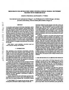
II. ESPRIT ALGORITHM Two different array antennas are considered in this paper, a square array with 9 elements and a honeycomb array with 19 elements. Array elements are uniformly placed on an x-y plane as shown in Figure 1. The inter-element spacing d equals half of the signal wavelength.
Index Terms—DOA estimation, array antenna, advanced signal processing.
I. INTRODUCTION Accurately estimating the direction of arrival (DOA) has many important applications in communication and radar systems. Using the conventional fixed antenna, the resolution of DOA is limited by the antenna mainlobe beamwidth. Using the array antenna and advanced signal processing techniques, the DOA estimation variance can be greatly reduced. Two important classes of signal processing techniques are the model based approach and the eigen-analysis method[1]. The model based method assumes that the received data is modeled as the output of a linear shift invariant system. The DOA information can be obtained indirectly from the estimated model parameters. Several eigen-analysis methods such as multiple signal classification (MUSIC)[2], root MUSIC[3,4], polynomial root intersection for multi-dimensional estimation (PRIME)[5,6] have been investigated by many authors. This paper studies DOA finding using estimation signal parameter via a rotational invariant technique (ESPRIT)[7]. Two different array antennas are used in this simulation study. In this paper DOA performance is discussed as a function of signal to noise ratio Manuscript received July 16, 2009. This work was supported in part by the Raytheon Space and Airborne Systems. Z. Aliyazicioglu is with the Electrical and Computer Engineering Department, California State Polytechnic University, Pomona, CA 91768 USA, phone: 909-869-3667; fax: 909-869-4687; (e-mail: zaliyazici@ csupomona.edu). H. K. Hwang is with the Electrical and Computer Engineering Department, California State Polytechnic University, Pomona, CA 91768 USA phone: 909-869-2539; fax: 909-869-4687; (e-mail:
[email protected]). Jose Bermudez, Ridwan C. Chin, Payam Davoodian, and Alfred Tsz Yin Lok are graduate students at the Electrical and Computer Engineering Department, California State Polytechnic University, Pomona, CA 91768.
ISBN:978-988-17012-6-8
Figure 1 Two Dimensional Arrays with 9 and 19 Elements
Assume a narrowband signal impinging on the array from an elevation angle θ and azimuth angle φ as shown in Figure 2. Using the signal received by the center element sc(t) as the reference, the signal received by the ith element si(t) is
WCECS 2009
Proceedings of the World Congress on Engineering and Computer Science 2009 Vol I WCECS 2009, October 20-22, 2009, San Francisco, USA
⎡0 ⎢1 where Q = ⎢ ⎢0 ⎢ ⎣0
0 0 0 0
0 0 0 1
0⎤ 0⎥⎥ 0⎥ ⎥ 0⎦
Arranging the eigenvalues of matrix Ryy λ1, λ2, λ3, λ4 in 2
descending order, the noise variance σ w can be estimated by the following equation.
σ 2w = ( λ2 + λ3 + λ4)/3
Figure 2 Coordinate of array system and signal direction
si(t) = sc(t) e
jβ i
(1)
Define matrices Cyy and Cyz as 2
2
2π sinθ(x i cosφ + y i sinφ) λ
(2)
where (xi, yi) are the coordinates of the i element. Equation (2) shows that the signal DOA angles (θ, φ) are related to the electrical angle β. The ESPRIT algorithm derives the DOA angles from the phase factor β. Determining two angles (θ, φ) requires two different phase factors. Two independent phase factors can be derived from two independent position shifts. A brief description of ESPRIT using a 9 element square array is as follows: The waveform y received by the subset consists of elements (1, 2, 4, 5) and can be expressed as: y(n) = s5(n)s + [w1(n), w2(n), w4(n), w5(n)]T
(3)
where s5(n) is the signal received by center element, s = jβ
jβ
[ e 1 , e 2 , e 4 , 1]T, and wk(n) k = 1, 2, 4, 5 are the white noise received by the elements of this subset. The correlation matrix Ryy of this subset is 2
2
Ryy = E[yyH] = σ s ssH + σ w I 2
(4)
2
where σ s and σ w are the variance of signal and noise respectively. Shifting this subset horizontally to the right forms a new subset consisting of elements (2, 3, 5, 6). The received waveform of this new subset z(n) is
[
]
z (n) = e jβ 6 s 5 (n) e jβ1 , e jβ 2 , e jβ 4 ,1
T
(5)
Ryz = E[yz ] = σ e
jβ 6
2 w
ss + σ Q H
ssH
(9)
)ssH, thus λ = e
[
-jβ 6
]
is one
T
+ [w 4 (n), w 5 (n), w 7 (n), w 8 (n)]
T
(10)
The cross correlation matrix Ryv is 2
Ryv = E[yvH] = σ s e
⎡0 ⎢0 where Q1 = ⎢ ⎢1 ⎢ ⎣0
jβ 8
2
ssH + σ w Q1
(11)
0 0 0⎤ 0 0 0⎥⎥ 0 0 0⎥ ⎥ 1 0 0⎦
Define matrices Cyy and Cyv as: 2
2
Cyy = Ryy - σ w I = σ s ssH 2
Cyv = Ryv - σ w Q1 = σ s e 2
(6)
jβ 6
v(n) = e jβ8 s 5 (n) e jβ1 , e jβ 2 , e jβ 4 ,1
jβ 8
(12) jβ 8
ssH
(13)
)ssH, thus λ = e
-jβ8
is one of
the roots of det(Cyy – λ Cyv). The second phase factor β8 can be obtained by finding the root of det(Cyy – λ Cyv) closest to the unit circle. Since β6 = πsinθcosφ, β8 = -πsinθsinφ, DOA information can be obtained by solving e
ISBN:978-988-17012-6-8
jβ 6
(8)
of the roots of det(Cyy – λ Cyz). One phase factor β6 can be obtained by finding the root of det(Cyy – λ Cyz) closest to the unit circle. Forming subset (4, 5, 7, 8) by shifting the subset (1, 2, 4, 5) down by d, the second independent phase factor can be obtained. The received data vector of this subset v is:
Then Cyy – λCyv = σ s (1 - λ e
The cross correlation matrix Ryz is 2 s
Then Cyy – λCyz = σ s (1 - λ e
2
T
+ [w 2 (n), w 3 (n), w 5 (n), w 6 (n)] H
2
Cyz = Ryz - σ w Q = σ s e 2
th
jβ
2
Cyy = Ryy - σ w I = σ s ssH
where the electrical angle of the ith element βi is
βi =
(7)
jπsinθcosφ
= r1 = e
jα 1
where r1 is
WCECS 2009
Proceedings of the World Congress on Engineering and Computer Science 2009 Vol I WCECS 2009, October 20-22, 2009, San Francisco, USA
the root of det(Cyy – λ Cyz) closest to unit circle and
e
jα 2
-jπsinθsinφ
= r2 = e where r2 is the root of det(Cyy – λ Cyv) closest to unit circle. πsinθcosφ = α1
(14)
−πsinθsinφ = α2
(15)
The azimuth and elevation angles can be found from the following equations. -1
(16)
-1
(17)
φ = tan (-α2/α1) θ = sin (α1/πcosφ)
DOA information using the 19 element honeycomb array can be obtained in similar manner.
r14 (n) =
[
1 y 1 (n)y *4 (n) + y 2 (n)y *5 (n) + y 3 (n)y *6 (n) (21) 6 * * * + y 4 (n)y 7 (n) + y 5 (n)y 8 (n) + y 6 (n)y 9 (n)
]
[
1 y1 (n)y*5 (n) + y 2 (n)y*6 (n) + y 4 (n)y *8 (n) (22) 4 * + y 5 (n)y 9 (n)
r15 (n) =
]
[
1 y 2 (n)y*4 (n) + y 3 (n)y*5 (n) + y 5 (n)y*7 (n) 4 + y 6 (n)y*8 (n)
r24 (n) =
]
r25(n) = r14(n)
(24)
r45(n) = r12(n)
(25)
Elements of the cross-correlation matrices can be computed in a similar manner.
III. MATRIX ESTIMATION Section 2 shows that the DOA angles are derived from the auto-correlation and cross-correlation matrices. DOA performance depends on the accurate estimation of matrices Ryy, Ryz, Ryv. Elements of matrices are estimated from the received data y(n) = s(n) + w(n) where s(n) and w(n) are the signal and white noise of the received data. Three matrix estimation methods, (1) temporal averaging, (2) spatial smoothing, (3) temporal averaging and spatial smoothing, are described in this section[8].
C. Temporal Averaging and Spatial Smoothing Method This method combines spatial smoothing and temporal averaging. After estimating the matrix elements rij(n) from spatial smoothing, an estimated rij is obtained by further averaging over N snapshots according to the following equation. rij =
A. Temporal Averaging Method This method estimates the matrix element rij by averaging the products of data received by the ith and jth elements over N snapshots according to the following equation: N
rij =
1 y i (n)y *j (n) ∑ N n =1
(18)
B. Spatial Smoothing Method Since the number of elements in the array is larger than the size of the subset, instead of discarding the data from elements outside of the subset, those data can be used to improve the estimation of rij. For example, elements of the correlation matrix of square array for subset (1, 2, 4, 5) are computed from the following equations. r11(n) = r22 = r44 = r55 =
r12 (n) =
1 9 y i (n)y *i (n) ∑ 9 i =1
(19)
1 N ∑ rij (n) N n =1
[
]
(20)
(26)
IV. SIMULATION RESULTS Assume a tone signal impinging the array from azimuth angle φ = 60˚, and elevation angle θ = 30˚. The signal to noise ratio SNR = 10 dB. Using 4 element subset, Figure 3(a) shows the scatter plot based on 1000 independent simulations using the 9 element square array. The estimated 4 × 4 matrices are obtained by temporal averaging over only 32 snapshots. Most of the data points are centered on the true signal direction (30˚, 60˚). There are also points scattered over the other angles. With temporal averaging and spatial smoothing, Figure 3(b) shows an improved scatter plot where most of the data points are concentrated on (30˚, 60˚). The averaged estimated angle errors for (a) and (b) are 11.84˚ and 2.19˚, respectively. The estimated angle error ε is computed by the following equation. ε = cos-1( k • kˆ )
1 y 1 (n)y *2 (n) + y 2 (n)y *3 (n) + y 4 (n)y *5 (n) 6 + y 5 (n)y *6 (n) + y 7 (n)y *8 (n) + y 8 (n)y *9 (n)
ISBN:978-988-17012-6-8
(23)
(27)
where k is the signal direction vector and kˆ is the direction vector of the estimated DOA.
WCECS 2009
Proceedings of the World Congress on Engineering and Computer Science 2009 Vol I WCECS 2009, October 20-22, 2009, San Francisco, USA scatterplot
scatterplot
200
70
150
68 66
100
64 50
62
φ 0
φ
60 58
-50
56 -100
54 -150
0
10
20
30
40
50
60
70
80
52
90
θ
50 20
(a)
22
24
26
28
30
32
34
36
38
40
θ
scatterplot 200
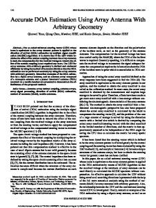
(b) Figure 4 Scatter Plots Based on 1000 Independent Simulations
150
100
50
φ
0
-50
-100 10
20
30
40
50
60
70
80
90
θ
(b) Figure 3 Scatter Plots Based on 1000 Independent Simulations
Figure 4 shows the scatter plots using a 19 element honeycomb array and 4 × 4 matrices. Figure 4(a) shows the scatter plot of 1000 independent simulations assuming SNR = 10 dB using temporal averaging over 32 snapshots. The result of the combination of temporal averaging and spatial smoothing is shown in Figure 4(b). The estimated angle errors are 12.98˚ and 0.97˚ for (a) and (b) respectively. Comparing Figures 3 and 4, the 19 element honeycomb array provides much better performance with special smoothing.
Increasing the number of temporal averaging improves DOA performance. Figure 5 shows the estimated angle error as a function of number of snapshots N using a 19 element honeycomb array. Increasing the number of temporal averaging improves the matrix element estimation; consequently the estimated angle error is reduced. The 19 element array provides sufficient number of spatial smoothing in matrix element estimation. The estimated angle error after spatial smoothing is considerably smaller than the estimated angle error without spatial smoothing. After spatial smoothing, temporal averaging over 200 snapshots provides a very good estimation. Further increasing the number of snapshots does not significantly reduce the estimation error. Estimated angle error vs. N 30
25
r or r e el g n a d et a m ti s E
before spatial smoothing after spatial smoothing
20
15
10
scatterplot 70
5 68 66
0
64
50
100
150 N
200
250
300
Figure 5 Estimated Angle Error as a Function of the Number of Temporal Averaging N
62
φ
0
60 58
Better SNR help improves the DOA performance. Figure 6 shows the estimated angle error using 19 element honeycomb array with N = 32.
56 54 52 50 20
22
24
26
28
30
32
34
36
38
40
θ
(a)
ISBN:978-988-17012-6-8
WCECS 2009
Proceedings of the World Congress on Engineering and Computer Science 2009 Vol I WCECS 2009, October 20-22, 2009, San Francisco, USA
estimation error whenever signal impinging the array from those special azimuth angles. Similarly, if 19 element array is used to estimate signal’s DOA, using the subset (1, 2, 4, 5) and shifting this subset to (2, 3, 5, 6) and (4, 5, 8, 9) would result a large estimated angle error the signal impinging the array from 90o, 270o, 150o and 330o.
Estimated angle error vs. SNR 35
30 without spatial smoothing with spatial smoothing
25 r or r e el g n a d et a m ti s E
20
Estimated Error Angle vs Azimuth Angle (Φ)(with Spaital Smoothing) 15
100 9-element Square 90
10
80
0
0
5
10
15
20 SNR(dB)
25
30
35
40
Figure 6 Estimated Angle Error as Function of SNR
With the elevation angle fixed at θ = 30o, Figure 7 shows that the estimation error is fairly independent of the azimuth angle. This result is based on using a 19 element array with SNR = 10 dB, temporal averaging over 32 snapshots; all matrices are 4 × 4. Figures 7 also indicate that estimation error can be reduced by an order of magnitude if the elements of matrix rij are estimated by spatial smoothing and temporal averaging methods. (a) 20 without spatial smoothing with spatial smoothing
16 14 r or r e e gl n a d et a m ti s E
12 10 8 6 4 2 0 -200
-150
-100
-50
0
50
100
150
200
φ
Figure 7 Estimated Angle Error as a Function of Elevation and Azimuth Angles
At high elevation angle, there are some special azimuth angles that yield a very large estimated angle error. The estimated angle error as a function of azimuth angles for 9 element arrays for signal impinging the array at high elevation angle (θ = 89o) is shown in Figure 8. This result is based on SNR = 10 dB and matrix elements are estimated by temporal averaging over 32 snapshots and spatial smoothing method. If the signal impinging the 9 element array from azimuth angle of 0o, 90o, 180o and 270o, the estimated angle error is very large. This is due to the fact that the received signal vectors of subset (1, 2, 4, 5) and subset (2, 3, 5, 6) are very close if the signal impinging the array from 90o or 270o. The received signal vector of subset (1, 2, 4, 5) and subset (4, 5, 7, 8) are very close if the signal impinging the array from 0o or 180o. The 9 element array produces very large
ISBN:978-988-17012-6-8
70 60 50 40 30 20 10 0
0
50
100
150
200
250
300
350
Φ (degree)
Figure 8 Estimated Angle Error vs Azimuth Angle for Elevation Angle θ = 89o V. CONCLUSION
Estimated angle error vs. Azimuth angle
18
Estimated Error Angles
5
The conclusions based on the results of this simulation study are summarized as follows: 1. The ESPRIT method estimates signal DOA by finding the roots of two independent equations closest to the unit circle. This method does not require using a scan vector to scan over all possible directions like the MUSIC (Multiple Signal Classification) algorithm. 2. Estimation error is relatively independent of signal azimuth angle if the signal impinging the array from low elevation angle. 3. When the signal impinging the array from high elevation angle, there are some critical azimuths angles that yield a very large estimation error. This is due to the fact that at those critical azimuth angles, the received data vectors are very close. Thus there is not sufficient information to process the received data. To avoid large estimation error, we suggest to alternatively choosing a different subset and shifting the subset in different directions. 4. Estimation error can be reduced by (a) using an array containing a large number of elements, (b) increasing the number of temporal averaging in matrix element estimation. 5. Array element position may deviate from the ideal position. Position deviation will degrade DOA performance. Sensitivity analysis due to imprecise element position will be carried out in future study. ACKNOWLEDGMENT The authors would like to thank the Raytheon Space and Airborne Systems for its support of this investigation.
WCECS 2009
Proceedings of the World Congress on Engineering and Computer Science 2009 Vol I WCECS 2009, October 20-22, 2009, San Francisco, USA
REFERENCES [1] [2] [3] [4] [5]
[6] [7] [8]
J. Proakis, D. K. Manolakis Digital Signal Processing, Prentice Hall, 2006, 4th Ed R.O Schmidt, "Multiple Emitter Location and Signal Parameter Estimation," IEEE Trans. Antennas Propagation, Vol. AP-34 M. Pesivento, A. B. Gershman, M. Haardt, “A Theoretical and Experimental Study of a Root MUSIC Algorithm based on a Real Valued Eigen decomposition” Z. Aliyazicioglu, H. K. Hwang, M. Grice, A. Yakovlev, ”Sensitivity Analysis for Direction of Arrival Estimation using a Root-MUSIC Algorithm” Engineering Letters, 16:3, EL_16_3_13 G. F. Hatke, K. W. Forsythe, “A class of polynomial rooting algorithms for joint azimuth/elevation estimation using multidimensional arrays” Signals, Systems and Computers, 1994. 1994 Conference Record of the Twenty-Eighth Asilomar Conference Z. Aliyazicioglu, H. K. Hwang, “Performance Analysis for DOA Estimation using the PRIME Algorithm” 10th International Conference on Signal and Image Processing, 2008 R. Roy, T. Kailath, “ESPRIT-estimation of signal parameters via rotational invariance techniques” IEEE Transactions on Acoustics, Speech and Signal Processing, 1989 S. Haykin, “Adaptive Filter Theory, Prentic Hall, 2002, 4th Ed”
ISBN:978-988-17012-6-8
WCECS 2009