In this paper the simulation decision-support tool for dynamic optimal dispatching ... dispatching control, decision support tools, simulation on-time service. 1.
Trmspn Res.-A, Vol. 32, No. 2, pp.7387, 1998
Pergnmon
All
SIMULATION DISPATCHING ANDRZEJ
0 1998ElsevierScience Ltd rights reserved. Printed in Great Britain 096%8564/98819.00+O.OO
SUPPORT TOOL FOR REAL-TIME CONTROL IN PUBLIC TRANSPORT ADAMSKI*
and ANDRZEJ TURNAU
Institute of Automatics, University of Mining and Metallurgy, 30-059 Cracow, Al. Mickiewicza 30/Bl, Poland (Received 21 July 1995; in revisedjorm 7 April 1997) Abstract-In practice punctuality of transit service has been a chronic operational problem mainly due to the random environment and very high complexity of the public transport processes. This challenging problem affects both travellers (reliability of service) as well as operators (productivity and efficiency of resources utilization). The potential of new information and communication technologies and existing hardware possibilities offer great opportunities for the development of effective and flexible management and control tools for public transport. In this paper the simulation decision-support tool for dynamic optimal dispatching control purposes have been developed, with the use of the SIMULINK package with Toolboxes. The following optimal dispatching control problems have been solved: punctuality control (which compensates deviations from schedule), regularity control (which compensates deviations from regular headway) and synchronizing control with linear (LQ, dead-beat) feedback and control and system state constraints; LQG stochastic control with real-time estimation of the model parameters; and bus route zone control for synchronising passenger transfers or the operation of different lines on common segments of the route. The results presented are illustrated by 15 numerical examples. 0 1998 Elsevier Science Ltd. All rights reserved Keywords: public transport, dispatching control, decision support tools, simulation on-time service
1. INTRODUCTION
Maintaining a scheduled reliable service for passengers in public transport is a key operational problem which affects both travellers and transit operators. The practical fulfilment of these service requirements is realized by transit planning and management action. It is a difficult task because public transport is a very complex system. The high complexity results from: 1. 2. 3. 4. 5.
the dynamics of traffic during the operation of vehicles on the routes; high level of demand and human behavioural uncertainty; unpredictable operational events and random disturbances (congestion blockades, accidents); unreliable operation of the driver-vehicle entity; and complex interactions with other vehicles, passengers demand and the environment (see Anderson et al., 1979; Adamski, 1980, 1989, 1992, 1993; Turnquist and Blume, 1980; Turnquist, 1982).
The minimum cost network flow problem is a typical operations research optimization model that is frequently used to assist decision makers in the areas of resource planning, scheduling and distribution. In public transport, this model is frequently used for problems such as service schedule and network route design. However, it is evident that due to the fixed demand assumption and the steady-state trip cost estimates, this model is not directly applicable to public transport. To overcome this difficulty, a new multilayer transit planning optimization problem was formulated (Adamski, 1993). The solution of this problem was split into the lower dispatching control layer, which realizes dynamic real-time schedule tracking control on the lines and provides for stable steady-state operation, and an optimization layer (optimizer) which solves the transit planning problem. The static approach to modelling makes possible effective use of feedback control.
*Author for correspondence. 73
A. Adamski and A. Turnau
14
At this point, it should be emphasized that the existence of effective real-time dynamic dispatching control (i.e. operating stability) which suppresses operating disturbances, deviations from schedule and transient effects on the lines, is a crucial condition of the practical adequacy of transit planning. A very important advantage which follows from the action of this dispatching control layer, results from the fact that for moderate and fast disturbances this layer may act autonomously, because in these cases the stabilization feedback is sufficient. This emphasizes, among others, the importance of distributed dispatching control (Adamski, 1989, 1993), realized practically by vehicles equipped with on-board computers. In practice, on real public transport lines, deviations from schedule, if not compensated for by dispatching control actions, are amplified by positive feedback mechanisms (e.g. the bunching phenomenon studied by Osuna and Newell, 1972; Newell, 1974; Adamski, 1980) and propagate along the route. The result is an increase in passenger trip and waiting times, transfer/arrival time uncertainty and uneven loads of the vehicles. One consequence is that poor-on-time service performance influences the choice of mass transit modes. This is why improvement of public transport services has received high attention in the literature. Previous research related to the use of simulation in public transport has been devoted to the creation of simulation models for the analysis of sources of service unreliability (Bly and Jackson, 1974; Jackson, 1977; Doras et al., 1978; Koffman, 1978; Anderson et al., 1979; Turnquist and Blume, 1980; Tumquist, 1982; Vanderbona and Richardson, 1986) and the evaluation of simple schedule-based or headway-based static control actions (e.g. holding, skipping, turning, rescheduling, reserve actuation) realized at selected points (checkpoints) on the route (Bly, 1974; Jackson, 1977; Doras et al., 1978; Koffman, 1978; Vanderbona and Richardson, 1986). Most of these evaluations dealt with simple holding strategies (Osuna and Newell, 1972; Newell, 1974; Barnett, 1974; Turnquist and Blume, 1980; Turnquist, 1982) and simulation attempts to optimize threshold value parameters with respect to average passenger waiting time. The general conclusion concerning the work may be summarized as follows: local control actions may be, to a high degree, profitable when they are properly co-ordinated and realized in the ‘control by opportunity’ mode i.e. at appropriate control points along the route based on the current system state. The difficulty lies in the identification of these control points. This is why a dynamic approach which integrates (in the time-space context) the simple control actions in an optimal dynamic control strategy seems to be a more natural approach. Previous dynamic approaches to dispatching control were concerned with the creation of dynamic, continuous- and discrete-time public transport line models, analytical solutions of small or aggregated dispatching control problems assigned to hierarchical and expert systems, numerical solutions of small dispatching control problems implemented in distributed control structures by on-board computers (Adamski, 1980, 1983, 1985, 1989, 1995a,b, 1996). In this paper the following tasks have been realized: 1. a simulation support tool for real-time dispatching control is developed on the basis of the SIMULINK package; 2. the application of this support tool is illustrated by a set of 15 new dispatching control verification examples; 3. a suboptimal real-time dispatching control algorithm, which is a modification of the Barr algorithm, has been proposed and illustrated in one numerical example; and 4. the destabilization effect due to time delays in the state variables for the bus route operated with an even number of buses has been illustrated in one example. In the next section a dynamic bus route punctuality model, which constitutes the base for dynamic dispatching control, is introduced and analysed. The two sections which follow deal with several dispatching control problems of practical importance which have been solved with the use of the SIMULINK package. 2. PUNCTUALITY
MODEL OF THE PUBLIC TRANSPORT LINE
We assume that the public transport line works in accordance with a fixed-schedule offering a high/medium service frequency. This schedule can be visually represented on a time-space plane by a set of planned vehicles trajectories [see Fig. l(a)]. Similarly, the executed service can be
Simulation support tool for public transport control
I
P
4
trah
---
intersection
Terminal 2
Terminal 1 Route I
P
b. Module-based bus line representation
Fig. 1. The bus line representations.
76
A. Adamski and A. Turnau
represented by a corresponding set of actual vehicle trajectories. As can be seen in Fig. 1 the pair of subscripts ‘iJ’ denotes the quantity connected with the ith vehicle at the jth point on the route (e.g. at a bus stop). Additionally, the superscript s denotes a schedule-related quantity e.g. 5 denotes scheduled departure time of the ith vehicle from the jth stop. Different route representations aggregated to route zones or modules, are also possible [see Fig. l(b)]. In general, the planned service differs from the executed service and a measure of this discrepancy can be used to represent this schedule deviation e.g. xij = tii - $ representing the schedule deviation expressed in terms of departure times. In the dynamic control model the interactions between the trafhc demand (i.e. passenger arrivals and service processes) and service supply (movement of vehicles) should be adequately represented. Therefore, a random passenger arrival pattern (perhaps non stationary) has been assumed with the estimated average passenger arrival rate hg. The most popular linear passenger dwell time model r = C + Kh (where r = stop time, C= dead time, h = service headway, K = ratio of average passenger arrival hu to boarding rate qt at bus stop) has been used (this is one from the family presented in Adamski, 1992). The service time in this model is dominated by the slowest stream of boarding passengers which is described by the average boarding time. From Fig. l(a) it can be seen that the stop time r~ of an ith vehicle atjth bus stop may be expressed either in terms of the traffic demand parameters [i.e. parameters of arriving and boarding streams of passengers, see left side of eqns (1) and (2)] or in terms of the parameters of the vehicle trajectories [see right side of eqns (1) and (2)]. Moreover, these expressions may be assigned to the executed (1) or planned (2) services. tij=Kii(tii-uii-tti-lj)+Cij+~ii=tij-T~ij-tii_l (1)
(2) where: rb denotes stop time including (C,, dead time, ti, passengers service time or layover times at terminals and uu the control decision time) tG/G denotes departure/schedule departure time of the ith vehicle from the jth stop (too = 0, td for j n, td = tmj-n due to periodicity of circulation of the vehicles). Similarly, tie for i m ta = ti, (the periodicity of the stops). T@/T; denotes vehicle travel/scheduled travel times spent travelling between j - 1 and j stops which may consist of delays in movement, time spent at intersections etc. KU = (lg/qu) E (0,l) and rg = 1 - KQ are the coefficients which when the schedule is adhered to ($j = 0), equalizes Ku = qj Denoting deviations from schedule of vehicle departure and trip times by x0 = tg - $ and .zg = Tu - T; + Cq - C$ respectively, according to eqn (1) and eqn (2) the following punctuality control model can be written in the vector notation form Xj+ 1 = /I; Xj +
AJ’xj-* + BjUj + A; Zj
(3)
where i= 1, .., m vehicle/j = 1, .., n of possible control points on a route indices xii-state variables representing deviations from schedule (xi E Rm) utl-control variables (uj E R’) zrf-disturbance variables representing deviations from schedule in travel times and driver behaviour (zj E R’) A; E Rmxm; Bj 5 Rmx’ are lower triangular diagonally dominated matrices with non-zero elements aik = hk nizk+t (1 - Al); b = a&k where xk = I/s are eigenvalues of matAx Ai. Al” E Rmxmis a matrix with non-zero elements in the last column equal to ch = ni=, (1 - A,) 2.1. Properties of the punctuality model 1. This linear non-stationary difference equation model, with delays in the state variables, can be transformed to the standard equivalent Frobenius form without delays (Adamski, 1983) by proper redefinition of the state variables.
Simulation support tool for public transport control
II
2. The uncontrolled system is structurally unstable in the Lapunov sense, which makes it possible to describe the well known vehicle bunching phenomenon observed in the operation of vehicles along the route (Fig. 2). The autonomous (i.e. time-invariant and uncontrolled) system has the following arrangement of eigenvalues: one multiple eigenvalue at the origin, one eigenvalue on the unit circle and the rest outside the unit circle. In the general case the instability results from the fact that the main diagonal of the first non-delayed part of the state equation dominates the delayed part (Adamski, 1983). Additionally, the destabilization effect of the delayed component Ayxj-, is observed when the bus route is operated with an even number of buses (see Fig. 17). Therefore in the cases when the schedule deviations can be spread to the new trips starting from the terminal, the odd number of buses is beneficial (see Fig. 18). The bunching phenomenon is the manifestation of the existence of positive feedback mechanism which amplifies the deviations from schedule of an off-schedule vehicle which propagates behind it (a directional characteristic) and affects all buses that follow. The odd spacing of the vehicles is enlarged by the odd service delay resulting from more/fewer passenger arrivals occurring during longer/shorter service intervals. The instability refers to the tendency for long/short intervals which become longer/shorter so that the vehicles tend to bunch and the passenger load is concentrated in the late vehicles. In consequence, the net effect of any deviation from schedule is the moving stable pair of vehicles formation. In the model the bunching directional characteristic is related to the lower triangular structure of the model matrices whereas the local bunching force range corresponds to the dominated diagonal of these matrices. 3. The regularity control model with the scheduled headway deviations hv = Hg - qj as state variables corresponds to the linear transformation of the state variables in the punctuality deviation [min]
10
r
.
Fig. 2. Uncontrolled bus schedule deviations (min).
Fig. 3. The illustration of the time sub-optimal procedure.
18
A. Adamski and A. Tumau
deviation [min]
1 2
Bus stop number
Fig. 4. Dead-beat with window t-2, O] for x6 State [min].
model hi, = XV -xi-y (i = 2,3, .., m) and hlj = Xlj - Xmj_n or in vector notation as hI = Pxj - et&,+ where in the matrix Z’(pii = 1, Ri+li = -1) and ei is the null vector with the ith element unity, the character ’ denotes transposition of vector e,,,. It can be therefore interpreted as an output equation in the punctuality model. As shown in Adamski (1983), the system is controllable for the bounded (to the polyhedron in Rm) disturbance vectors (i.e. any deviation from schedule xj # 0 may be compensated for in a finite interval by means of some control z+) and stabilizable i.e. all eigenvalues of the system may be transferred by means of closed-loop feedback into the unit circle, so that the system with feedback is stable. For the time-invariant case and non-constrained control, the state Xk = 0 may be reached in n steps. For the control constrained case, the system is controllable to some set. In this case, from the solution of the state equations and conditions of xj = 0, x0 # 0, )uj(O),the following equation x6 = QRU can be obtained where: QR = -[A;‘& A;*B, ., A;jB] is a mxj controllability matrix and u = [ua, ~1, .., uj-11 is the control vector. Using the concepi of minimal right pseudo inverse matrices, the control can be expressed as u = Qi [Q~Q’,] - x0 with ) uj ( UL&