A MATLAB Simulink-based simulator for an ... periences of using Simulink and
Lars Pettersson ...... for manner 1, the dummy bits of 'NULL' are padded to con-.
1
Simulink Based LTE System Simulator Master of Science Thesis in Communication Engineering
XUAN GUO & PENGTAO SONG Department of Signals and Systems CHALMERS UNIVERSITY OF TECHNOLOGY Göteborg, Sweden, 2010 Report No. EX097/2010
i
(This page is only for printing)
I
Simulink Based LTE System Simulator
Author Xuan Guo and Pengtao Song Master of Science thesis at Chalmers University of Technology in collaboration with Antenna Research Center, Ericsson Research.
Supervisor Mats Viberg, Chalmers Henrik Sahlin, Ericsson AB Patrik Persson, Ericsson AB
II
Simulink Based LTE System Simulator XUAN GUO & PENGTAO SONG
© XUAN GUO & PENGTAO SONG, 2010.
Technical report no EX097/2010 Department of Signals and Systems Chalmers University of Technology SE-412 96 Göteborg Sweden Telephone: + 46 (0)31-772 1000
Cover: A 3D graph showing the structure of the LTE dowlink simulator, according to Figure 4.1.
Göteborg, Sweden, 2010
III
Abstract A MATLAB Simulink-based simulator for an antenna system has been developed at Chalmers, followed by the implementation of a WCDMA system in it. Naturally, 3GPP LongTerm Evolution (LTE) as a new standard for communication system should be considered next. Therefore, a Simulink-based LTE system simulator connected to the existing antenna blocks and WINNER channel is presented in this master thesis. It focuses on the implementation of the LTE downlink in the physical layer. In the transmitter, functionalities like Turbo coding, rate-matching, MIMO (up to 4×4) and OFDM are realized. In the receiver, ideal and non-ideal receiver algorithms are supported, including two types of channel estimation, linear equalizer, Turbo decoding, PMI calculation and HARQ functionality. The results, such as raw bit error rate, bit error rate, block error rate and user throughput are studied in the simulator for different system settings. Keywords: Simulator, LTE, downlink, Simulink, WINNER, antenna, MIMO, Turbo coding, channel estimation, PMI
IV
Acknowledgements We are very grateful to our supervisors Mats Viberg at Chalmers, Henrik Sahlin and Patrik Persson at Ericsson. We express our special thanks to Henrik Sahlin and Patrik Persson who always give us patient helps whenever we are in trouble. We also have learnt a great deal from them. Ulf Carlberg also provided precious experiences of using Simulink and Lars Pettersson gave us useful explanations of the WINNER channel: many thanks to them too.
Xuan Guo and Pengtao Song Göteborg, Sweden, 2010
V
Contents LIST OF FIGURES ............................................ I LIST OF TABLES ............................................. II LIST OF ACRONYMS ..................................... III 1 1.1 1.2 1.3 1.4
INTRODUCTION ................................. 1 Background ....................................... 1 Scope of the thesis............................ 1 Outline of the report .......................... 1 Others.................................................2
2 2.1 2.2 2.3
PLATFORM: MATLAB SIMULINK ..... 3 Pre-defined blocks ............................ 3 Embedded MATLAB function ........... 4 Some Simulink tips ........................... 5
3 3.1 3.2 3.2.1 3.2.2 3.2.3 3.2.4 3.2.5 3.2.6 3.3 3.4 3.4.1 3.4.2 3.4.3 3.4.4 3.4.5 3.4.6 3.4.7
LTE DOWNLINK SIMULATOR ........... 7 Basic structure .................................. 7 Transmitter......................................... 7 Resource ............................................. 9 Channel coding ................................... 9 Rate-matching ................................... 14 Modulation ......................................... 18 Antenna mapping .............................. 19 Physical mapping .............................. 27 Channel Model ................................. 30 Receiver ........................................... 32 Channel estimation ............................ 33 Equalizer ........................................... 30 Pre-coding Matrix Indicator calculation .......................................................... 44 Demodulation .................................... 46 Inverse rate-matching ........................ 48 Channel decoding ............................. 49 Hybrid ARQ ....................................... 53
4 4.1 4.2 4.3 4.4
RUNNING THE LTE SIMULATOR .... 58 Name and functionality ................... 58 Usage ............................................... 61 Set up LTE downlink simulator ...... 62 Connect with new antenna blocks . 66
5
SIMULATION RESULTS................... 68
6
CONCLUSIONS AND FUTURE WORK .......................................................... 72
REFERENCES ............................................... 73
i
List of Figures FIGURE 3.1 THE STRUCTURE OF THE LTE SIMULATOR TRANSMITTER. .................. 8 FIGURE 3.2 THE CRC INSERTION OF ‘GCRC24A’ AND ‘GCRC24B'. ......................... 10 FIGURE 3.3 THE SIMULINK BLOCK OF GENERAL CRC GENERATOR. .................... 10 FIGURE 3.4 THE STRUCTURE OF THE TURBO ENCODER (DOTTED LINES APPLY FOR TRELLIS TERMINATION ONLY). .................................................................... 11 FIGURE 3.5 THE STRUCTURE OF TURBO CODING IN THE LTE SIMULATOR. ....... 12 FIGURE 3.6 SETTING PARAMETERS OF THE CONVOLUTIONAL ENCODER BLOCK IN THE LTE SIMULATOR. ........................................................................................ 13 FIGURE 3.7 CIRCULAR BUFFER WORK WITH PUNCTURING SCHEME................... 16 FIGURE 3.8 CIRCULAR BUFFER WORK WITH REPEATING SCHEME. ..................... 17 FIGURE 3.9 THE CONFIGURATION OF THE RECTANGULAR QAM MODULATOR BASEBAND BLOCK. ................................................................................................. 18 FIGURE 3.10 THE STRUCTURE OF ANTENNA MAPPING. .......................................... 19 FIGURE 3.11 LAYER MAPPING FOR SPATIAL MULTIPLEXING. ................................ 21 FIGURE 3.12 LAYER MAPPING FOR TRANSMIT DIVERSITY. ..................................... 22 FIGURE 3.13 THE PRE-CODING OF LARGER DELAY CDD. ....................................... 25 FIGURE 3.14 THE PRE-CODING OF LTE TRANSMIT DIVERSITY. .............................. 27 FIGURE 3.15 THE STRUCTURE OF OFDM MODULATION. ........................................ 30 FIGURE 3.16 ZERO PADDING OF OFDM MODULATION. .......................................... 30 FIGURE 3.17 THE STRUCTURE OF THE LTE SIMULATOR RECEIVER. ..................... 33 FIGURE 3.18 THE STRUCTURE OF IDEAL CHANNEL ESTIMATION. ........................ 34 FIGURE 3.19 THE STRUCTURE OF THE LEAST SQUARE ESTIMATOR. .................... 36 FIGURE 3.20 THE STRUCTURE OF THE MODIFIED LEAST SQUARE ESTIMATOR. 36 FIGURE 3.21 THE SIGNALS AT THE DIFFERENT STEPS OF A MODIFIED LEAST SQUARE ESTIMATOR. ............................................................................................. 38 FIGURE 3.22 THE CHANNEL ESTIMATION ON THE EDGE SYMBOLS. ..................... 39 FIGURE 3.23 THE DIALOG BLOCK OF THE BUFFER ................................................. 40 FIGURE 3.24 THE MODEL OF THE EQUALIZER. ......................................................... 40 FIGURE 3.25 THE CONFIGURATION OF THE RECTANGULAR QAM DEMODULATOR BASEBAND BLOCK. ................................................................... 47 FIGURE 3.26 THE STRUCTURE OF THE SISO BASED TURBO DECODER . .............. 50 FIGURE 3.27 THE STRUCTURE OF THE TURBO DECODING IN LTE SIMULATOR. 51 FIGURE 3.28 THE STRUCTURE OF ONE TURBO DECODING ITERATION UNIT BLOCK. ...................................................................................................................... 52 FIGURE 3.29 THE GENERAL CRC SYNDROME DETECTOR BLOCK IN SIMULINK.. 52 FIGURE 3.30 THE STRUCTURE OF HARQ IN THE SIMULATOR................................. 56 FIGURE 3.31 THE HARQ PROCESSES OF THE SIMULATOR (QPSK). ........................ 57 FIGURE 4.1 THE LTE DOWNLINK SIMULATOR............................................................ 59 FIGURE 4.2 THE DIALOG BLOCK OF THE ENODEB CONFIGURATION. ................. 63 FIGURE 4.3 THE DIALOG BLOCK OF THE UE CONFIGURATION............................. 65 FIGURE 5.1 THE RAW BER AND CODED BER FOR DIFFERENT MODULATIONS, WITH SISO TRANSMISSION MODE AND IDEAL CHANNEL ESTIMATION. ....... 69 FIGURE 5.2 THE THROUGHPUT BEFORE AND AFTER HARQ, WITH SISO TRANSMISSION MODE AND IDEAL CHANNEL ESTIMATION MODE. ............... 69 FIGURE 5.3 THE RAW BER FOR DIFFERENT CHANNEL ESTIMATION MODES. ..... 70 FIGURE 5.4 THE RAW BER WITH DIFFERENT TRANSMISSION MODES. .................. 71 FIGURE 5.5 THE THROUGHPUT BEFORE AND AFTER HARQ WITH DIFFERENT TRANSMISSION MODES. ......................................................................................... 71
ii
List of Tables TABLE 2.1 USED SIMULINK BLOCKS IN THE SIMULATOR. ........................................ 4 TABLE 2.2 SUPPORTED AND UNSUPPORTED MATLAB LANGUAGE FEATURES IN THE EMBEDDED MATLAB........................................................................................ 5 TABLE 3.1 THE VARIABLES OF PERMUTATION SEQUENCE FOR THE SUB-BLOCK INTERLEAVER IN THE LTE SIMULATOR. ............................................................. 14 TABLE 3.2 THE VARIABLES OF THE CIRCULAR BUFFER. ........................................ 17 TABLE 3.3 PARAMETERS FOR RECTANGULAR QAM MODULATOR BASEBAND. ... 18 TABLE 3.4 THE PARAMETERS OF THE ANTENNA MAPPING. ................................... 20 TABLE 3.5 TRANSMISSION MODE OF PDSCH. ............................................................ 22 TABLE 3.6 CODEBOOK FOR PRE-CODER MATRICES ON TWO ANTENNA PORTS. 23 TABLE 3.7 CODEBOOK FOR PRE-CODER MATRICES ON FOUR ANTENNA PORTS. .................................................................................................................................... 24 TABLE 3.8 MATRICES OF LARGE DELAY CDD. ........................................................... 26 TABLE 3.9 CONFIGURATION OF RESOURCE GRID IN THE LTE SIMULATOR. ...... 28 TABLE 3.10 DOWNLINK OFDM PARAMETERS. ........................................................... 29 TABLE 3.11 PRECODING MATRIX INDICATOR (PMI) DEFINITION ......................... 46 TABLE 3.12 PARAMETERS IN THE IMPLEMENTATION OF HARQ. ........................... 54 TABLE 4.1 THE NAME AND THE FUNCTIONALITY OF MAIN COMPONENTS. ........ 60 TABLE 4.2 THE MODIFIABLE PARAMETERS OF ENODEB. ....................................... 63 TABLE 4.3 THE MODIFIABLE PARAMETERS OF THE UE .......................................... 65 TABLE 4.4 THE MODIFIABLE PARAMETERS AT THE M-FILE OF ‘LTE_INITIALIZE.M’. ............................................................................................... 66 TABLE 4.5 THE INPUT AND OUTPUT DATA STRUCTURE OF ANTENNA BLOCKS . 67 TABLE 5.1 THE BASIC CONFIGURATIONS OF LTE SYSTEM FOR ALL SCENARIOS. .................................................................................................................................... 68
iii
List of Acronyms 3GPP ACK ARQ AWGN BCH BER BLER BPSK CDD CP CQI CRC CSI DCI DFT DL eNodeB FDD FFT FIR FSTD HARQ IDFT ISI LMMSE LTE MAC MIMO MRC OFDM PCCC PDCCH PDSCH PHY PMI PRB QAM QPSK RB RI RS RV RRT SFBC SINR SISO SNR TBS TTI
Third Generation Partnership Project Acknowledgement (in ARQ protocols) Automatic Repeat-reQuest Additive White Gaussian Noise Broadcast Channel Bit-Error Rate Block-Error Rate Binary Phase-Shift Keying Cyclic-Delay Diversity Cyclic Prefix Channel Quality Indication Cyclic Redundancy Check Channel State Information Downlink Control Information Discrete Fourier Transform Downlink E-UTRAN NodeB Frequency Division Duplex Fast Fourier Transform Finite Impulse Response Frequency Shift Transmit Diversity Hybrid ARQ Inverse DFT Inter-Symbol Interference Linear Minimum Mean-Square Error Long Term Evolution Medium Access Control Multiple-Input Multiple-Output Maximum Ratio Combining Orthogonal Frequency-Division Multiplexing Parallel Concatenated Convolutional Code Physical downlink control channel Physical downlink shared channel Physical layer Pre-coding Matrix Indicator Physical Resource Block Quadrature Amplitude Modulation Quadrature Phase-Shift Keying Resource Block Rank Indicator Reference Symbol Redundancy Version Round Trip Time Space Frequency Block Coding Signal-to-Interference plus Noise Ratio Single-Input Single-Output Signal-to-Noise Ratio Transport Block Size Transmission Time Interval
1
1
Introduction
1.1
Background An antenna system simulator based on Simulink has been developed by the Chase and Charmant research centers at Chalmers, followed by the implementation of a WCDMA system as a standard in 3G. LTE (Long Term Evolution), as an important technique of 4G, is naturally the task of the next stage. LTE can provide high data rates, low latency and flexible bandwidth. To achieve these targets, Orthogonal Frequency Division Multiplexing (OFDM) and Multiple-Input and MultipleOutput (MIMO) are adopted as basic technologies. Besides, other technologies like robust channel coding, scheduling, link adaptation and hybrid ARQ are also important.
1.2
Scope of the thesis First of all, it is necessary to present the scope of the thesis, including the requirements and some constraints on the implementation of the LTE system. • The implementation is based on the LTE Release 9 of the 3GPP specification. • The platform is MATLAB Simulink 7.5. • Only considered is the LTE downlink built between 1 base station (eNodeB) and 1 user equipment (UE). • The focus is mainly on the physical layer and partly on the MAC layer. • Only PDSCH (Physical Downlink Shared Channel) is considered and no control channels are considered. • Only FDD (Frequency-Division Duplexing) is supported. • The LTE system needs to be connected to the existing antenna blocks and the WINNER channel. Thus, this thesis focuses on the implementation of the transmitter and the receiver in LTE downlink, which are also the key content of this report. As for the WINNER channel and the antenna blocks, no more details will be included in this report. See references [1-3].
1.3
Outline of the report The report is organized as follows:
2
Chapter 2 gives a brief description of the MATLAB Simulink. In Chapter 3, the components of the transmitter and the receiver of LTE downlink are discussed in details. Chapter 4 describes how to set parameters and run the simulator. The results for different system settings are presented in Chapter 5. In the end, the work of the thesis is summarized and suggestions for future work are given in Chapter 6.
1.4
Others Some notations are explained in this Section in order to make the report more readable. Italic letter ( x ) denotes a variable. Lowercase letter in bold type ( x ) denotes a vector while uppercase letter in bold type ( X ) denotes a matrix. The transpose of vector x (or matrix X ) is expressed as x T (or X T ) while the conjugate transpose is expressed as x ∗ / x H (or X ∗ / X H ).
3
2
Platform: MATLAB Simulink The platform of the simulator is Simulink version 7.5, as one part of Release 2010a from the MathWorks. Simulink is well integrated with the MATLAB environment, which means Simulink has good access to many MATLAB features. Simulink is a software tool to model, simulate and analyze dynamic systems including signal processing, communication systems and control systems [4]. A feature of Simulink is that it is model-based. For modeling, a graphical user interface (GUI) is provided to hierarchically build models as blocks, which can be selected from existing predefined blocks or created according to the user’s wishes. To do a simulation, the Simulink menus or the command line in the MATLAB Command Window can be used. When analyzing, a large number of model analysis tools are available in both Simulink and MATLAB. In Simulink, the functions are performed by the blocks and the data can be transmitted between the blocks by the connecting lines, which represent the signals. The implementation of the blocks is a key step in the realization of this LTE system simulator. Next we will focus on the usage of pre-defined blocks, as well as building user-defined blocks.
2.1
Pre-defined blocks After typing ‘ simulink ’ in the command line of MATLAB Command Window, we can find the blocks. Simulink contains 16 standard block libraries, such as Commonly Used Blocks, Math Operations, Ports & Subsystems, Sinks, Sources, User-Defined Functions, etc. Except the library of User-Defined Functions, the libraries provide extensive blocks with different functions, which can be used directly. Besides, Simulink also includes several useful blocksets like Communications Blockset and Signal Processing Blockset. Besides, Simulink can also use some MATLAB toolboxes like Control System Toolbox. Mainly used in the simulator are the standard block libraries and the two blocksets. For the user’s convenience, some main blocks are listed in Table 2.1, together with their positions in Simulink (not including antenna parts). For more details, see the Product Help of MATLAB.
4
Pre-defined blocks can be directly used, which is the advantage of Simulink. However, as the practical requirements are far more complicated, it is impossible for these relatively simple blocks to model everything. That is why the embedded MATLAB function is introduced in the next section. Table 2.1 Used Simulink blocks in the simulator.
Blocks
Libraries
Switch
Commonly Used Blocks
For Each Subsystem
Ports & Subsystems
Selector Matrix Concatenate Delay Buffer
Signal Processing Blockset
Delay Line Frame Conversion General CRC Generator/syndrome detector Interlacer/Deinterlacer Convolutional Encoder APP Decoder Rectangular QAM Modulator/Demodulator Baseband
Communications Blockset
AWGN Channel Error Rate Calculation
2.2
Embedded MATLAB function There is an existing block named Embedded MATLAB function in the library of User-Defined Functions. Writing a MATLAB function in the block, you can create the model as you wish. In other words, embedded MATLAB function helps building custom models. Therefore, Embedded MATLAB function blocks are more flexible than the pre-defined blocks, despite the programming needed. In the simulator, more than half of the models are implemented using Embedded MATLAB function blocks, especially some key blocks like Precoding, Channel Estimation and Equalizer.
5
Nevertheless, an Embedded MATLAB function has limitations. Firstly, Embedded MATLAB is just a subset of the MATLAB language, which implies that it cannot support all the MATLAB language features. Table 2.2 shows several main supported and unsupported MATLAB language features in the Embedded MATLAB function (see more features in [5]). Secondly, for some MATLAB functions, there are also limitations. For example, the function fft / ifft in the Embedded MATLAB is only available when the length of the input vector is a power of 2. For the usage of randi , error , plot or disp , an extrinsic function declaration has to be made (see more limitations in Chapter 1 of [5]). Thirdly, before running a simulation, the Embedded MATLAB blocks need to generate efficient embeddable code via updating the Simulink diagram. This might take a significant amount of time for the first updating [6]. Table 2.2 Supported and Unsupported MATLAB language features in the Embedded MATLAB. N-dimensional arrays Matrix operations Variable-sized data Supported features
MATLAB program control statements if, switch, for, and while Subfunctions Persistent variables Global variables Structures Cell arrays Objects
Unsupported features
Nested functions Sparse matrices Try/catch statements Recursion
2.3
Some Simulink tips In this Section, we briefly talk about some main problems what we met during the work, as well as the solutions we used. a. Errors from some undefined variables in the Embedded MATLAB function
6
When the size of an undefined variable in the Embedded MATLAB function changes dynamically, especially in the loops, there will be an error saying “Undefined function or variable '(name)'. The first assignment to a local variable determines its class”. The solution is to initialize the variable to its full size in the beginning of the Embedded MATLAB function. b. How to transmit a constant value from workspace to Embedded MATLAB function. The constant value that has been saved as a variable at MATLAB workspace can be used in an Embedded MATLAB function. At first the variable should be added to the input argument list of the function. Afterwards open the Tools menu in an Embedded MATLAB function and select the Edit Data/Ports. Find the corresponding constant and set the Scope in the General menu as Parameter. To avoid errors, uncheck the Tunable box. c. Call external MATLAB functions. As mentioned in Section 2.2, Embedded MATLAB function does not support some MATLAB functions, like randi , error , plot , disp , etc. However, they can be used after an extrinsic function declaration at the top of the Embedded MATLAB function using eml.extrinsic . d. Take care of buffer latency problems. When using Buffer blocks, latency may be introduced. The problem of latency is annoying. Zero-tasking latency is only available in some special cases. For most cases, try to avoid this problem or solve it in the following way. Firstly, use the function rebuffer_delay to calculate the delay in order to make the schedule of buffer output clear. Then set a persistent variable to assist with the processing of output data in different time.
7
3
LTE downlink simulator
3.1
Basic structure The LTE downlink simulator simulates the downlink communication from one E-UTRAN NodeB (eNodeB) to one User Equipment (UE) using a WINNER channel or an AWGN channel. There are four main parts of the simulator: transmitter (eNodeB), channel, receiver (UE) and finally the outputs are calculated in one part. Note that the Chase Antenna blocks which were developed at Chalmers are connected with the simulator. The LTE downlink simulator is mainly modeled in the physical layer and partly in the Medium Access Control (MAC) layer. In terms of physical channel, the simulator focuses on the Physical Downlink Shared Channel (PDSCH). Moreover, the simulator operates in terms of sub-frames, i.e. the generation and transmission of signals are in the form of sub-frames.
3.2
Transmitter The transmitter in the physical layer starts with the grouped resource data which are in the form of transport blocks (see Figure 3.1). In each TTI, one transport block will be transferred first to the channel coding part which consists of two CRC encoders and one Turbo encoder. Then the block of the coded bits is named as a code block. The rate-matching block which cooperates with Hybrid ARQ is a kind of rate coordinator between the channel coding and the following blocks. In addition, since only one eNodeB is simulated, the scrambling process after rate-matching is neglected in the simulator. As illustrated in Figure 3.1, there are two process lines before the layer mapping block. The two lines correspond to the parallel processing of two codewords 1 in the case of spatial multiplexing transmission. Otherwise only one process line works. The layer mapping and precoding combined with different transmit schemes are two key approaches to achieve the MIMO functionality in LTE. Both of them are contained in the antenna mapping block of the LTE simulator.
1
A codeword is the block of the complex-valued modulation symbols. One codeword is defined per transport block.
Transmit Antenna OFDM
Rate Matching & HARQ
Physical Resource Mapping
Turbo Coding nd
Precoding
2 CRC Encoder
Modulation Mapping
…
Modulation Mapping
Layer Mapping
Segmentation st
1 CRC Encoder Transport Block 2
Transport Block 1
st
1 CRC Encoder
Segmentation
nd
2 CRC Encoder
Turbo Coding
Rate Matching & HARQ
…
8
Figure 3.1 The structure of the LTE simulator transmitter.
The following physical resource-mapping block and OFDM block are defined at each antenna port. They mainly arrange the transmitted symbols into a certain sub-carrier and time. In the end, the data will be transmitted to the WINNER channel through the transmit antennas.
9
Moreover, as the transmitter is specified in the 3GPP LTE specifications, it has been mainly implemented as in the specification unless stated otherwise. 3.2.1
Resource The transport channel is the interface between the physical layer and the MAC layer. As the LTE simulator focuses on the physical layer, the initial data is generated in the form of transport blocks. In the simulator, the resource generation is combined with the HARQ, which implies there will be two cases of resource generations. One is the generation of bits for a new transport block. The other is the retransmission of bits for the previous transport block, directly extracted from the buffer ‘ pers_ HARQprocessMat ’ (see Section 3.4.7). In the case of single-antenna transmission mode, there is only one transport block to be generated at each TTI. In the spatial multiplexing transmission mode, the simulator can run with up to two transport blocks at the same time. If there are two transport blocks, their transmissions or retransmissions are processed individually. Another important thing is the transport block size (TBS). It is decided by the number of Physical Resource Blocks (PRB) and the Modulation and Coding Scheme (MCS) from the MAC layer scheduler. The value of TBS is calculated in the initialization of the simulator.
3.2.2
Channel coding
3.2.2.1
Cyclic Redundancy Check According to [8], an encoder of Cyclic Redundancy Check (CRC) is utilized at the beginning of channel coding. There are two CRC schemes for PDSCH: ‘gCRC24A’ and ‘gCRC24B’ (see Figure 3.2). Both of them possess a 24 parity bits length, but work with different cyclic generator polynomials. The ‘gCRC24A’ focuses on a transport block, while the ‘gCRC24B’ focuses on the code block, which is a segmentation of a transport block when the size of a transport block is larger than the upper limit (6144 bits).
10
Transport block
Transport block
Total size>6144
gCRC24A
Code block 1 gCRC24B Code block 2 Figure 3.2 The CRC insertion of ‘gCRC24A’ and ‘gCRC24B'.
gCRC24B
For both schemes, the LTE simulator directly uses the General CRC Generator (see Figure 3.3) from the Simulink block library. The main parameters associated to this block are the ‘generator polynomial’ and the ‘checksums per frame’.
Figure 3.3 The Simulink block of General CRC Generator.
The ‘generator polynomial’ is specified as an integer row vector, containing the powers of nonzero terms in the polynomial. According to Section 5.1.1 in [8], the ‘gCRC24A’ and ‘gCRC24B’ work with the row vectors A and B respectively, which are written as A = [24, 23, 18, 17, 14, 11, 10, 7, 6, 5, 4, 3, 1, 0] ,
(3.1)
B = [24, 23, 6, 5, 1, 0] .
(3.2)
The default value of ‘checksums per frame’ is set to ‘1’ for both ‘gCRC24A’ and ‘gCRC24B’. This is due to the fact that, in each TTI, the input units of ‘gCRC24A’ and ‘gCRC24B’ are defined as 1 transport block and 1 code block respectively. Moreover, the encoding should be performed in a systematic form (that is, the original data bits appear at the front of the outputs). Such form is automatically generated by the General CRC Generator block. In Simulink the ‘For Each Subsystem’ block can achieve ‘for loop’ functionality. Thus it is applied to attach a ‘gCRC24B’ to each code block within one TTI.
11
3.2.2.2
Turbo encoder The channel coding scheme for PDSCH adopts Turbo coding, which is a kind of robust channel coding. When using an AWGN channel, the performance of Turbo codes can be close to the theoretical Shannon capacity limits. According to Section 5.1.3.2 of [8], the scheme of the Turbo encoder is a Parallel Concatenated Convolutional Code (PCCC) with two 8-state constituent encoders and one Turbo code internal interleaver. The theoretical structure of a Turbo encoder is shown in Figure 3.4.
x
st
1 constituent encoder
z D
Turbo code internal interleaver
D
k
k
D
nd
2 constituent encoder
z'
k
D
D
D
x'
k
Figure 3.4 The structure of the Turbo encoder (dotted lines apply for trellis termination only).
The output from the Turbo encoder consists of three information bit streams with the same length K : •
Systematic bit stream;
( x k , k = 0,1,..., K − 1)
•
Parity bit stream;
( zk , k = 0,1,..., K − 1)
•
Interleaved parity bit stream. ( z' k , k = 0,1,..., K − 1)
Since the receiver also has the knowledge of the Turbo internal interleave sequence, the interleaved systematic bit stream X k' will not be transmitted to the receiver. But the data of X k' will be partly utilized at the step of trellis termination.
12
The tail bits are independently appended at the end of each information bit stream to clean up the memory of all registers, i.e. terminate the encoder trellis to a zero state. Generally, the length of the tail bits is equal to the number of registers in one constituent encoder (3 registers are used in one convolutional encoder in LTE). According to Section 5.1.3.2.2 of [8], the sequence of tail bits is rearranged, and 4 tail bits are attached after each information bit stream. Hence, the length of each bit stream becomes K + 4 . With the three information bit streams, the original Turbo coding rate is 1/3. However, after padding tail bits, the coding rate will decrease a bit. Furthermore, by puncturing or repeating the output of Turbo coding, it can accomplish an alterable channel coding rate under different scenarios. Such process is implemented by the circular buffer at the rate-matching block, and it will be introduced in Section 3.2.3. In the LTE simulator, the implementation of the Turbo coding can be seen in Figure 3.5. The Convolutional Encoder Block (from the Simulink block library) is the main component of Turbo encoder which accepts a polynomial description of a convolutional encoder.
Figure 3.5 The structure of Turbo coding in the LTE simulator.
13
Figure 3.6 Setting parameters of the Convolutional Encoder Block in the LTE simulator.
As shown in Figure 3.6, the parameter of ‘Trellis structure’ is used to configure the encoder. The ‘poly2trellis’ 1 is a MATLAB function which can create such trellis structure. To speed up the LTE simulator, the trellis structure is predefined as a MATLAB variable ‘ constDL_Turbo.trellis ’ and it is configured as poly 2 strellis(4, [13,15],13 ) .
(3.3)
The Pad Block is utilized to pad 3 zeros at the end of each original information bit stream which will be passed to the following convolutional encoder. With 3 padded zeros, all the three registers of one encoder will be correspondingly set to zeros, namely the trellis will be terminated with zero state. The sequence of the generated tail bits will be rearranged at the Tail Bits Rearrange block which is implemented by an Embedded MATLAB Function block. The Turbo code internal interleaver is accomplished by a Selector Block (from Simulink block library). According to Section 5.1.3.2.3 in [8], the permutation sequence is predefined as a vector named ‘ constDL_Turbo.pi ’.
1
The Matlab function ‘poly2strellis’ needs the Communications Toolbox at MATLAB.
14
Note that the Selector Block supports zero-based index mode which is convenient for the permutation. The Deinterlacer Block can separate the systematic and parity bits from the output of the convolutional encoder. 3.2.3
Rate-matching The main task of the rate-matching is to extract the exact set of bits to be transmitted within a given TTI [15]. In Section 5.1.4 of [8], the rate-matching for Turbo coded transport channels is defined per code block. For each code block, there are three basic steps composing a rate-matching: subblock interleaver, bit collection and bit selection. Finally, after the rate-matching, each individually processed code block has to be concatenated and transferred to a modulation mapping block.
3.2.3.1
Sub-block interleaver The sub-block interleaver is defined for each output stream from Turbo coding. The streams include a systematic bit stream, a parity bit stream and an interleaved parity stream. For the sub-block interleaver in the LTE simulator, it takes advantage of a Selector Block (as the Turbo coding internal interleaver) to implement the interleaver functionality. According to Section 5.1.4.1.1 in [8], the permutation sequence is predefined based on the different interleave manners. The systematic and the first parity bit streams work with manner 1, meanwhile the interleaved parity bit steam works with manner 2. The predefined variables of permutation sequence associating to manner 1 and 2 are shown in Table 3.1. Especially for manner 1, the dummy bits of ‘NULL’ are padded to construct a matrix. The ‘NULL’ bits will be punctured in the circular buffer block. Table 3.1 The variables of permutation sequence for the sub-block interleaver in the LTE simulator. Manner
3.2.3.2
Variable name
manner 1
constDL_RateM.subbl_interleaver_seq
manner 2
constDL_RateM.subbl_interleaver_Pi_k
Bit collection The bit collection step concatenates the three bit streams (the systematic bit stream, parity bit stream and interleaved parity stream) together according to Section 5.1.4.1.2 of [8].
15
In the LTE simulator, the bit collection is mainly achieved by an Interlacer Block and a Matrix Concatenate Block. The Interlacer Block primarily puts the parity bit stream and the interleaved parity bit stream together as a new bit stream. Meanwhile it arranges the bits from the former stream at the odd sequence and the bits from the latter stream at the even sequence. Afterwards the Matrix Concatenate Block concatenates the new bit stream and the former systematic bit stream together to create the input for the following circular buffer block. 3.2.3.3
Bit selection The bit selection extracts consecutive bits from the circular buffer to the extent that fits into the assigned physical resource [15]. Combined with the Turbo coding, the circular buffer can puncture or repeat the collected coded bits to achieve an alterable channel coding rate under different scenarios. a. Start point To enable the operation of Incremental Redundancy (IR) based HARQ in LTE, the rate-matching is expected to provide different subsets of the code block for different transmissions of a packet. Hence, the concept of Redundancy Version (RV) is derived [10]. In the LTE simulator, the value of RV will be assigned from the HARQ scheduler to each code block to specify a start point of extracting bits from a circular buffer. See more details about the HARQ in Section 3.4.7. In the case of the first transmission of each coded block (RV = 0), puncturing a small amount of systematic bits is proposed in [8] and [10]. Namely, instead of reading out data from the beginning of systematic bit stream, the output of the circular buffer starts from a specified point (see in Figure 3.7). In the case of HARQ retransmission, the starting point of extracting bits will be configured according to a specified RV (RV = 1, 2, 3).
16
Systematic bits stream start point The stop point of bit selection within the first transmission of a code block
The start point of bit selection within the first transmission of a code block RV=0
RV=3
RV=1
Parity bits stream start point RV=2
Figure 3.7 Circular buffer work with puncturing scheme.
b. Circular buffer length In Section 5.1.4.1.2 of [8], the circular buffer length depends on two factors: • the length of bit stream K W reading out from the bit collection; • the length of total number of soft channel bits which associates to the UE category defined in Section 4.1 of [11]. The LTE simulator assumes the UE always possesses a minimum capacity to receive the maximum number of DLSCH transport block bits within a TTI, so the circular buffer length is always equal to the K W . The length is predefined as that of a variable named ‘constDL_RateM_embed.N_cb’ in the LTE simulator. The variable associates to the parameter of N cb in Section 5.1.4.1.2 of [8]. c. Stop point The bit selection stop point E 1 is calculated based on the total number of bits G 2 that available for transmission of one transport block in PDSCH.
1 2
For the definition of ‘E’, see Section 5.1.4.1.2 of [8]. For the definition of ‘G’, see Section 5.1.4.1.2 of [8].
17
The different code blocks which are segmented from one transport block may have a different stop point E in the circular buffer. In the case that E is less than N cb , a puncturing scheme is applied to the circular buffer (as the blue arrow shown in Figure 3.7); whereas in the case when E is larger than N cb , a repeating bit selection happens and starts from the specific start point again (see Figure 3.8).
Systematic bits stream start point
The start point of bit selection within the first transmission of a code block RV=0
The stop point of bit selection within the first transmission of a code block
RV=3
RV=1
Parity bits stream start point RV=2
Figure 3.8 Circular buffer work with repeating scheme.
Moreover, the circular buffer of the LTE simulator is implemented by an Embedded MATLAB Function Block. Particularly, when puncturing the dummy bits ‘NULL’, which are generated by the sub-block interleaver, the locations of ‘NULL’ will be directly passed to the Inverse Rate-Matching Block at the receiver side. In practice, it should be well predefined at a receiver to accomplish a sub-block deinterleaver. The main associated variables of the circular buffer are listed in Table 3.2. Table 3.2 The variables of the circular buffer. Name
Associated variables
Number of code blocks
constDL_RateM_embed.C
Length of circular buffer
constDL_RateM_embed.N_cb
Start point of bit selection
Start
Stop point of bit selection
constDL_RateM_embed.E
Note: the ‘constDL_RateM_embed.E’ is defined as a row vector, and the number of elements is equal to ‘constDL_RateM_embed.C’. Each element defines the stop point of bit selection on each code block.
18
3.2.4
Modulation There are three modulation schemes for the PDSCH: QPSK, 16QAM and 64QAM. In the LTE simulator, the Simulink block of Rectangular QAM Modulator Baseband is utilized to achieve the whole QAM modulation schemes above and also the QPSK scheme. This is based on the fact that the QPSK possesses the same constellation mapping as 4QAM.
Figure 3.9 The configuration of the Rectangular QAM Modulator Baseband block.
Figure 3.9 shows the configuration of the Rectangular QAM Modulator Baseband Block, and the corresponding predefined basic parameters are listed in Table 3.3. Table 3.3 Parameters for Rectangular QAM Modulator Baseband. Parameters
QPSK
16QAM
64QAM
19 constDL_MD. mary_num
Modulation order
Constellation mapping
constDL_MD. const_map
Minimum distance
constDL_MD. mini_dist
2
[2,3,0,1]
2
3.2.5
Antenna mapping
3.2.5.1
Overview
4
6
[11, 10, 14, 15, 9, 8, 12, 13, 1, 0, 4, 5, 3, 2, 6, 7]
[47,46,42,43,59,58,62,63, 45,44,40,41,57,56,60,61, 37,36,32,33,49,48,52,53, 39,38,34,35,51,50,54,55, 7, 6, 2, 3,19,18,22,23, 5, 4, 0, 1,17,16,20,21, 13,12, 8, 9,25,24,28,29, 15,14,10,11,27,26,30,31]
2 / 10
2 / 42
Antenna mapping is the combination of layer mapping and pre-coding, which jointly process the modulation symbols for one or two codewords to make them transmit on different antenna ports. The structure of antenna mapping is illustrated in Figure 3.10. nlayer layers
1 or 2 codewords
c(i)
nap antenna ports
x(i)
Layer mapping
s(i)
Precoding
RI
PMI
Figure 3.10 The structure of antenna mapping.
In Table 3.4, some necessary parameters are listed. The symbols for codewords, layers and antenna ports can be individually expressed as c(i) = [c 0 (i ),..., c n
codeword
x(i) = [ x 0 (i ),..., x n s(i) = [s 0 (i ),..., s n
layer
ap
−1
−1
−1
codeword −1, (i )]T , i = 0,1,.., M symb
layer − 1, (i )]T , i = 0,1,.., M symb
ap −1. (i )]T , i = 0,1,.., M symb
20
Table 3.4 The parameters of the antenna mapping. Name
Description
Name in simulator
Transmission mode
MAC.TxMode
The number of codewords
MAC.num_codewords
The number of layers
MAC.num_layers
The number of antenna ports
(not used)
nTx
The number of transmit antennas
MAC.Tx_ANT.num
nRx
The number of receive antennas
MAC.Rx_ANT.num
The number of symbols per codeword
constDL_PRECOD. M_codeword _symb
TxMode n codeword
n layer nap
codword M symb
layer M symb
The number of symbols per layer
ap M symb
The number of symbols per antenna port
RI PMI
Rank Indicator, i.e. a recommended number of layers by UE Pre-coding Matrix Indicator, i.e. a recommended pre-coder matrix by UE
constDL_PRECOD. M_layer_symb constDL_PRECOD. M_ap_symb RI PMI
Note: 1. Because only cell-specific reference signals are temporarily taken into account, which means that no ports other than ports {0, 1, 2, 3} are considered, in the simulator n ap is equal to nTx, i.e. the number of transmit antennas (see more in page 326-327 of [15]). 2. In the simulator, the case of two codewords separately with different sizes is not included.
3.2.5.2
Layer mapping In the layer mapping, the modulation symbols for one or two codewords will be mapped onto one or several layers. According to Section 6.3.3 in [7], except the transmission on a single antenna port (in this case, the symbols for one codeword is directly mapped onto one layer), there are mainly two kinds of layer mapping: one for spatial multiplexing and the other for transmit diversity.
21
In case of spatial multiplexing, there may be one or two codewords. But the number of layers is restricted. On one hand, it should be equal to or more than the number of codewords. On the other hand, the number of layers cannot exceed the number of antenna ports. The most important thing is the concept of ‘layer’. The layers in spatial multiplexing have the same meaning as ‘streams’. They are used to transmit multiple data streams in parallel, so the number of layers here is often referred to as the transmission rank [15]. In spatial multiplexing, the number of layers may be adapted to the transmission rank, by means of the feedback of a Rank Indicator (RI) to the layer mapping, as Figure 3.10 shows. The implementation of layer mapping for spatial multiplexing is depicted in Figure 3.11. Note: 1. In this simulator, only a fixed number of layers is initialized and used. A RI is calculated in the receiver. However, it is not sent back. This calculation is only available for closedloop multiplexing. 2. Mapping two codewords onto three layers is not available, as the transmission of two transport blocks with different sizes are currently not supported by this simulator.
1 codeword
1 codeword
1 layer
2 layers
2 codewords
2 layers
2 codewords
4 layers
Figure 3.11 Layer mapping for spatial multiplexing.
22
In case of transmit diversity, there is only one codeword and the number of layers is equal to the number of antenna ports. Moreover, the number of layers in this case is not related to the transmission rank, because transmit-diversity schemes are always single-rank transmission schemes [15]. The layers in transmit diversity are used to conveniently carry out the following pre-coding by some pre-defined matrices. Figure 3.12 shows the implementation of layer mapping for transmit diversity. 1 codeword
1 codeword
2 layers
4 layers
Figure 3.12 Layer mapping for transmit diversity.
3.2.5.3
Pre-coding According to different transmission modes, symbols on each layer will be pre-coded for transmission on the antenna ports. Table 3.5 shows transmission modes for PDSCH [9], as well as the corresponding status in the simulator. Table 3.5 Transmission mode of PDSCH. Transmission Transmission scheme of PDSCH mode
Status
Mode 1
Single-antenna port; port 0
Supported
Mode 2
Transmit diversity
Supported
Mode 3
Large delay CDD
Supported
Mode 4
Closed-loop spatial multiplexing
Supported
Mode 5
Multi-user MIMO
Mode 6
Closed-loop spatial multiplexing using a single transmission layer
Mode 7
Single-antenna port; port 5
Not supported
Mode 8
Dual layer transmission; port 7 and 8 or single-antenna port; port 7 or 8
Not supported
Not supported Supported
Note: Only one user and only transmission using cell-specific reference signals are considered, so modes 5, 7, 8 are not supported.
23
3.2.5.3.1
Single-antenna port; port 0 This mode uses only one transmit antenna. In this case, there may be two or more receive antennas, which can configure receiver diversity. The pre-coding of this mode is defined by ap layer [7]. = M symb s 0 (i ) = x 0 (i ) and M symb
3.2.5.3.2
Closed-loop spatial multiplexing The pre-coding for closed-loop spatial multiplexing has a structure shown in Figure 3.10, with a feedback of PMI. It is defined by [7] (3.4)
s(i) = W(i)x(i) ,
where W(i) is the pre-coding matrix of size n ap × n layer and ap ap layer . i = 0,1,.., M symb − 1 , M symb = M symb
In this mode, the decision of W (i) should take into account the feedback of PMI. The relation between W(i) and PMI will be discussed in Section 3.4.3. In practice, the eNodeB may, or may not, use the recommended W(i) . For simplification, the eNodeB of the simulator directly follows the recommendation of the UE and all the symbols in a sub-frame are using the same W(i) , which implies that W(i) changes with subframe. According to the specification [7], there are two codebooks of the pre-coder matrices. One codebook is for two antenna ports and one and two layers, as illustrated in Table 3.6. The other codebook is for four antenna ports and one, two, three and four layers, as listed in Table 3.7. Both closed-loop spatial multiplexing and open-loop spatial multiplexing use these codebooks. Note that for all the transmission modes, the total power of the signals does not change after the implementation of pre-coding. Table 3.6 Codebook for pre-coder matrices on two antenna ports. Index 0 1 2 3
n layer 1
2
1 1 2 1
1 1 0 2 0 1 1 1 1 2 1 − 1
1 1 2 − 1 1 1 2 j 1 1 2 − j
1 1 1 2 j − j
24 Note: In case of closed-loop spatial multiplexing, the codebook index 0 is not used when the number of layers is two. Table 3.7 Codebook for pre-coder matrices on four antenna ports. Index
n layer
un 1
2
3
4
0
u 0 = [1 − 1 − 1 − 1]T
W0{1}
W0{14 }
2
W0{124 }
3
W0{1234 } 2
1
u1 = [1 − j − 1 j ]T
W1{1}
W1{12 }
2
W1{123 }
3
W1{1234 } 2
2
u 2 = [1 1 − 1 1]T
W2{1}
W2{12 }
2
W2{123 }
3
W2{ 3214 } 2
3
u 3 = [1 j 1 − j ]T
W3{1}
W3{12 }
2
W3{123 }
3
W3{ 3214 } 2
4
1 ( − 1 − ) 2 j u4 = −j (1 − j ) 2
W4{1}
W4{14 }
2
W4{124 }
3
W4{1234 } 2
W5{1}
W5{14 }
2
W5{124 }
3
W5{1234 } 2
W6{1}
W6{13 }
2
W6{134 }
3
W6{1324 } 2
W7{1}
W7{13 }
2
W7{134 }
3
W7{1324 } 2
5
6
7
1 (1 − j ) 2 u5 = j ( −1 − j ) 2 1 (1 + j ) 2 u6 = −j ( −1 + j ) 2 1 ( − 1 + ) 2 j u7 = j (1 + j ) 2
8
u 8 = [1 − 1 1 1]T
W8{1}
W8{12 }
2
W8{124 }
3
W8{1234 } 2
9
u 9 = [1 − j − 1 − j ]T
W9{1}
W9{14 }
2
W9{134 }
3
W9{1234 } 2
10
u10 = [1 1 1 − 1]T
W10{1}
{13 } W10
2
{123 } W10
3
{1324 } 2 W10
11
u11 = [1 j − 1 j ]T
W11{1}
{13 } W11
2
{134 } W11
3
{1324 } W11 2
12
u12 = [1 − 1 − 1 1]T
W12{1}
{12 } W12
2
{123 } W12
3
{1234 } W12 2
13
u13 = [1 − 1 1 − 1]T
W13{1}
{13 } W13
2
{123 } W13
3
{1324 } W13 2
14
u14 = [1 1 − 1 − 1]T
W14{1}
{13 } W14
2
{123 } W14
3
{ 3214 } W14 2
15
u15 = [1 1 1 1]T
W15{1}
{12 } W15
2
{123 } W15
3
{1234 } W15 2
Note: Wn{s } consists of the columns {s } of the matrix Wn , Wn = I − 2u n u Hn u Hn u n , where I is the 4 × 4 identity matrix.
25
3.2.5.3.3
Large delay CDD There is a delay for the feedback of PMI in closed loop spatial multiplexing. When the UE moves at a high speed, the channel changes fast and the PMI delay may be larger than the coherence time of the channel. So the feedback of PMI is not reasonable any more. In this case, large delay CDD, another name of open-loop spatial multiplexing, is adopted as a replacement [15]. It does not require feedback of the pre-coding matrix by the UE. Instead, it cyclically applies some predetermined matrices. n layer layers x(i)
n ap antenna ports s(i)
U
D(i)
W(i)
n layer × n layer
n layer × n layer
nap × nlayer
Figure 3.13 The pre-coding of larger delay CDD.
As seen in Figure 3.13, the pre-coding of larger delay CDD is defined by [15] s(i) = W(i)D(i)Ux(i) ,
(3.5)
ap ap layer . U is the DFT preWhere i = 0,1,.., M symb − 1 and M symb = M symb coding matrix [20] of size nlayer × nlayer and D(i) is a diagonal matrix of size nlayer × nlayer supporting cyclic delay diversity, listed in Table 3.8. The principle of CDD is explained in detail in [15-16]. Note that there is no matrix for a single layer, as larger delay CDD is only defined for the case of two or more layers [15].
The matrix W(i) is selected from the codebook in Table 3.6 or Table 3.7. For two antenna ports, W(i) is assigned as W(i) =
1 1 0 . 2 0 1
(3.6)
For four antenna ports, W(i) changes cyclically according to the index i , assigned as W(i) = C k ,
(3.7)
26
where k is the index given by k = ( i n layer mod 4 ) + 1 and C1, C 2 , C 3 , C 4 separately correspond to the matrices W12{ s } , W13{ s } , W14{ s } , W15{ s } in Table 3.7 (the set {s } is decided by the number of layers). Table 3.8 Matrices of Large delay CDD.
n layer 2
1 1 1 1 e − j 2π / 2 2
3
1 1 1 − j 2π / 3 1 e 3 − j 4π / 3 1 e
4
3.2.5.3.4
D(i)
U
1 1 − j 2π / 4 1 1 e 2 1 e − j 4π / 4 − j 6π / 4 1 e
0 1 0 e − j 2πi / 2
e e − j 8π / 3 1
0 1 − j 2πi / 3 0 e 0 0
1
− j 4π / 3
− j 4π / 4
e e − j 8π / 4 e − j 12π / 4
e e − j 12π / 4 e − j 18π / 4 1
− j 6π / 4
0 1 − j 2πi / 4 0 e 0 0 0 0
e − j 4πi / 3 0 0 0
0 e
− j 4πi / 4
0
− j 6πi / 4 e 0 0 0
Closed-loop spatial multiplexing using a single transmission layer This mode is a special case of closed-loop spatial multiplexing when the number of layers is one. It can be regarded as codebook-based beam-forming. In this case, a recommendation of pre-coding vector should also be reported by the UE. Similarly, the recommended vector is directly used by the eBodeB. The vector is selected from the codebook in Table 3.6 or Table 3.7, only for a single layer.
3.2.5.3.5
Transmit diversity Transmit diversity for two antenna ports is based on Space Frequency Block Coding (SFBC), and transmit diversity for four antenna ports is based on a combination of SFBC and Frequency Shift Transmit Diversity (FSTD) [15]. According to the specifications [7], transmit diversity is implemented by a pre-defined matrix. The functionalities for both two and four antenna ports are illustrated in Figure 3.14. It can be seen that compared with the case of two antenna ports, the fourantenna-port transmission has a reduced bandwidth utilizaap tion. Note that unlike spatial multiplexing, M symb in transmit codeword layer diversity equals M symb rather than M symb , which just implies that the concept of layers for the two cases are basically different.
27
Si , Si + 2 , ...
Si ,
Si +1, Si + 2 , Si + 3 , ...
Antenna port #0
Precoding
− Si∗+1, Si∗ , − Si∗+ 3 , Si∗+ 2 , ...
Si +1, Si + 3 , ...
Antenna port #1
a. 2-antenna-port transmit diversity.
S i , ...
Si ,
S i +1,
0,
0, ... Antenna port #0
S i +1, ...
0,
0,
S i + 2 , S i + 3 , ... Antenna port #1
Precoding
S i + 2 , ...
− S i∗+1, S i∗ ,
0,
S i + 3 , ...
0,
0,
0, ...
Antenna port #2
− S i∗+ 3 , S i∗+ 2 , ... Antenna port #3
b. 4-antenna-port transmit diversity. Figure 3.14 The Pre-coding of LTE transmit diversity.
3.2.6
Physical mapping
3.2.6.1
Resource mapping As defined in Section 6.2 of [7], the transmitted signal in each DL slot time is described by a resource grid of N RB N scRB subDL carriers and N symb OFDM symbols. In case of multi-antenna transmission, there is one resource grid defined per antenna port. Furthermore, each antenna port is defined by its associated reference signal. Each element in the resource grid for a specified antenna port is called a resource element, and is uniquely identified by the index pair (k, n) in a slot, where k and n are the indices in the frequency and time domains respectively.
The resource-mapping block maps data symbols, reference signal symbols and control information symbols into a certain resource element at different antenna ports.
28
In the LTE simulator, users can configure the properties of the resource grid with the parameters listed in Table 3.9. Since only a cell-specific reference signal is considered, the antenna ports associating to the LTE simulator contain antenna port 0-3 (defined in Section 6.10.1.2 of [7]). Table 3.9 Configuration of resource grid in the LTE simulator. Name
Associated parameters
Options
MAC.N_RB
6, 15, 25, 50, 100
Number of physical resource blocks ( nPRB )
MAC.N_PRB
1− 98
Cyclic Prefix type
MAC.CP.type
1 for normal CP 2 for extend CP
Number of OFDM symbols for L1/L2 control signals
MAC.control_region.size
0, 1, 2, 3, 4
Number of resource blocks ( NRB )
Note: 1. The number of resource blocks is defined for the LTE system, and it associates to the system bandwidth and sampling frequency. 2. The number of physical resource blocks is defined for one UE, and is associated to the bandwidth of the UE. 3. Although there is no PDCCH in the LTE simulator now, the resource elements for the L1/L2 control signals are preserved and set to 0.
On each antenna port, resource mapping is implemented separately. Particularly, a certain resource element used for reference signal transmission on one antenna port in a slot shall not be used for any transmission on other antenna ports in the same slot and is therefore set to 0. The implementation of resource mapping in the LTE simulator is done by Embedded MATLAB Function blocks. The reference signals are generated by a pseudo-random sequence generator. In the LTE simulator, to simplify the initialization of the generator, the slot number is defined from 0 to 1 (originally, 0-19 defined in the Section 6.10.1.1 of [7]), and the cell ID is defined as 0 for only one cell in the LTE simulator. 3.2.6.2
OFDM Orthogonal Frequency Division Multiplexing (OFDM) is a basic technology of LTE, which is used in the downlink transmission scheme. OFDM can be seen as a kind of multi-carrier modulation, which divides a large system bandwidth into multiple narrowband sub-carriers. This makes each sub-carrier nearly flat fading. The use of cyclic-prefix mitigates intersymbol interference in a time-dispersive channel.
29
The OFDM modulator can be implemented by a scaled inverse fast Fourier transform (IFFT), following the formula (3.1) in [18] x(n ) =
1
N −1
∑ X (k )e N
j 2πkn / N
, n = 1,2,..., N − 1 ,
(3.8)
k =0
where X (k ) is the discrete signal in the frequency domain, x (n ) is the discrete signal in the time domain and N is the FFT size. Correspondingly, the OFDM demodulator can be expressed as a scaled FFT, following the formula (3.2) in [18] N −1
X (k ) = N ∑ x (n )e − j 2πkn / N , k = 1,2,..., N − 1 .
(3.9)
n =0
There are several basic parameters of OFDM in this simulator, such as the sub-carrier spacing ( ∆f ), the number of subcarriers ( Nsc ), the cyclic prefix length ( Ncp ) and the FFT size ( N ). As shown in Table 3.10, a sub-carrier spacing of 15 kHz is used and the latter three parameters are decided by the system bandwidth ( BW ). There are also other related parameters in this table, like the sampling frequency ( fs ) and the number of OFDM symbols in a slot ( Nsymb ). The cyclic prefix length is specified in terms of samples, while in the specification [7], it is in terms of unit time. Note that a system bandwidth of 15 MHz is not available in this simulator, as embedded MATLAB function only supports radix-2 FFT. All other bandwidths in Table 3.10 are supported.
Table 3.10 Downlink OFDM parameters [7] [12].
BW (MHz)
1.4
3
∆f
5
10
15
20
15 kHz
Nsc
72
180
300
600
900
1200
N
128
256
512
1024
1536
2048
Sampling Rate
1.92
3.84
7.68
15.36
23.04
30.72
Nsymb Ncp
7/6 (normal/extended CP)
Normal
9 (10)
18 (20)
36 (40)
72 (80)
108 (120)
144 (160)
Extended
32
64
128
256
384
512
30
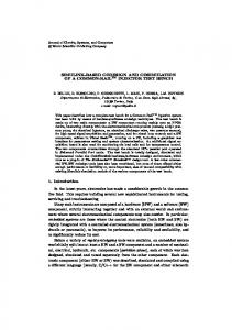
Frequency domain
Zero padding
Time domain
IFFT
CP insertion
Figure 3.15 The structure of OFDM modulation.
The structure of OFDM generation for each antenna port for is illustrated in Figure 3.15. The zero padding process is shown in Figure 3.16 (the first value after zero padding is an unused DC-sub-carrier and the blank part in the figure is padded with zeros). An IFFT transforms frequency-domain signals into time-domain signals, i.e. OFDM symbols. The CP insertion copies the last Ncp samples of the OFDM symbol and appends them at the beginning of the symbol. 1
Nsc/2
Nsc
Before:
After: 2
Nsc/2 + 1
N - Nsc/2 + 1
N
f
Figure 3.16 Zero padding of OFDM modulation.
In the implementation of OFDM, Embedded MATLAB function is used. The OFDM parameters have corresponding names to those stated in Table 3.10. Another parameter ‘ MAC.CP.type ’ is also set to specify a case of normal CP or extended CP (see Table 3.9).
3.3
Channel Model In the LTE simulator, two channel models are applied: a WINNER channel mode and an AWGN channel mode. The WINNER channel can provide a multi-path fading channel under different scenarios, and it can support the 2 × 3 MIMO functionality currently. In the LTE downlink simulator, the channel estimator will focus on each single channel path separately in the frequency domain. For convenience, we describe the channel from one transmit antenna to one receive antenna as a column vector
31
h = [H 0
H 1 H N −1 ]
T
(3.10)
in the frequency domain. Here, H j ( j = 0,1, N − 1 ) is the channel gain on each sub-carrier in the frequency domain; N is equal to the number of sub-carriers within all RBs. The path loss and channel fading are assumed to be included in h . In the case of MIMO transmission, each channel path h will be estimated at the receiver side. The transmitted signals can be expressed as a diagonal matrix
0 0 X1 0 0 X N −1
X0 0 X= 0
(3.11)
in the frequency domain. After the processing of inverse-OFDM on each receive antenna port, a received signal can be described as a column vector y with N elements, and y = Xh + v ,
(3.12) 1
h = Fg ,
(3.13)
where v is a vector of the noise in the frequency domain, g is a vector of the channel impulse response in the time domain, and W N00 F= ( N W N −1)0
W N0( N −1) W N( N −1)( N −1)
(3.14)
is the DFT-matrix with
W
nk N
=
1 N
e
− j 2π
nk N
.
(3.15)
In case of the AWGN channel mode, the h in Equation (3.12) is a column vector with N elements of 1.
1
As a matter of convenience, Equation (3.12) is written in a matrix notation.
32
In the LTE simulator, as a matter of convenience, the white noise v is directly added in the frequency domain (see the Note in Section 3.4.1.2). In addition, the Chase Antenna Blocks are not connected when using the AWGN channel mode.
3.4
Receiver In the LTE downlink simulator, the receiver side simulates the operation of one user equipment that processes the received signals and interacts with the eNodeB. Figure 3.17 shows the basic flow. After the steps of inverse-OFDM and inverse resource mapping, the receiver has to do the channel estimation to provide the necessary channel information to the following blocks of equalizer and PMI calculation. Note that after the layer extracting, up to two processing lines operates in parallel in case of spatial multiplexing. Otherwise there is only one process line in action. In each TTI, the following blocks of demodulation, inverse rate-matching, channel decoding, and HARQ will detect each transmitted bits and ask for a retransmission if any errors remain after the Turbo decoding. Finally, the PMI will be fed back to the eNodeB, and the decoded bits are transferred to the output calculation block to evaluate the simulator performance in each TTI. Because the receiver is not specified in the 3GPP specifications [7-9], this part is mainly implemented based on the books and articles from [19] to [27].
Figure 3.17 The structure of the LTE simulator receiver.
3.4.1
Channel estimation
3.4.1.1
Overview The main functionality of the channel estimation is to provide an estimated channel hˆ to the equalizer and the calculators of the RI and PMI in the frequency domain. A noise variance estimate is also provided from the channel estimation. For brevity, the description of the calculation for this noise variance is omitted.
HARQ
CRC Check Channel Decoding InverseRate Matching Soft Demodulation
…
PMI Calculation
Channel Decoding InverseRate Matching Soft Demodulation
Receive Antenna
InverseOFDM
InverseResource Mapping
Extract Reference Signals
Equalizer
Channel Estimation
CRC Check
Extract Layers
…
Outputs Calculation
33
34
In an LTE downlink system, the symbols of the reference signal are inserted within fixed sub-carriers per antenna port as defined in Section 6.10 of [7]. Thus, the preliminary step is to estimate a physical channel at the reference signals’ subcarrier frequency in the frequency domain and within each sub-frame in the time domain. After the preliminary channel estimate, based on the available channel information, an interpolation is applied to the other data symbols both in the frequency and time domain. In the LTE simulator, three channel estimation models are accomplished: • Ideal channel estimation with Least Square (LS) estimator; • Non-ideal channel estimation with LS estimator; • Non-ideal channel estimation with modified LS estimator. Section 3.4.1.2 describes the implementation of ideal channel estimation in the LTE simulator. In Sections 3.4.1.3 and 3.4.1.4, two alternative algorithms for the preliminary channel estimation are considered. One is the LS estimator; the other is the modified LS estimator. In the end, the interpolation is introduced in Section 3.4.1.5. 3.4.1.2
Ideal channel estimation Taking the WINNER channel into account, the channel information h in Equation (3.12) cannot be directly obtained from the channel model. So a compromise way of ideal channel estimation is developed in the simulator. Namely, the channel estimator extracts channel information before the AWGN Block, which will provide a white noise v (see Figure 3.18). Otherwise, in case of a non-ideal channel estimation model, the channel estimator works after the noise is added by the AWGN Block. A: Ideal channel estimation. B: Non-ideal channel estimation. Channel Estimation
A WINNER Channel
B
AWGN
Equalizer
Figure 3.18 The structure of the channel estimation.
35
Note: To simplify the LTE simulator, the noise will be directly added in the frequency domain for both ideal and non-ideal channel estimations, i.e. the AWGN Block is applied after the inverseOFDM process. 3.4.1.3
Least Square estimator Since the reference signals are not inserted in each subcarrier in the LTE downlink, the number of elements N in DL Equation (3.11) will be reduced to N RS , which is the number of sub-carriers used for reference signals within all RBs. In the LTE downlink, it is calculated as DL DL N RS = N RB ×2,
(3.16)
DL where N RB is the number of RBs in downlink.
Correspondingly for the preliminary channel estimation, with DL the reduction of elements to N RS , the received reference signals are described as y RS = X RS h RS + v RS ,
(3.17)
h RS = FRS g RS .
(3.18)
The LS estimator for channel impulse response g RS minimizes ( y RS − X RS h RS ) H ( y RS − X RS h RS ) and generates the estimated channel as H H hˆ RS _ LS = FRS Q RS _ LS FRS X RS y RS ,
(3.19)
Q RS _ LS = (FRS X RS X RS FRS ) −1 .
(3.20)
where H
H
The theoretical structure of the LS estimator is shown in H Figure 3.19. Since X RS X RS = I , Equation (3.19) can be reduced to −1 H hˆ RS _ LS = X RS y RS = X RS y RS .
Thus, the structure of LS estimator can be simplified.
(3.21)
36
* X RS 0
Hˆ RS _ LS
YRS 0
...
DFT
QLS
...
...
IDFT
...
0
* X RS
N −1
YRS
Hˆ RS _ LS
N −1
N −1
Figure 3.19 The structure of the least square estimator. −1
In the LTE simulator, a 4-dimensional matrix of X RS is predefined as a variable ‘ constDL_Estimate.LS_invX ’ at the mfile ‘ LTE_Initia lize.m ’. The 1st dimension associates to the number of transmit antennas; the 2nd and 3rd dimensions DL associate to N RS ; and the 4th dimension associates to the OFDM symbol number within one slot. 3.4.1.4
Modified least square estimator The disadvantage of the LS estimator is a high mean-square error. Thus, a modified LS estimator has been derived in [19]. The basic structure of the modified LS estimator is shown in Figure 3.20. * X RS 0
Hˆ RS _ MLS
DFT
...
QM −LS
…
0
IDFT
...
…
0
L taps
YRS
0
* X RS
N −1
…
YRS
…
N −1
0
Hˆ RS _ MLS
Figure 3.20 The structure of the modified least square estimator.
After an IDFT processing, most of the energy in g RS focuses on the first L taps in the time domain, as shown in the second image of Figure 3.21. By assuming the noise possesses a uniform distribution over the entire range, the residual N − L taps can be cut off to decrease the mean-square error.
N −1
37
The number of the first L taps is defined as (3.22)
DL . L = r × N RS
In an OFDM system, under the assumption of channel length less than or equal to the CP length, the ratio r in Equation (3.22) is calculated as the ratio between the length of one CP and one OFDM symbol. With normal CP mode, the ratio is set to 144/2048; and with extend CP mode, the ratio is set to 512/2048. See Section 6.12 in [7] for CP and OFDM symbol lengths. Define the matrix TRS as the first L columns of the DFT-matrix can be generated F . Then the estimated channel hˆ RS _ MLS
RS
by a modified LS estimator as H H hˆ RS _ MLS = TRS Q RS _ MLS TRS X RS y RS ,
(3.23)
Q RS _ MLS = (TRS X RS X RS TRS ) −1 .
(3.24)
where H
H
To speed up the LTE simulator, a 4-dimensional matrix of H H TRS Q RS _ MLS TRS X RS is predefined as a variable ‘ constDL_ Estimate.M _ LS_invX ’. The structure of the variable is the same as that of ‘ constDL_Estimate. LS _ invX ’ defined in Section 3.4.1.3.
38
Signals before IDFT
Signals after IDFT
100
30 25
absolute square
absolute square
80 60 40 20 0
20 15 10 5
0
500
1000 frequency index
1500
0
2000
0
500
60
25
50
absolute square
absolute square
1500
2000
1500
2000
Signals after DFT
Signals after cutting N-L taps 30
20 15 10 5 0
1000 time index
40 30 20 10
0
20
60 40 time index
80
100
0
0
500
1000 frequency index
Figure 3.21 The signals at the different steps of a modified least square estimator.
3.4.1.5
Interpolation In the LTE simulator, based on the available channel information generated by the preliminary estimation, a linear interpolation is applied to produce the whole estimated channel information on each sub-carrier frequency (except on reference signals’) per sub-frame time (1ms). The first linear interpolation is applied between two reference symbols along the frequency dimension (see the vertical arrows in Figure 3.22). Particularly, for the data symbols at the band edge, one UE can utilize the reference signals from the neighbors to accomplish the linear interpolation.
frequency
39
Neighbour
Neighbour
Next subframe
Neighbour
Neighbour
time Figure 3.22 The channel estimation on the edge symbols.
The second linear interpolation is applied on each sub-carrier along the time dimension (as the horizontal arrows shown in Figure 3.22). For the interpolation of the last two OFDM symbols in time, the channel information from the next subframe will be used. In the LTE simulator, a Buffer Block (from the Simulink block library) is utilized to buffer 2 sub-frames in one TTI. The configurations of the Buffer Block are illustrated in Figure 3.23. The parameter ‘Output buffer size’ affects the number of rows of the output. In the simulator, this parameter is associated to the number of OFDM symbols within two sub-frames. The value of ‘MAC.N_symb’ is equal to 7 for the normal CP mode; otherwise it is equal to 6. Multiplying with 4 implies that there are 4 slots within 2 sub-frames. Another parameter called ‘Buffer overlap’ specifies the number of rows from the current output to be repeated in the next output. Such a parameter is configured as the number of OFDM symbols within one subframe.
40
Figure 3.23 The dialog block of the Buffer.
3.4.2
Equalizer The equalizer is used to reduce the inter-symbol interference (ISI) as a result of the channel frequency selectivity and recover the original signals. In this simulator it is implemented in the frequency domain and consists of two parts: one is a Linear Minimum Mean-Square Error (LMMSE) receiver for single-antenna transmission and spatial multiplexing, and the other is decoding of Space-Frequency Block Codes for transmit diversity. The equalizer requires receiver CSI (channel state information), which can be obtained from channel estimation. The performance of the equalizer is related to the performance of the channel estimation. In other words, how well the channel information is estimated. As this part is implemented by an Embedded MATLAB function, the following parts will focus on the model and the algorithms.
3.4.2.1
Model n(i) x(i)
s(i) Pre-coding W(i)
xˆ (i)
y(i) Channel H(i)
Figure 3.24 The model of the equalizer.
Equalizer C(i)
41
Figure 3.24 shows the frequency-domain model of the equalizer in the simulator for sub-carrier number i , where W(i) is the whole pre-coding matrix (for open-loop spatial multiplexing, this matrix is a product as W(i)D(i)U ), H(i) is the channel matrix 1 and C(i) is the equalizer matrix. Besides, the signals at the different stages are expressed as x(i) = [ x 0 (i ),..., x n
layer
−1
layer − 1. (i )]T , i = 0,1,.., M symb
ap −1. s(i) = [s 0 (i ),..., s nTx −1 (i )]T , i = 0,1,.., M symb ap −1. y(i) = [ y 0 (i ),..., y nRx −1 (i )]T , i = 0,1,.., M symb
xˆ (i) = [ xˆ 0 (i ),..., xˆ n
layer
−1
layer − 1 (for spatial (i )]T , i = 0,1,.., M symb
multiplexing) ap xˆ (i) = xˆ (i ) , i = 0,1,.., M symb − 1 (for transmit diversity) 2
Assume that the channel matrix H(i) and additive white Gaussian noise n(i) are separately given by h12 (i ) h11 (i ) h (i ) h22 (i ) H(i) = 21 hnRx1 (i ) hnRx 2 (i )
h1nTx (i ) h2 nTx (i ) , hnRxnTx (i )
(3.25)
n(i) = [n 0 (i ),..., n nRx −1 (i )]T ,
where h jk (i ) denotes the frequency-domain complex channel gain between transmit antenna k and receive antenna j , ap and i = 0,1,.., M symb − 1 . Note that the simulator has an
assumption that n j (i ) is independently distributed with a variance of σ 2j at each receive antenna j , which means the cross-covariance between noises from different receive antennas is zero. Thus, the signal model before the equalization can be expressed as y(i) = H(i)W(i)x(i) + n(i) .
1
(3.26)
The channel matrix H(i) in this section has the different definition from the channel vector h in Section 3.3 and Section 3.4.1. 2 For transmit diversity, there is no layer de-mapping in this simulator and the output is just the input in this case.
42
Furthermore, the signal model after the equalization can be expressed as xˆ (i) = C(i)H(i)W(i)x(i) + C(i)n(i) .
(3.27)
It is clear that the noise may be enhanced after the equalization and the equalized noise can be calculated as n enh (i) = C(i)n(i) .
3.4.2.2
(3.28)
LMMSE equalizer The LMMSE equalizer minimizes the mean square error in estimating the original signal. According to the estimated ˆ (i) and the estimated noise covariance channel matrices H ˆ = diag ([σˆ 2 ... σˆ 2 ]) , the equalizer matrix for each matrix N 1
nRx
sub-carrier is given by [17] ˆ W )∗ (H ˆ WW ∗H ˆ∗ +N ˆ )−1 , C = (H
(3.29)
where the sub-carrier index i is omitted for brevity. For singleantenna transmission, W should be replaced by the constant 1 and for open-loop spatial multiplexing, W should be substituted by W × D × U . 3.4.2.3
The decoding and combining of Space-Frequency Block Codes The equalization for transmit diversity follows two steps. The first is the decoding of Space-Frequency Block Codes at each receive antenna, which is similar to the Alamouti decoding. The second is the combining of decoded values for all the receive antennas. Firstly, according to Alamouti decoding, it is easy to find a way to decode Space-Frequency Block Codes [21]. For example, in case of two transmit antennas, the receive signal at antenna j can be expressed by y j (i ) x0 (i ) n j (i ) 1 , ∗ = ∗ + ∗ H j y (i + 1) + n ( i 1 ) x ( i ) 2 j j 1
(3.30)
where the scaling factor 1 2 assures that the total power of the signals are fixed in the processing of precoding. Here, h j1 H j = ∗ hj2
− hj2 . h ∗j 1
(3.31)
43
Note that this expression is based on an assumption that the channel gains h j 1 and h j 2 are constant over the two consecutive sub-carriers. Then the equalizer is written as [21]
y (i ) xˆ 0 (i ) ∗ = C j ∗ j y (i + 1) , ˆ ( ) x i 1 j
(3.32)
where Cj =
2 2
hj1 + hj 2
2
H∗j .
(3.33)
The scaling factor 2 is used to make the whole channel unity. It is easily noticed that 2
2
H j H∗j = ( h j 1 + h j 2 ) × I ,
(3.34)
where I is the identity matrix. Alternatively, the equalizer in Equation (3.33) can be expressed as: C j = 2H∗j (H j H∗j )−1 .
(3.35)
Not considering the scaling factor, this expression has the same form as a zero-forcing equalizer. That is why the decoding of Space-Frequency Block Codes is set as a part of the ‘equalizer’ in this simulator. Secondly, the maximum ratio combining (MRC) is done on the decoded results at all the receive antennas. Take two receive antennas for example. Assume that xˆ ANT 0 (i ) and xˆ ANT 1 (i ) are the decoded results at two antennas. The combination is given by [22] xˆ (i ) =
SNR ANT 0 xˆ ANT 0 (i ) + SNR ANT 1 xˆ ANT 1 (i ) SNR ANT 0 + SNR ANT 1
.
(3.36)
The weight of the branch j is the square root of the corresponding signal-to-noise ratio SNR ANTj after decoding. In the end, the scaling factor 1 ( SNR ANT 0 + SNR ANT 1 ) is added to make the whole channel unity. The signal-to-noise ratio at antenna j is calculated as (The power of the transmitted signal is equal to 1) 2
SNR ANTj =
h j1 + h j 2 2σ 2j
2
.
(3.37)
44
3.4.3
Pre-coding Matrix Indicator calculation
3.4.3.1
Overview The PMI calculation is only implemented in case of closedloop spatial multiplexing. The methods used in the simulator were presented by Stefan Schwarz et al. in [23-24]. The decision of PMI is based on calculation of the mutual information between the signals of a certain model. The mutual information varies with the choice of the pre-coding matrix, so the task of this part is to find the value of PMI corresponding to the maximum mutual information. In this simulator, the PMI calculation is realized using an Embedded MATLAB function. The models and algorithms of two mutual information based methods will be considered next.
3.4.3.2
Pre-equalization mutual information based method [23] The signal model in this method is similar to that in Equation (3.26). It is given by y k ,n = H k ,n Wi x k ,n + n k ,n .
(3.38)
Here k is a frequency index and n is a time index, because this method is based on the sub-frame structure (a sub-frame consists of resource elements, each of which has a frequency index and a time index). Each vector or matrix in Equation (3.38) has the same size as that in Equation (3.26), and it is assumed that the noise at the receiving antennas have the same variance σ n2 . Moreover, the same pre-coding matrix is used in a whole sub-frame and it changes with the subframe. The mutual information on resource element (k , n ) can be expressed as [23] I k ,n ( Wi ) = log2 det(In
layer
+
1
σ n2
ˆ∗ H ˆ Wi∗H k , n k , n Wi ) .
(3.39)
After that, the mutual information is summed up on all the elements in a sub-frame and the sum rate is given as R( Wi ) = ∑∑ I k ,n ( Wi ) . n
k
(3.40)
It can be regarded as a function of Wi , which is chosen from the codebook. Then the selected pre-coding matrix can be decided according to
45
Wk = arg max R( Wi ) .
(3.41)
Wi
Finally, according to the definition of PMI [9], the receiver sends back the value of PMI corresponding to the index of selected pre-coder matrix. One drawback of this method is the computational complexity. A modified method, which is mean mutual information based, is a compromise between complexity and performance (see more details in [23]). In the simulator, the modified method is adopted. 3.4.3.3
Post-equalization mutual information based method [24] The post-equalization mutual information based method may have a better performance for the linear receiver. The signal model, which can be compared with the model in Equation (3.27), is given by xˆ k ,n = C k ,n H k ,n Wi x k ,n + C k ,n n k ,n .
(3.42)
The mutual information can be calculated according to the signal-to-interference-plus-noise ratio (SINR) as I k ,n ( Wi ) =
n layer
∑ log
2
(3.43)
(1 + SINR k ,n,l ) ,
l =1
where SINR k ,n,l is written as ( K k ,n = C k ,n H k ,n Wi ) SINR k ,n,l =
K k ,n ( l , l )
2
∑ K k ,n (l, j ) + σ n2 ∑ C k ,n (l, j ) 2
j ≠l
2
.
(3.44)
j
The remaining of steps are similar to those in the preequalization mutual information based method. 3.4.3.4
The strategies of the implementation Because this simulator uses a pre-determined number of layers, this simulator only maximizes the mutual information for the fixed number of layers in the calculation of PMI. While in the calculation of RI, the simulator tries all possible number of layers and pre-coder matrices to find the RI corresponding to the maximum mutual information. Note that PMI is calculated and used in the simulator, while RI is calculated but not used (just included as a reference).
46
3.4.3.5
Others A delay of 8 TTI for the feedback of PMI (i.e. constDL_PRE COD.PMI.delay = 8 ) is used in the LTE downlink simulator. Another parameter ‘ constDL_PRECOD.PMI.calcMode ’ in the simulator is used to assign the different PMI calculation methods (1 implies the pre-equalization method, and 2 means the post-equalization method). What is sent back is the value of the index rather than precoder matrix, so it is necessary to know the definition of PMI, which is described in Table 3.11. Table 3.11 Precoding Matrix indicator (PMI) definition [9].
n ap
n layer
1
PMI ∈ {0, 1, 2, 3}
Pre-coder Matrix Matrix in Table 3.6, with index PMI and n layer equal to 1.
2
PMI ∈ {0, 1}
Matrix in Table 3.6, with index PMI + 1 and n layer equal to 2.
PMI ∈ {0, 1, ..., 15}
Matrix in Table 3.7, with index PMI and corresponding n layer .
2
4
3.4.4
1, 2, 3 or 4
PMI value
Demodulation To provide a soft bit stream to the soft combining block and the Turbo decoder, the demodulation part has to work in the soft decision mode within the form of log-likelihood ratio (LLR) which reflects the reliability on each received bit as Pr(bk = 0|x k ) LLR(bk ) = log . Pr(bk = 1|x k )
(3.45)
The LLR is the ratio of probabilities of a 0 bit being transmitted versus a 1 bit being transmitted based on the knowledge of received signal x k . In the LTE simulator, the demodulator is achieved by the block of Rectangular QAM Demodulator Baseband from the Simulink library. The configuration of demodulation mapping should be the same as the modulator in Section 3.2.4, and it is illustrated in Figure 3.25.
47
Figure 3.25 The configuration of the Rectangular QAM Demodulator Baseband block.
In addition, the decision type of ‘Approximate log-likelihood ratio’ is another option available for the soft decision of the Rectangular QAM Demodulator Baseband block. The approximate LLR [25] is calculated by the nearest constellation point to the received signal rather than all the constellation points as done in LLR. The parameter ‘Noise variance source’ of the demodulator block is provided by an extra port that receives an estimated noise variance from the equalizer block. Note, the Simulink block APP Decoder, which is utilized in the Turbo decoding part (see Section 3.4.6), works with a sign reversed formulation of the LLR algorithm as Pr(bk = 1|x k ) LLR(bk ) = log . Pr(bk = 0|x k )
(3.46)
48
Hence, the output from the Rectangular QAM Demodulator Baseband block working with Equation (3.45) should be inversed. It is implemented in the LTE simulator with a Gain block whose relative parameter is configured as ‘-1’. 3.4.5
Inverse rate-matching By segmenting and permuting the output from the demodulation block, the inverse rate-matching step reconstructs the data within the form of a code block, which will be fed to a Turbo decoder. The basic flow of the inverse rate-matching includes: segmentation, zero padding (or soft combining) and sub-block deinterleaver. Corresponding to the transmitter, an inverse processing of the circular buffer is applied in the inverse rate-matching step of the receiver. Similarly, the segmentation, zero-padding and soft combining have to cooperate with the HARQ block, which will provide a Redundancy Version (RV) to decide the start point of a circular buffer. In the LTE simulator, the functions of segmentation, zeropadding and soft combining are implemented with an Embedded MATLAB Function block. For the variables of the inverse circular buffer possessing, see Table 3.2. For the variables associated to the HARQ, see Table 3.12.
3.4.5.1
Segmentation In each TTI, the output from the demodulator is a bit stream corresponding to one transport block. The inverse ratematching is defined per code block, so the segmentation of the output from the demodulator is performed to reconstruct the complete code blocks with soft values associated to one transport block. Before the segmentation, a preparative step is required. The dummy bits of ‘NULL’ which are punctured at the transmitter side have to be restored according to their original positions. Then the segmentation is accomplished based on the stop point (denote by E in Section 3.2.3.3) of a circular buffer at the transmitter side. However to exactly reconstruct the whole code blocks, an extra step of zero padding or soft combining is required, which is opposite to the puncturing or repeating bits at the transmitter side.
49
3.4.5.2
Zero padding Corresponding to the puncturing process in the circular buffer of the transmitter, the zero padding is applied at the punctured bit positions to reconstruct the original code block. The length of the reconstructed code block is equal to N cb (the circular buffer length). Since the LLR reflects the reliability of a received bit, the padded zeros within the LLR form implies Pr(bk = 0|x k ) = Pr(bk = 1|x k ) .
3.4.5.3
(3.47)
Soft combining The soft combing is applied when a repeating process is applied at the circular buffer of the transmitter, or in the case that a HARQ retransmission of one code block occurs. Based on Equation (3.48), the retransmitted bits within the LLR form will be combined with the overlapped bits together to increase the accumulated received E b / N 0 . M Pr(bki = 1|x k ) LLR(bk ) = ∑ log , i =1 Pr(bki = 0|x k )
(3.48)
where M is the number of transmissions. 3.4.6
Channel decoding
3.4.6.1
Turbo decoding The Turbo decoder possesses an iterative structure which updates Maximum A Posteriori (MAP) probabilities of coded bits. Corresponding to the parallel concatenated convolutional code (PCCC) at the transmitter, the Turbo decoder consists of two parallel concatenated convolutional decoders which exchange the information of posteriori probabilities. In the LTE simulator, the Turbo decoder is implemented with two Soft-Input Soft-Output (SISO) modules [26] which are based on the MAP algorithm to decode each constituent. According to Equations (1, 2) of [27], within each iterative processing, the two SISO decoders yield the extrinsic information which would be applied as the a-priori information to each other.
50
The structure of the SISO based Turbo decoder is shown in Figure 3.26. The input (C; I) of both SISO 1 and SISO 2 are the coded bit stream within LLR form generated by the soft demodulator. However, the input (U; I) working as the a-priori information of one SISO module comes from the output (U; O) of another SISO module. The output of updated coded bits (C; O) is not used in Turbo decoder. After a maximum of 8 decoding iterations 1, the final decision is calculated by adding the two (U; O) from SISO 1 and SISO 2 together within the LLR form. Afterwards, the result will be processed with a hard decision, namely positive values are assigned with 1, and negative values are assigned with 0. Turbo coded bits from soft-demodulation
(C; I)
(U; I)
SISO 1
(C; O)
Internal Interleaver
(C; I)
SISO 2 (U; I)
(U; O)
(C; O)
(U; O)
Hard Decisions Internal Deinterleaver
Figure 3.26 The structure of the SISO based Turbo decoder [26].
1
Generally the iteration stops when a criterion is fulfilled, for example, there is no error indicated by the CRC check. To simplify the LTE simulator, each turbo code decoding will always be iterated 8 times
51
Figure 3.27 The structure of the Turbo decoding in LTE simulator.
52
In the LTE simulator, as illustrated in Figure 3.27, the Turbo decoding block mainly consists of 8 iteration decoders. Within each decoder, the APP Decoder Block 1 (from the Simulink block library) is directly utilized as a SISO module (see Figure 3.28). In addition, within the first iteration, the a-priori information for SISO 1 is provided with a zero-bit stream by the Ground block. After the hard decision block, an extra Data Type Conversion block is applied to convert the data type of final decision from Boolean to Double.
Figure 3.28 The structure of one Turbo decoding iteration unit block.
3.4.6.2
CRC check For the CRC check, the block of General CRC Syndrome Detector (see Figure 3.29) is applied. The specified parameters of the CRC detector should be the same as the CRC generator for ‘gCRC24A’ and ‘gCRC24B’ respectively. As shown in Figure 3.29, there is an Err port available at the General CRC Syndrome Detector block. The Err port can generate a vector which concerns the correctness of each input frame and is provided with a size equal to the number of checksums. It generates ‘0’ if the whole frame is correct and ‘1’ otherwise. The output from the Err port will be transferred to the HARQ to decide whether a retransmission is required.
Figure 3.29 The General CRC Syndrome Detector block in Simulink.
1
Decode convolutional code using A Posteriori Probability (APP) method.
53
3.4.7
Hybrid ARQ
3.4.7.1
Overview The LTE employs Hybrid ARQ, which is a combination of forward error-control coding and Automatic Repeat Request (ARQ), to realize the fast retransmission of erroneous packets. The forward error-control coding uses Turbo coding to correct errors and the ARQ uses CRC, which provides ACK/NACK information, to detect errors. For LTE, HARQ uses the strategy of Incremental Redundancy (IR), where each retransmission contains different bits from the original transmission. Then the receiver combines the retransmitted bits and the original bits. As a result, IR provides an additional coding gain at the cost of a lower code rate [15]. However, this simulator only focuses on the functionality of HARQ in the physical layer, so some simplifications are applied. For example, though the LTE downlink utilizes asynchronous adaptive HARQ [13], the issues of synchronization and adaptation for the simulator are not considered at this stage, so they are not considered for HARQ either. Instead, the time interval between the retransmission and the previous transmission is fixed, and the modulation and coding scheme does not change during the retransmission. The detailed implementation of HARQ for this simulator is specified in the following section.
3.4.7.2
Implementation of Hybrid ARQ Hybrid ARQ is implemented via an Embedded MATLAB function in this simulator. The transmissions and retransmissions occur in the form of transport blocks, and the combining of received data is done in the form of code blocks. The TTI of this simulator is set to 1 ms, equal to the time interval of a subframe. There may be one or two transport blocks (in spatial multiplexing) transmitted in a TTI. The two transport blocks are processed separately in the latter case. So next only the case of one transport block is considered. Furthermore, the simulator only considers the downlink FDD case, when there will be a maximum of 8 HARQ processes [9]. Assume that the first transmission of a transport block takes place in sub-frame n . For simplification, if retransmission is needed, it always occurs in sub-frame n + 8 . The round-trip time (RRT) is set to 8 TTIs, equal to the maximum number of HARQ processes. This means ACK/NACK which will reach the transmitter in sub-frame n + 8 .
54
Except for the normal parameters like new-data indicator, redundancy version and the transport block size, some other parameters are set in this simulator for the convenience of implementation. The parameters are shown in Table 3.12. Type
Constant
Variable
Persistent Variable
Table 3.12 Parameters in the implementation of HARQ. Description Note Transport block size TBsize Soft buffer size for N cb code blocks Number of code C blocks Number of HARQ NoHARQprocess The value is 8 processes Maximum number of MaxNoHARQ The value is 4 HARQ transmission The default value is {0, 1, 2, 3} Redundancy version for QPSK and 16 QAM, RVseq coding sequence {0, 0, 1, 2} for 64 QAM (see Section 8 in [12]) 0: ACK; HARQ indicator HI 1: NACK. New-data indicator The value is 0 or 1 NDI The value is taken from RVseq Redundancy version RV Number of the total The value is 0, 1, 2 or 3 and 0 NoReTx retransmissions denotes a new transmission The size is TBsize × A 2-D matrix as the NoHARQprocess . It is used to pers_HARQprocessMat buffer of transport record transport blocks of blocks for all HARQ previous trans-missions for all processes HARQ processes. HARQ ID of current The value is one of {0, 1, ..., 7} pers_HARQID subframe
Name
The size is N cb × C
pers_HARQbuffer
A 3-D matrix as soft buffer of code blocks for soft combining
× NoHARQprocess . It is used to record reconstructed code blocks of previous transmissions for all HARQ processes.
In the simulator, implementation of HARQ involves four parts: resource generation, circle buffer, soft combining and CRC (of course the functionality of HARQ need more blocks), as illustrated in Figure 3.30. The resource generation can be regarded as the scheduler of HARQ, which is responsible for the new transmission and retransmission of transport blocks, and sending control information to other parts. a. Resource generation A new transmission is considered in case [14]: 1) It is the first transmission (for the first 8 sub-frames after the simulator runs);
55
2) ACK is received, i.e. HI = 0; 3) NACK is received but the maximum number of retransmission has been reached, i.e. HI = 1 and NoReTx = 3; Otherwise, retransmission is considered. The status of the parameters in HARQ processes (take QPSK for example) is described in Figure 3.31. In this example, the initial conditions of NDI are set as zeros. It can be seen that the TB with ID 1 retransmits two times, and TBs with ID 3 and 11 retransmit one time. b. Circle Buffer In Figure 3.30, a circle buffer is provided by the resource generation with the value of RV, which is used to decide the starting point of the selected bits. See more details in Section 3.2.3.3. c. Soft combining As seen in Figure 3.30, soft combining receives the values of RV and NDI. The value of RV is used to decide the position of the corresponding soft bits in the reconstructed code block. When NDI is toggled, it means a new transmission and requires clearing the soft buffer and if not, it means retransmission and does soft combining. Soft combining is specified in Section 3.4.5. d. CRC CRC generates ACK/NACK which will be sent back to the transmitter.
Or a retransmission,
TB
Decide whether a new transmission,
Resource
Figure 3.30 The structure of HARQ in the simulator. RV = 3
RV = 2
RV = 1
RV = 0
Coded CB
Circle Buffer
Output (rate matched CB):
Circle buffer
Tx
If not, soft combining.
If NDI is toggled,
Soft Combining
Rx
HI = 0: no error; HI = 1: error
CRC
RV
NDI
HI
56
Figure 3.31 The HARQ processes of the simulator (QPSK). 0
0
0
0
0
0
0
0
0
0
1
1
0
0
0
0
0
0
0
NoReTx
0
0
8
0
0
7
0
9
0
0
6
7
8
RV
0
5
6
7
0
4
5
6
NDI
3
4
5
1
2
3
4
1
2
3
TB ID
1
2
1
0
1
HI
HARQ ID
TTIs
0
0
1
9
0
1
10
1
1
0
3
1
2
11
0
0
1
10
0
3
12
0
0
1
11
0
4
13
0
0
1
12
0
5
14
0
0
1
13
0
6
15
0
0
1
14
0
7
16
2
2
0
1
1
0
17
0
0
0
15
0
1
18
0
0
1
16
0
2
19
0
0
0
17
0
3
20
1
1
1
11
1
4
21
0
0
0
18
0
5
22
0
0
0
19
0
6
23
0
0
0
20
0
7
24
0
0
1
21
0
0
25
0
0
1
22
0
1
26
57
58
4
Running the LTE Simulator
4.1
Name and functionality The LTE downlink simulator is shown in Figure 4.1. There are five main functional areas contained in the LTE downlink simulator: configuration area, eNodeB area, channel area, UE area and output area. The name and the functionality of the main components within these areas are listed in Table 4.1.
Figure 4.1 The LTE downlink simulator.
18
17
23
7
1
16
24
8
19
4
3
2
15
25
9
20
5
14
26
10
21
6
13
27
11
22 12
59
60 Table 4.1 The name and the functionality of main components. Index
Name
Main functionality
1
Configuration LTE Simulator
Add the necessary folders to search path. Configure the main parameters of the LTE simulator.
2
Generate WINNER Parameters
Generate the parameters of the WINNER channel.
3
Generate Antenna Parameters
Generate the parameters of the Chase transmit and receive antenna blocks.
4
Generate LTE System Parameters
Generate the parameters of the LTE system.
5
Parameter Status Bar
Show the status of parameter generation. If all the necessary parameters are generated, the strip will turn from red to green.
Simulation Time
Show the simulation time, the 1 transport nd block identity, the 2 transport block identity and the number of TTIs.
7
Resource
Generate the resource data in the form of transport blocks. Cooperate with HARQ to regenerate the resource data for retransmissions.
8
Channel Coding
CRC attachment, Turbo encoding and rate-matching.
9
Antenna Mapping
Modulation mapping, layer mapping and precoding.
10
Physical Mapping
Physical resource mapping and OFDM implementation.
11
Transmit Antenna
Chase transmit antenna block.
12
Channel Mode
WINNER channel or AWGN channel
13
Receive Antenna
Chase receive antenna block.
14
Physical Demapping
Inverse-OFDM, channel estimator and inverse resource-mapping.
15
Antenna Demapping
Equalizer, PMI calculation, layer demapping and demodulation.
16
Channel Decoding
Inverse rate-matching, Turbo decoding, CRC check.
17
Terminator
Calculate the output.
st
6
61
18
19
20
Raw BER
Display the number of layers and the raw BER on each layer.
BER of the 1 Transmission
Display the BER results of the first transmission. Contain the BER per transport block, the average BER, the number of total error bits and the number of total transmitted bits
BER with HARQ
Display the BER results with retransmission. Contains the BER per transport block, the average BER, the number of total error bits and the number of total transmitted bits
st
BLER of the 1 Transmission
Display the BLER results of the first transmission. Contains the BLER per transport block, the average BLER, the number of total error blocks and the number of total transmitted blocks
22
BLER with HARQ
Display the BLER results with retransmission. Contains the BLER per transport block, the average BLER, the number of total error blocks and the number of total transmitted blocks
23
Modulation Order
Display the modulation order.
24
PMI
Display the feedback PMI value from UE to eNodeB.
25
RI
Display the recommended RI from UE.
26
Throughput without HARQ
Display the throughput of the first transmission in Mbits/s.
27
Throughput with HARQ
Display the throughput with retransmissions in Mbits/s.
21
st
Note: The AWGN block is added after inverse-OFDM (see the Note in Section 3.4.1.2). Hence, the AWGN channel is implemented within the ‘Physical Demapping’ block.
4.2
Usage 1. Set up the simulation stop time and simulation mode of MATLAB Simulink. The recommend simulation stop time is at least larger than 0.032s (32 TTIs); the simulation mode is recommended to the normal mode. 2. Set up the solver type of MATLAB Simulink. The default solver type is set as discrete (no continuous states). If there is no change of solver type, skip this step.
62
3. In the configuration area of LTE downlink simulator, double click the No.1 green block of ‘Configure LTE Simulator’ to open the dialog block and set the main parameters of LTE system (see Section 4.3). 4. In the configuration area, in turn double click the No.2-No.4 green blocks to generate the necessary parameters of WINNER channel, antenna and LTE system respectively. The strip of ‘Parameter Status Bar’ will turn from red to green when all the necessary parameters are generated. 5. Start the simulation. 6. The relative results will be displayed at the output area. Note: 1. To test the LTE simulator working under different settings of E b / N 0 , once all the necessary parameters are already generated at the first simulation time, only modify the E b / N 0 parameter in Step 3, and then directly start the simulation to shorten the Simulink initialization time. 2. To test the LTE system under a certain channel scenario, modify the LTE system parameters in Step 3, and then only double click the No.4 green block to regenerate the new LTE system parameters. Do not double click the No.2 and No.3 green blocks to keep a certain channel for each test.
4.3
Set up LTE downlink simulator The users can configure and modify the LTE system with several parameters at the dialog block (see Figure 4.2 and Figure 4.3 or at the MATLAB m-file of ‘LTE_Initialize.m’.
63
Figure 4.2 The dialog block of the eNodeB configuration.
The parameters associated with the eNodeB are listed in Table 4.2. Table 4.2 The modifiable parameters of eNodeB. Index
Name
Options
1
Number of RBs
50
2
MCS Index
0 - 9 for QPSK modulation mapping; 10 - 16 for 16QAM modulation mapping; 17 - 28 for 64QAM modulation mapping.
64
3
Transmit Mode
Single antenna Transmit diversity Open-loop Spatial Multiplexing Closed-loop Spatial Multiplexing Multi-MIMO (not supported now) Closed-loop Spatial Multiplexing with a single layer
4
Number of Transmit Antennas
2
5
Number of Transmit Layers
1, 2, 3, 4
6
Number of Codewords
1, 2
7
OFDM CP Type
Normal CP, Extended CP
8
Maximum Number of HARQ Transmission
1, 2, 3, 4
9
Eb/No
Input a value within dB
Note: 1. The number of Resource Blocks (RBs) is fixed to 50 for the WINNER channel. This is because the sampling time of WINNER channel is currently fixed. 2. The Modulation and Coding Scheme (MCS) Index decides the modulation order here. 3. For the transmit mode, the scheme of ‘Multi-MIMO’ is not being supported now. Since the number of transmit and receive antennas of the WINNER channel is fixed to 2×3, the scheme of ‘Single antenna’ is not supported for the WINNER channel currently. 4. For the WINNER channel, the number of transmit antenna is currently fixed to 2. 5. The case of 3 layers is not supported now. Moreover, for the WINNER channel, the maximum number of layers is 2 associating to 2 transmit antennas. 6. The number of codewords equals the number of transport blocks that will be transmitted in each TTI. 7. The OFDM Cyclic Prefix (CP) type implies the number of OFDM symbols in one slot. Normal CP implies 7 OFDM symbols in one slot; extended CP implies 6 OFDM symbols in one slot.
65
Figure 4.3 The dialog block of the UE configuration.
The parameters associating to the UE are listed in Table 4.3. Table 4.3 The modifiable parameters of the UE. Name
Options
Number of PRBs
1 - 48
Number of Receive Antennas
3
Channel Mode
WINNER channel AWGN channel
Channel Estimator Mode
Ideal Estimation with Least Square Non-ideal Estimation with Least Square Non-ideal Estimation with Modified Least Square
66
PMI Calculation Mode
Pre-equalization Mutual Information Post-equalization Mutual Information
In addition, the users also can set up the relevant parameters at the MATLAB m-file of ‘LTE_Initialize.m’ to modify the LTE system property. The modifiable parameters are listed in Table 4.4. Table 4.4 The modifiable parameters at the m-file of ‘LTE_Initialize.m’. Variable Name
Options
MAC.control _ region. .size
0−4
constDL_RM . start _ RB
DL 2 to N RB − n PRB
Property Define the number of OFDM symbols in one slot used for transmitting control information.
Define the start point of resource mapping along the frequency dimension.
{a, b, c, d }
Define the redundancy version coding sequence. Default value: [0 1 2 3] for QPSK or 16QAM and [0 0 1 2] for 64QAM.
constDL_PRECOD. PMI.width_ f
RB 1 to n PRB × N sc
Define the width of the subsets in frequency domain for calculation of PMI.
constDL_PRECOD. PMI.width_ t
1 to N symb × 2
Define the width of the subsets in time domain for calculation of PMI.
constDL_PRECOD. PMI.delay
Integer
Define the delay of PMI feedback in terms of subframe. The default value is 8.
constDL_HARQ. RVseq
4.4
Connect with new antenna blocks To connect a new transmit or receive antenna block with the LTE downlink simulator, the input and output of the antenna block should possess the same data structure, and the interface is predefined in Table 4.5. Furthermore, the antenna blocks also have to provide the values of antenna gain (or other necessary information) to the MATLAB m-file named ‘LTE_Channel_Setup.m’ to configure the noise variance of the channel.
67 Table 4.5 The input and output data structure of antenna blocks. Input and output data structure
Transmit antenna
Receive antenna
2 dimensional data, defined as [ mTr , nTr ]. Here mTr is the number of transmitted symbols on each transmit antenna port, and nTr is the number of transmit antennas. 2 dimensional data, defined as [ mRe , nRe ]. Here mRe is the number of received symbols on each receive antenna port, and nRe is the number of receive antennas.
68
5
Simulation Results To validate the LTE downlink simulator, some simulation results with an AWGN channel are presented in this section. The validations under different scenarios include: • The raw BER and coded BER for different modulation schemes. • The throughput before and after HARQ for different modulation schemes. • The raw BER for different channel estimation modes. • The raw BER for different transmission modes. • The throughput before and after HARQ for different transmission modes. The basic settings of LTE system for all scenarios are configured in Table 5.1. Table 5.1 The Basic configurations of LTE system for all scenarios. Simulation time
1 second (1000 TTIs)
Number of RBs
50
Number of PRBs
10
Modulation schemes
QPSK (MCS = 6, TBS = 1032); 16QAM (MCS = 12, TBS = 2024); 64QAM (MCS = 28, TBS = 3240).
OFDM CP mode
Normal CP
PMI calculation mode
Post-equalization mutual information
Maximum HARQ transmissions
4
Figure 5.1 shows the raw BER and coded BER for different modulation schemes. The simulator works with the SISO transmission mode and the ideal channel estimation mode. As illustrated, the channel coding can provide a larger coding gain for the modulation scheme with higher modulation order. In Figure 5.2, under -7dB, the throughput of the QPSK is larger than the 16QAM and 64QAM. Hence, the scheduling and the link adaptation are two very important techniques under such scenarios.
69
0
Raw BERs and coded BERs for different modulations (SISO)
10
QPSK, raw BER 16QAM, raw BER 64QAM, raw BER QPSK, c oded BER 16QAM, coded BER 64QAM, coded BER
-1
10
-2
Probability
10
-3
10
-4
10
-10
-5
0
5 SNR (dB)
10
15
20
Figure 5.1 The raw BER and coded BER for different modulations, with SISO transmission mode and ideal channel estimation.
Throughputs before and after HARQ for different modulations (SISO) 3.5 QPSK, before HARQ 16QAM, before HARQ 64QAM, before HARQ QPSK, after HARQ 16QAM, after HARQ 64QAM, after HARQ
3
Throughput (Mbits/s)
2.5
2
1.5
1
0.5
0 -10
-5
0
5 SNR (dB)
10
15
Figure 5.2 The throughput before and after HARQ, with SISO transmission mode and ideal channel estimation mode.
20
70
0
10
Ideal Non-ideal(LS) Non-ideal(MLS) -1
10
-2
Probability
10
-3
10
-4
10
-10
-5
0
5
10
SNR (dB)
Figure 5.3 The raw BER for different channel estimation modes.
Figure 5.3 shows the performance of the ideal and non-ideal channel estimation. Here, the modified LS estimator is closer to the ideal channel estimation than the LS estimator. The raw BER for different transmission modes can be seen in Figure 5.4. Obviously, the transmission with transmit diversity mode can win around 3dB gains to the closed-loop spatial multiplexing mode and the SISO mode. Due to the fact that the channel is an AWGN channel, there is not much difference of gain between the 2 × 2 and the 4 × 4 antenna modes. Figure 5.5 correspondingly shows the throughput for different transmit modes. The two transmit diversity modes possess the same maximum throughput as the SISO mode under such a scenario, whereas the necessary SNR is lower for the transmit diversity mode. The closed-loop spatial multiplexing modes can achieve a higher throughput, but they need a similar SNR as SISO mode to keep a stable throughput.
15
71 Raw BERs for different transmission modes
0
10
SISO Closed SM(2*2) Closed SM(4*4) TxDiv(2*2) TxDiv(4*4)
-1
10
-2
Probability
10
-3
10
-4
10
-10
-8
-6
-4
-2
0 SNR (dB)
2
4
6
8
10
Figure 5.4 The raw BER with different transmission modes.
5 SISO before HARQ Closed SM(2*2) before HARQ Closed SM(4*4) before HARQ TxDiv(2*2) before HARQ TxDiv(4*4) before HARQ SISO after HARQ Closed SM(2*2) after HARQ Closed SM(4*4) after HARQ TxDiv(2*2) after HARQ TxDiv(4*4) after HARQ
4.5 4
Throuput (Mbits/s)
3.5 3 2.5 2 1.5 1 0.5 0 -10
0
-5 SNR (dB)
Figure 5.5 The throughput before and after HARQ with different transmission modes.
5
72
6
Conclusions and Future work In this thesis a Simulink-based LTE downlink simulator has been developed, which is mainly used to simulate the Physical Downlink Shared Channel. Both the transmitter and the receiver of the LTE downlink are implemented. The transmitter is implemented according to the specifications. It supports turbo coding, rate matching, 4×4 MIMO and OFDM. The available MIMO schemes include closed loop spatial multiplexing, open loop spatial multiplexing, transmit diversity and codebook-based beam forming. A basic receiver is also presented, which supports three channel estimation modes and linear equalizers. Moreover, a simplified HARQ functionality is available. A performance evaluation of the simulator in an AWGN channel, in terms of raw BER, BER, BLER and throughput, is presented in the current report. Existing antenna blocks and the WINNER channel are also connected to the system. Though the simulator successfully supports most basic functionalities of the LTE system in the physical layer, it can be improved in a future work. For example, the code in the Embedded MATLAB functions can be optimized to speed up the simulation. As the use of the Simulink-based WINNER channel is limited (it only supports 2×3 antennas), the test of the simulator in fading channel is yet not done. This test is an important task in the next stage. Finally, regarding functionalities of the LTE system, the following work items are suggested: • LTE uplink, • Feedback of CQI and RI from the UE, • Multi-user MIMO, • Scheduling, • Link adaptation, • Consider the issues of synchronization and adaptation to improve the HARQ functionality in LTE downlink.
73
References [1]
[2]
[3]
[4]
[5]
[6]
[7]
[8]
[9]
[10]
[11]
[12]
[13]
[14]
[15]
Final report on link level and system level channel models. URL: http://www.istwinner.org/DeliverableDocuments/D5.4.pdf M Viberg, T.Boman, U.Carlberg, etc, “Simulation of MIMO Antenna Systems in Simulink and Embedded MATLAB”, the Nordic MATLAB User Conference, November 2008. E. Arabi and S. Ali, “Modeling and Simulation of RF Front-End”, Master’s thesis, Chalmers University of Technology, Department of Signals and systems, March 2008. Simulink 7 Getting Started Guide. URL: http://www.mathworks.com/help/pdf_doc/simulink/ sl_gs.pdf Embedded MATLAB User’s Guide. URL: http://www.mathworks.com/help/pdf_doc/eml/eml_ ug.pdf Simulink 7 User’s Guide. URL: http://www.mathworks.com/help/pdf_doc/simulink/ sl_using.pdf 3GPP TS 36.211 version 9.1.0: “Evolved Universal Terrestrial Radio Access (E-UTRA); Physical channels and modulation,” March 2010 3GPP TS 36.212 version 9.2.0: “Evolved Universal Terrestrial Radio Access (E-UTRA); Multiplexing and channel coding,” May 2010 3GPP TS 36.213 version 9.2.0: "Evolved Universal Terrestrial Radio Access (E-UTRA); Physical layer procedures," June 2010 Jung-Fu (Thomas) Cheng, Ajit Nimbalker, Yufei Blankenship, Brian Classon, and T. Keith Blankenship, “Analysis of Circular Buffer Rate-matching for LTE Turbo Code”, Vehicular Technology Conference, 2008 3GPP TS 36.306 version 9.1.0: “Evolved Universal Terrestrial Radio Access (E-UTRA); User Equipment (UE) radio access capabilities,” March 2010. 3GPP TS 36.101 version 9.3.0: “LTE; Evolved Universal Terrestrial Radio Access (E-UTRA); User Equipment (UE) radio transmission and reception,” April 2010. 3GPP TS 36.300 version 10.0.0: “Evolved Universal Terrestrial Radio Access (E-UTRA) and Evolved Universal Terrestrial Radio Access Network (E-UTRAN); Overall description; Stage 2,” June 2010 3GPP TS 36.321 version 9.2.0: “Evolved Universal Terrestrial Radio Access (E-UTRA); Medium Access Control (MAC) protocol specification,” March 2010 E. Dahlman, S. Parkvall, J. Skold, and P. Beming, 3G Evolution - HSPA and LTE for Mobile Broadband, 2nd ed. Academic Press, 2008.
74
[16] S. Sesia, I. Toufik, M. Baker, LTE, The UMTS Long Term Evolution From Theory to Practice. John Wiley & Sons, 2009. [17] D.Tse, P. Viswanath, Fundamentals of Wireless Communication. Cambridge University Press, 2005. [18] John G. Proakis, Dimitris G. Manolakis, Digital Signal Processing: Principles, Algorithms and Applications, 3rd ed. Prentice Hall, 1996. [19] Jan-Jaap van de Beek, Ove Edfors, Magnus Sandell, Sarah Kate Wilson, and Per Ola Börjesson, “On channel estimation in OFDM systems”, Vehicular Technology Conference, 1995 [20] J Lee, JK Han, J Zhang, ‘MIMO Technologies in 3GPP LTE and LTE-Advanced’, EURASIP Journal onWireless Communications and Networking, Volume 2009. [21] S. M. Alamouti, "A simple transmit diversity technique for wireless communications," IEEE Journal on Selected Areas in Communications, vol. 16, no. 8, pp. 1451–1458, Oct. 1998. [22] Andrea Goldsmith, Wireless Communications, Cambridge University Press, 2005. [23] S. Schwarz, M. Wrulich, and M. Rupp, “Mutual Information based Calculation of the Precoding Matrix Indicator for 3GPP UMTS/LTE,” in Proc. IEEE Workshop on Smart Antennas 2010, (Bremen, Germany), February 2010. [24] S. Schwarz, C. Mehlführer, and M. Rupp, “Calculation of the spatial preprocessing and link adaption feedback for 3GPP UMTS/LTE,” Wireless Advanced (WiAD), 2010 6th Conference on, June 2010. [25] Viterbi, A. J., "An Intuitive Justification and a Simplified Implementation of the MAP Decoder for Convolutional Codes," IEEE Journal on Selected Areas in Communications, vol. 16, No. 2, pp. 260–264, Feb. 1998. [26] S. Benedetto, D. Divsalar, G. Montorsi and F. Pollara, “A Soft-Input Soft-Output Maximum A Posteriori (MAP) Module to Decode Parallel and Serial Concatenated Codes”, TDA Progress Report, page 42-127, 1996. [27] K.K.Loo, T.Alukaidey, S.A.Jimaa, “High Performance Parallelised 3GPP Turbo Decoder” Personal Mobile Communications Conference, 5th European, pp. 337 – 342, 2003.