Simultaneous Confidence. Intervals and. Multiple Contrast Tests. Edgar Brunner. Abteilung Medizinische Statistik. Universit ¨at G ¨ottingen. 1 ...
Simultaneous Confidence Intervals and Multiple Contrast Tests
Edgar Brunner Abteilung Medizinische Statistik ¨ Gottingen ¨ Universitat
1
Contents •
•
•
Parametric Methods ⊲ Motivating Example ⊲ SCI Method ⊲ Analysis of the Example Nonparametric Methods ⊲ Motivating Example ⊲ SCI Method ⊲ Analysis of the Example ⊲ Paricular Difficulties References
2
I Parametric Methods • •
Motivating Example O2 -Consumption of Leucocytes ⊲ bars show min ⊢ · · · ⊣ max
O2-Consumption of Leucocytes
D2
n3=7
D1
n2=8
PL
n1=8 3,0
•
3,5 4,0 O2-Consumption [µl]
Question ⊲ Which dose is different from control? 3
Motivating Example Classical Analysis (1) ANOVA / H0 : µP = µ1 = µ2 (2) H0 rejected → multiple comparisons (FWEs = 0.05) (3) confidence intervals for µ1 − µP and µ2 − µP • must be compatible to the decisions of the MCP • i.e. confidence interval (CI) for µi − µP may not contain 0 ⇐⇒ H0 : µi − µP = 0 is rejected, i = 1, 2 • Statistical Methods / Procedures ⊲ ANOVA (F-test) ⊲ multiple comparisons using closure principle (CTP) ⊲ Bonferroni confidence intervals (1 − α = 0.975) • Results ⊲ global hypothesis: F = 2.53 p-value 0.1056 - (n.s.) ⊲ MCP • PL - D1: p = 0.1424 - (n.s.) / PL - D2: p = 0.0488 - (n.s.)
•
4
Motivating Example •
Shift of the D1 Data O2-Consumption of Leucocytes D2
n3=7
D1
n2=8
PL
n1=8 3,0
•
3,5 4,0 O2-Consumption [µl]
Results ⊲ global hypothesis: F = 4.06 p-value 0.0355 - (*) ⊲ MCP (CTP) • PL - D1: p = 0.0256 - (*) / PL - D2: p = 0.0488 - (*) 5
Conclusions from the Motivating Example •
•
Confidence Intervals (Bonferroni) ⊲ PL - D1: [−0.024, 0.557] - contains 0 / not compatible to CTP ⊲ PL - D2: [−0.063, 0.538] - contains 0 / not compatible to CTP Conclusions (undesirable properties ⊲ decision on effect PL - D2 depends on effect PL - D1 ⊲ confidence intervals are not compatible ⊲ dependency of the statistics X 1 − X P and X 2 − X P not used (wasting information) ⊲ different method needed
6
Different Method •
Idea ⊲ statistical model is • adapted and reduced • to the particular questions of the experimenter ⊲ take dependence of the statistics into account • statistics completely dependent → no α-adjusting necessary • independence is the ’worst case’ ⊲ example of O2 -consumption � � −1 1 0 .. • C= = (−12 .I2 ) and X· = (X P· , X 1· , X 2· )′ −1 0 1 � � � � µ1 − µP X 1· − X P· • desired contrasts CX· = , µδ = µ2 − µP X 2· − X P· • consider the distribution of CX· ∼ N(µ µδ , Σ ) �� −1 � � n 0 −1 2 1 • Σ=σ + n −1 P J2 = (si j )i, j=1,2 0 n2 7
Different Method •
Derivation of the Statistic ⊲ sii = σ2 · (ni + nP )/(ni · nP ), i = 1, 2 - diagonal elements of Σ ⊲ s bii : LS-estimator of sii replacing σ2 with the pooled estimator ni 1 2 • σ b2N = (X − X ) , N = n1 + n2 + nP ik i· ∑ ∑ N − 3 i=P,1,2 k=1 � � √ X − X 1· P· ⊲ studentize each component of CX· = with sbii X 2· − X P· ⊲ under H0 : µ δ = 0, consider the statistics (i = 1, 2) r � ni nP . • Ti = bN ∼ N(0, 1), N → ∞, (X i· − X P· ) σ . ni + nP N/ni < N0 < ∞ ⊲ multivariate statistic . • T = (T1 , T2 )′ ∼ N(0, R), R: correlation matrix . 8
Different Method •
Derivation of the (1 − α )-Quantiles ⊲ same quantile z1−α,2,R for all components, such that Z
z1−α,2,R
Z
z1−α,2,R
−z1−α,2,R −z1−α,2,R
dN(0, R) = 1 − α
better approximation: mulitvariate t-distribution: t1−α,2,ν,Rb N b N : LS-estimator of R ⊲ R • replacing σ2 with σ b2N • diagonal elements = 1 • off-diagonal elements depend only on sample sizes and σ b2N • T ∼ multivariate t-distribution ⊲ references • original paper: Bretz, Genz and Hothorn (2001) • multivariate integration: Genz and Bretz (2009) • heteroscedastic case: Hasler and Hothorn (2008) in general: C may be any appropriate contrast matrix ⊲
•
9
SCI-Method / Quantiles
−4
• • • • •
−2
0
2
4
2 −4
−2
0
2 0 −2 −4
−4
−2
0
2
4
Korrelation = 0.99, Quantil= 2.0133
4
Korrelation = 0.5, Quantil= 2.2121
4
Korrelation = 0, Quantil= 2.2365
−4
−2
0
2
4
−4
−2
0
2
4
equi-coordinate quantiles of different bivariate normal distributions squares containing mass 1 − α of the bivariate normal distributions computation by means of R-package „mvtnorm” SAS-macro: to be developed or input of R-code in SAS/IML Studio 3.2 10
SCI-Method / Procedure •
Multiple Comparisons ⊲
(i)
reject H0 : δi = µi − µP = 0 if •
•
•
-
or |Ti | ≥ t1−α,2,ν,Rb N
Global Hypothesis ⊲ reject H0 : Cµ µ = µ δ = 0 if •
•
|Ti | ≥ z1−α,2,R
max{T1 , T2 } ≥ z1−α,2,R
-
or max{T1 , T2 } ≥ t1−α,2,ν,Rb N
Simultaneous Confidence Intervals r ��! � � \ z1−α,2,Rb N ni + nP . ⊲ P δi ∈ X i· − X P· ± = 1−α . bN σ ni nP i∈I
Error Control? ⊲ FWEs (by Gabriel’s Theorem, 1969)
11
Example: Analysis by SCI-Method •
Original Data Set (O2 -Consumption of Leucocytes) O2-Consumption of Leucocytes D2
n3=7
D1
n2=8
PL
n1=8 3,0
3,5 4,0 O2-Consumption [µl]
SCI Classical PL - D1 t = 2.10 p-value 0.0965 - n.s. n.s. PL - D2 t = 2.18 p-value 0.0864 - n.s. n.s. 12
Example: Analysis by SCI-Method •
Shift of the D1 Data O2-Consumption of Leucocytes D2
n3=7
D1
n2=8
PL
n1=8 3,0
3,5 4,0 O2-Consumption [µl]
SCI Classical PL - D1 t = 2.53 p-value 0.0460 - (∗) (∗) PL - D2 t = 2.18 p-value 0.0864 - n.s. (∗) 13
Conclusions from the Analysis •
•
Confidence Intervals (D1 Shifted) ⊲ PL - D1: [0.0049, 0.5276] - does not contain 0 / compatible ⊲ PL - D2: [−0.0324, 0.5074] - contains 0 / compatible Conclusions ⊲ decision on effect PL - D2 does not depend on effect PL - D1 ⊲ confidence intervals are compatible ⊲ dependency of the statistics X 1 − X P and X 2 − X P is used
14
Extensions / Generalizations •
• •
• •
Factorial Designs ⊲ Biesheuvel and Hothorn (2002) / stratified samples ⊲ general case under research: diploma thesis Large Number of Dimensions bN may become singular (breakdown?) ⊲ Σ Repeated Measures ⊲ n ≥ d and n < d (breakdown?) ⊲ high-dimensional data / Froemke, Hothorn and Kropf (2008) ⊲ is there a limit distribution? Binomial Data ⊲ Schaarschmidt, Sill and Hothorn (2008) Nonparametric effects ⊲ non-normal data (Konietschke, 2009) ⊲ ordinal data: ordinal effect size measure (Ryu and Agresti, 2008) 15
II Nonparametric Methods • •
Motivating Example Toxicity Trial (60 Wistar Rats) ⊲ damage by an inhalable substance on the mucosa of the nose ⊲ 3 concentrations ( 2[ppm], 5[ppm], 10[ppm]) ⊲ score (0= b „no damage”,. . ., 3= b „severe damage”) Concentration
Number of Rats with Score 0 1 2 3 2 [ppm] 18 2 0 0 5 [ppm] 12 6 2 0 10 [ppm] 3 7 6 4
⊲
ordinal data
16
Motivating Example •
Classical Analysis Strategy ⊲ statistical model Xik ∼ Fi (x), i = 1, 2, 3; k = 1, . . . , 20 ⊲ hypotheses (1) • H 0 : F1 = F2 = F3 R (2) • H relative effect: p12 = F1 dF2 0 : F1 = F2 R (3) • H relative effect: p13 = F1 dF3 0 : F1 = F3 R (4) • H relative effect: p23 = F2 dF3 0 : F2 = F3 ⊲ relative effect pi j - interpretation R • pi j = Fi dFj = P(Xi1 < X j1 ) + 21 P(Xi1 = X j1 )
probability that the observations in group i tend to smaller values than in group j • ordinal data: effect size measure (Ryu and Agresti, 2008) R needed: confidence intervals for pi j = Fi dFj , i 6= j = 1, 2, 3 error control: FWEs •
⊲ ⊲
17
SCI-Method •
Hypotheses of Interest ⊲
•
•
(1)
H0 : p12 = 21 ,
(2)
H0 : p13 =
1 2
Estimators of the Relative Effects pi j � � � � R pb12 (i j) n j +1 1 b b ⊲ p b = bi j = Fi d Fj = ni R j· − 2 → p pb13 √ ⊲ asymptotic distribution of b − p) ∼ N(0, VN ) N(p ⊲ depends on unknown parameters (elements of VN ) ⊲ no pivotal quantity Statistics p ⊲ studentize each component (i, j) of p b by vb(i j) ⊲ v b(i j) : estimated variance of pbi j (diagonal elements of VN ) ⊲
(i j)
(i j)
(i)
( j)
estimation by means of ranks Rik , R jk , Rik , and R jk Reference: Brunner, Munzel und Puri (2002)
18
SCI-Method •
Asymptotic Distribution of the Statistics
• • •
(i j)
asymptotic distribution under H0 : pi j = 21 of q √ � � . vbi j ∼ Ti j = N · pbi j − 12 . N(0, 1) . ⊲ T = (T12 , T13 )′ ∼ N(0, R), R: correlation matrix . use the same procedure as in the parametric case error control: FWEs problem: confidence intervals may exceed the [0, 1]-interval ⊲
19
SCI-Method / Properties •
Problem ⊲ intervals are not range preserving
lower and upper bound of a 95% confidence interval (n = 10) Solution multivariate δ-method ⊲
•
20
Range Preserving Intervals •
• •
•
Procedure ⊲ continuous transformation of G( p bi j ) → (−∞, ∞) ⊲ G : (G1 , . . . , Gq ) : (0, 1)q → Rq • strictly monotone, i.e. G′ (pi j ) 6= 0 ℓ • differentiable, bijective, Gℓ ( 1 ) = 0, ℓ = 1, . . . , q 2 in the example: q = 2 asymptotic distribution of G: Cramer’s δ-Theorem ⊲ transformed estimators are also multivariat normal ⊲ elements v∗ of the covariance matrix of G ij • multivariate δ-Theorem: v∗ = [G′ (pi j )]2 · vi j ij
back transformation of the limits → [0, 1] - range preserving
21
Example: Analysis by SCI-Method •
Toxicity Trial (60 Wistar Rats) Concentration
Number of Rats with Score 0 1 2 3 2 [ppm] 18 2 0 0 5 [ppm] 12 6 2 0 10 [ppm] 3 7 6 4
•
Results (Probit) Comparison Effect Interval p-Value 2 vs. 5 0.66 0.5 ∈ / [0.501; 0.787] 0.049 2 vs. 10 0.90 0.5 ∈ / [0.753; 0.970] < 0.0001
22
Nonparametric Methods / Difficulties •
•
•
Non-Transitivity ⊲ pairwise relative effects are not transitive ⊲ e.g.: p1 < p2 < p3 < p1 ⊲ counter-example: Efron’s paradox dice (Rump, 2001) • Brown and Hettmansperger (2002) - one-way layout • Thangavelu and Brunner (2007) - stratified Wilcoxon tests New Definition of Relative Effects for a > 2 R ⊲ e.g. pi = HdFi , H = mean of the Fi ⊲ all distributions are compared to H ⊲ or all distributions are compared to the same reference ⊲ to be worked out √ ⊲ covariance matrix of N( pb1 , . . . , pbd )′ is quite involved ⊲ first results: Konietschke (2009) Factorial Designs ⊲ consider each factor separately? or combine all comparisons in one vector? → to be worked out
23
Discussion aund Outlook •
•
• •
SCI-Method unifies 3 steps of the classical analysis strategy ⊲ ANOVA ⊲ multiple comparisons (controlling FWEs ) ⊲ confidence intervals for the effects - compatible to the multiple comparisons in one procedure further research ⊲ detailed results regarding power ⊲ extension to factorial designs ⊲ extension to repeated measures designs for parametric as well as nonparametric models Software ⊲ so far only for independent samples (one-factorial design) ⊲ parametric models: R-package: SimComp in CRAN ⊲ nonparametric models: R-package: nparcomp in CRAN 24
Cooperation / Credits •
•
Ludwig Hothorn and assistants (Biostatistik, LU Hannover) Frank Konietschke (Medizinische Statistik, University of Göttingen)
25
References B IESHEUVEL , E. and H OTHORN , L.A. (2002). Many-to-one comparisons in stratified designs. B IOMETRICAL J OURNAL 44, 101-116. B RETZ , F., G ENZ , A., and H OTHORN , L.A. (2001). On the numerically availibilty of multiple comparison procedures, Biometrical Journal 43, 645-656. B ROWN , B. M. and H ETTMANSPERGER , T. P. (2002). Kruskal-Wallis, Multiple Comparisons and Efron Dice. Australian and New Zealand Journal of Statistics 44, 427-438. B RUNNER ,E., M UNZEL , U., and P URI , M., (2002). The multivariate nonparametric Behrens-Fisher problem. Journal of Statistical Planning and Inference 108, 37-53. F ROEMKE C., H OTHORN L.A. and K ROPF S. (2008). Nonparametric relevance-shifted multiple testing procedures for the analysis of high-dimensional multivariate data with small sample sizes. BMC Bioinformatics, 9:54 doi: 10.1186/1471-2105-9-54. 26
References G ABRIEL , K.R. (1969). Simultaneous Test Procedures - Some Theory of Multiple Comparisons. The Annals of Mathematical Statistics 40, 224 - 250. G ENZ , A. and B RETZ F. (2009). Computation of Multivariate Normal and t Probabilities. Lecture Notes in Statistics 195. Springer, Heidelberg, New York. H ASLER M. and H OTHORN L.A. (2008). Multiple Contrast Tests in the Presence of Heteroscedasticity. Biometrical Journal 50, 793-800. KONIETSCHKE , F. (2009). Simultane Konfidenzintervalle für nichtparametrische relative Kontrasteffekte. Dissertation, ¨ Gottingen ¨ Georg-August-Universitat RUMP, C. M. (2001). Strategies for Rolling the Efron dice. Mathematics Magazine 74, 212-216.
27
References RYU, E. and AGRESTI , A. (2008). Modeling and inference for an ordinal effect size measure. Statistics in Medicine 27, 1703-1717. S CHAARSCHMIDT, F., S ILL , M. and H OTHORN , L.A. (2008). Approximate Simultaneous Confidence Intervals for Multiple Contrasts of Binomial Proportions. Biometrical Journal 50, 782-792. T HANGAVELU, K. and B RUNNER , E. (2007). Wilcoxon Mann-Whitney Test for Stratified Samples and Efron’s Paradox Dice. Journal of Statistical Planning and Inference 137, 720-737.
28