Simultaneous Estimation of T1, T2 and B1 Maps From ... - HAL-Inria

Simultaneous Estimation of T1, T2 and B1 Maps From Relaxometry MR Sequences Fang Cao, Olivier Commowick, Elise Bannier, Christian Barillot

To cite this version: Fang Cao, Olivier Commowick, Elise Bannier, Christian Barillot. Simultaneous Estimation of T1, T2 and B1 Maps From Relaxometry MR Sequences. MICCAI Workshop on Intelligent Imaging Linking MR Acquisition and Processing, Sep 2014, United States. pp.16-23, 2014.

HAL Id: inserm-01052853 http://www.hal.inserm.fr/inserm-01052853 Submitted on 22 Sep 2014

HAL is a multi-disciplinary open access archive for the deposit and dissemination of scientific research documents, whether they are published or not. The documents may come from teaching and research institutions in France or abroad, or from public or private research centers.

L’archive ouverte pluridisciplinaire HAL, est destin´ee au d´epˆot et `a la diffusion de documents scientifiques de niveau recherche, publi´es ou non, ´emanant des ´etablissements d’enseignement et de recherche fran¸cais ou ´etrangers, des laboratoires publics ou priv´es.

MICCAI Workshop - IntellMR 2014

Simultaneous Estimation of T1 , T2 and B1 Maps From Relaxometry MR Sequences Fang Cao, Olivier Commowick, Elise Bannier, Christian Barillot VisAGeS U746 INSERM/INRIA, IRISA UMR CNRS 6074, Rennes, France

Abstract. Interest in quantitative MRI and relaxometry imaging is rapidly increasing to enable the discovery of new MRI disease imaging biomarkers. While DESPOT1 is a robust method for rapid whole-brain voxel-wise mapping of the longitudinal relaxation time (T1 ), the approach is inherently sensitive to inaccuracies in the transmitted flip angles, defined by the B1 inhomogeneity field, which become more severe at high field strengths (e.g., 3T). We propose a new approach for simultaneously mapping the B1 field, M0 (proton density), T1 and T2 relaxation times based on regular fast T1 and T2 relaxometry sequences. The new method is based on the intrinsic correlation between the T1 and T2 relaxometry sequences to jointly estimate all maps. It requires no additional sequence for the B1 correction. We evaluated our proposed algorithm on simulated and in-vivo data at 3T, demonstrating its improved accuracy with respect to regular separate estimation methods.

1

Introduction

Quantitative MRI is becoming more and more important to study the brain micro-structure and to provide calibrated measures of brain tissue properties from MRI that are crucial to obtain MR imaging biomarkers. The gold standard methods for longitudinal and transverse relaxation times (T1 and T2 ) mappings require long acquisition times that are often not applicable for clinical use. Many methods have been proposed to speed up the scanning procedures. The driven-equilibrium single-pulse observation of T1 (DESPOT1) [4] and the Carr-Purcell-Meiboom-Gill (CPMG) multi-echo sequence for measuring T2 [7] have gained significant popularity over the past decades due to their superior time efficiency, allowing fast T1 and T2 mapping with high resolution and large spatial coverage. However, both DESPOT1 and CPMG methods suffer from a strong dependence on an accurate knowledge of the Flip Angle (FA), which leads to significant errors in the presence of the non uniform radiofrequency excitation field B1 [2]. This is particularly problematic at high field strengths, where B1 variations can be over 20% and in situ FA correction is necessary [2, 5]. It is therefore commonly accepted that DESPOT1 and CPMG at 3T or higher field strengths need to be combined with an appropriate B1 correction method [10, 9], especially for T1 estimation [3]. Different prospective methods have been presented to compensate for B1 inhomogeneities by acquiring additional or new sequences. Parker et al. proposed a methodology for estimating T1 using a two-point technique with a standard multislice gradient echo

16

MICCAI Workshop - IntellMR 2014

2

F. Cao et. al.

sequence [10]. Treier compensated B1 field inhomogeneities in T1 mapping by performing an additional measurement using an optimized fast B1 mapping technique [15]. Deoni presented a method that combines the DESPOT1 data with at least one inversion-prepared SPGR data to obtain an unique solution for the B1 map [3]. Dowell et al. proposed a B1 mapping sequence using spoiled gradient echo (SPGR) and 180◦ signal null [5]. Yarnykh developed a fast B1 mapping sequence that consists of two identical RF pulses followed by two delays of different durations [17]. However, since B1 map acquisition takes up precious scanning time and most retrospective studies do not include B1 field mapping sequences, we wish to keep the data acquisition protocol of DESPOT1 and CPMG multi-echo sequences. We therefore introduce a new combined algorithm to estimate T1 and T2 relaxation times, and B1 inhomogeneities without requiring additional B1 acquisitions. The estimation of all maps is formulated as an energy minimization problem on the whole image without any prior knowledge of the inner structure of the subject. In Sect. 2, we review the regular estimation methods and propose our new algorithm for joint estimation with B1 correction. We validate our method using synthetic phantom and in vivo data sets in Sect. 3. The experimental results are given in Sect. 4 to demonstrate the effectiveness of the proposed method.

2 2.1

Methods Regular T1 and T2 Estimation

Following the DESPOT1 algorithm [4], traditional T1 estimation uses two SPGR sequences. The MR signals measured at two flip angles αi are modeled as Iα† i (T1 , M0,T1 ) =

M0,T1 (1 − exp(−TR/T1 )) sin αi , i = 1, 2 1 − exp(−TR/T1 ) cos αi

(1)

where T1 is the longitudinal relaxation time, M0,T1 is proportional to the proton density M0 and TR is the repetition time. T1 and M0,T1 are optimized through a least squares problem to fit Iα† i (T1 , M0,T1 ) to the observed signals Sαi . Such a problem has an analytical solution for M0,T1 and T1 [4]. Then, the Pn † traditional T2 estimation is performed by minimizing j=1 (STEj − ITE )2 [14] j where STEj (j = 1, . . . , n, n being the echo train length) are the acquired sig† nals measured at TEj , the j-th echo time in the CPMG sequence, and ITE j is the corresponding simulated signal of the j-th echo. We use the Extended Phase Graph (EPG) algorithm [7, 9] to model the simulated signals. This algorithm tracks the multiple coherence pathways of spins after consecutive periods that model precession, relaxation and refocusing, and has been used to calculate the echo decay curves in CPMG sequence yielding precise monoexponential T2 quantification [9, 12, 8]. Rather than computing the time evolution of magnetization vectors, the EPG algorithm uses the magnetization phase state vector F = [F1 , F1⇤ , Z1 , F2 , F2⇤ , Z2 , · · · , Fn , Fn⇤ , Zn ]T to describe the spin system at a given time. The states F and F ⇤ refer to the dephasing and rephasing of the

17

MICCAI Workshop - IntellMR 2014

Simultaneous T1 , T2 and B1 Mapping

3

spins in the transverse plane. The states Z refer to the spins along the longitudinal axis that maintain their phase. For the j-th echo, F j is calculated by F j = E(T1 , T2 )T Rj (α)E(T1 , T2 )F j−1 , j = 1, · · · , n

(2)

where F 0 is proportional to the proton density M0 . The matrix Rj represents the effects of RF refocusing, depending on the nominal flip angle α of the refocusing pulse for each echo train. The matrix E represents T1 and T2 relaxation between successive echoes. The matrix T represents the phase transitions for each echo † of the j-th echo is given by the first element of F j . train. The amplitude ITE j More details on the EPG algorithm can be found in [9, 12, 8]. 2.2

Simultaneous Relaxation Times and B1 Field Estimation

The traditional DESPOT1 algorithm and T2 relaxometry estimation provide a solution for T1 , T2 and M0 estimation. However, this solution lacks accuracy in the presence of inhomogeneities in the B1 transmission field. In this study, we use a combined model of DESPOT1 and EPG algorithms to estimate T1 , T2 , M0 and B1 simultaneously. This joint model, thanks to the intrinsic dependence between the T1 and T2 relaxometry sequences, makes it possible to fit both T1 and T2 relaxometry signal decays (intensities) at the same time as B1 . We formulate the estimation as a single energy problem depending on four parameters per voxel (T1 , T2 , M0 , B1 ) plus one global parameter k over the image. Our approach amounts to minimizing the following energy function over the entire image space V: Z X n 2 X $ %2 2 E = λEr (B1 )+ (Sαi − kIαi (T1 , M0 , B1 )) + STEj − ITEj (T1 , T2 , M0 , B1 ) V

j=1

i=1

(3) where B1 represents the field inhomogeneities under the assumption that the transmission field is a linear system. The coefficient k is a voxel-independent scale factor, accounting for the global change of M0 between T1 and T2 relaxometry sequences. This assumption of a stationary k factor is reasonable when considering that the time between T1 and T2 relaxometry sequences acquisitions is short. There is therefore no large variation arising from transmitter and receiver effects between these two relaxometry sequences and the k values originated from different voxels are approximately constant in the whole brain. This energy function is made of three terms. The first one in the integral depends on the T1 relaxometry sequences with a modified signal equation Iαi with αi accounting for B1 inhomogeneities. This is done by replacing the flip angles α in T1 and T2 relaxometry signals (Sect. 2.1) by α = B1 αnomi where αnomi is the nominal value of the flip angle. The second term in the integral is related to the T2 relaxometry sequences. Again, we utilize the EPG expression for the signal equation ITEj at the j-th echo, with the flip angle α accounting for B1 . Finally, the term Er introduces an L2 regularization of the B1 field to account for the fact that those inhomogeneities vary slowly in space.

18

MICCAI Workshop - IntellMR 2014

4

F. Cao et. al.

2.3

Proposed Algorithm: Parameters Estimation

It is worth noting that the energy function E is convex with regard to k, M0 and T2 respectively. To simplify the optimization process, we estimate the parameters of this function using an alternated minimization process, as follows: 1. Initialize T1 , T2 and M0 from regular estimation (Sect. 2.1). B1 is set to 1. 2. Minimize E alternately (fixing other parameters) with respect to k, T2 , M0 , B1 and T1 . 3. Regularize B1 with a Gaussian kernel. 4. Go to step 2 until convergence has been reached. Estimating k amounts to solving a least squares problem between T1 relaxometry signals and the simulated ones from current values of the parameters. However, to account for outliers in the estimation caused by voxels outside of the brain (vessels, bones), we estimate k using Tukey’s Bisquare M-estimator [16]. Similarly, M0 has an analytical solution at each voxel. Estimating the other parameters is more complicated as derivatives are not easily computed. We therefore perform the alternated minimizations using the BOBYQA algorithm for bounded optimization without gradient [11] subject to constraints extracted from the literature: M0 ≥ 0, 0 ≤ T1 ≤ 5000 ms, 0 ≤ T2 ≤ 1000 ms and 0.2 ≤ B1 ≤ 2 [6, 13, 5]. We regularize B1 as a separate smoothing step to account for the B1 inhomogeneities in space.

3

Experimental Design for Validation

The validation process included synthetic phantom and in vivo measurements. Both synthetic phantom and in vivo tests used the following parameters to simulate/acquire the relaxometry sequences: (1) for the T1 relaxometry: voxel size: 1.3 × 1.3 × 3 mm3 , TR = 15 ms, TE = 1.54 ms, FA: 5◦ and 30◦ ; (2) for the T2 relaxometry: voxel size: 1.3 × 1.3 × 3 mm3 , TR = 4530 ms, TE = [13.8, 27.6, 41.4, 55.2, 69.0, 82.8, 96.6] ms. 3.1

Synthetic Phantom

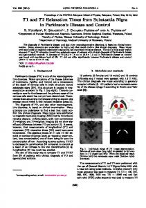
We generated a synthetic phantom to quantitatively evaluate the results of T1 and T2 estimations. The phantom was made of three types of tissues organized in concentric spheres, which are cerebrospinal fluid (CSF), white matter (WM), and gray matter (GM). All reference values are taken as similar to values in the human brain1 (Tab. 1). To demonstrate the capability to retrieve realistic B1 maps, B1 was set to different values: smaller than 1 for GM and higher than 1 for CSF and WM. Since B1 is generally high at the center of the scene [5], we set B1 for CSF to be the largest among all tissues. The reference value of k is set to be 7. The reference relaxation maps (see Fig. 1) were used to feed 1

The T1 , T2 and M0 values are given by http://www.bic.mni.mcgill.ca/brainweb/

19

MICCAI Workshop - IntellMR 2014

Simultaneous T1 , T2 and B1 Mapping

5

Fig. 1. The synthetic phantom. From left to right: B1 , T1 , T2 and M0 reference maps.

into an MRI simulator2 in order to synthesize T1 and T2 relaxometry sequences following signal equations from Sect. 2.1 with α accounting for B1 . Then we added Rician noise to the simulated relaxometry sequences (SNR= 20dB). The estimation was run with the regular DESPOT1 and EPG estimations (Sect. 2.1) and with the proposed method. The results were then compared to the reference values to quantitatively evaluate our algorithm. 3.2

In Vivo Study

In vivo validation was performed on a high field MRI scanner (3T Siemens Verio VB17), which has significant effects of B1 field inhomogeneities. Wholebrain MR images were acquired on 13 healthy subjects (6 male, 7 female, mean age= 29.2 ± 17.8 y.o.). To compensate for between-scans subject motion, a sixparameter rigid-body registration was carried out for each subject based on normalized mutual information. We acquired T1-w SE and T2-w/PD-w MR sequences for each subject and considered these real acquisitions as references for in vivo validation. Then the estimated maps (with our method and with the methods described in Sect. 2.1) were used to feed into the MRI simulator2 to generate T1-w, T2-w and PD-w images with the same sequences and parameters as the real acquisitions. Note that for all simulations, we applied bias field correction of the M0 map as it is sensitive to the coil sensitivity. This correction is based on a unified segmentation [1]. To quantitatively evaluate the performance of the algorithms, we use the squared correlation coefficient R, computed between the real and the simulated images, as an indicator of the estimation accuracy. Assuming the simulations are perfect, the closer the R values are to 1, the better the map estimations.

4

Results

4.1

Synthetic Phantom

We present in Tab. 1 the comparison between the reference and estimated values for T1 , T2 , B1 and M0 using the two evaluated methods. It can be seen that the DESPOT1 algorithm is sensitive to B1 inhomogeneities due to its inability to 2

SimuBloch v0.3 at http://vip.creatis.insa-lyon.fr

20

MICCAI Workshop - IntellMR 2014

6

F. Cao et. al.

estimate those values. The estimated T1 and M0 therefore vary significantly from the reference values. However, when we applied the proposed algorithm, the estimated B1 , T1 , T2 and M0 are in close agreement with the reference values. The reference values are always included within one standard deviation of the estimated values using the proposed method.

Tissue Method Ave(B1 ) Std(B1 ) 0.00 Reference 1.10 – WM Regular – Proposed 1.10 0.00 0.00 Reference 0.80 – GM Regular – Proposed 0.80 0.00 0.00 Reference 1.30 – CSF Regular – Proposed 1.30 0.00

Ave(T1 ) Std(T1 ) 0.00 500.00 0.71 608.06 495.97 15.71 0.00 830.00 0.87 526.88 823.50 60.30 0.00 2500.00 4364.33 449.69 2485.96 193.76

Ave(T2 ) Std(T2 ) Ave(M0 ) Std(M0 ) 0.00 0.00 70.00 80.00 1.97 1.59 71.31 77.55 69.84 1.69 80.32 1.13 0.00 0.00 80.00 90.00 2.47 1.47 87.26 79.10 79.91 2.57 90.22 3.12 0.00 100.00 0.00 330.00 1.12 476.14 48.61 75.95 329.73 27.13 100.50 3.33

Table 1. Statistical values of B1 , T1 (ms), T2 (ms) and M0 on the synthetic phantom. Ave and Std are the mean and standard deviation. The estimated k is 6.94.

4.2

In Vivo Results

Fig. 2 presents the maps estimated using the regular method and the proposed algorithm. This figure confirms visually that the regular algorithm is sensitive to B1 inhomogeneities, especially seen on T1 maps where the center values are much higher for the same tissues. On the contrary, the proposed method removes the influence of B1 inhomogeneities and the obtained maps are much more uniform. Fig. 3 presents the T1-w images from the real acquisition and from the simulation using the regular method and the proposed algorithm. The results of T2-w and PD-w simulations were computed for quantitative evaluation but are not presented as all simulations look very similar to the real acquisitions. On this figure, it is clear that the regular method’s inability to estimate B1 results in degraded simulations for T1-w sequences. These observations are confirmed by the R coefficients in Tab. 2. All values are significantly increased (paired t-test, p < 10−6 for each of the simulated sequences) between the regular and proposed methods. Moreover, the correlation coefficients for T1-w images increase over 50% using the proposed method (0.653 compared to 0.327).

5

Conclusion

We have proposed a new approach for simultaneous mapping of B1 inhomogeneity field, T1 and T2 relaxation times, and proton density M0 . The method is based on the intrinsic correlation between the T1 and T2 relaxometry sequences. We use a combined model of DESPOT1 and EPG algorithms to estimate T1 , T2 , M0 and

21

MICCAI Workshop - IntellMR 2014

Simultaneous T1 , T2 and B1 Mapping

(a) No B1 map

(b) T1

(c) T2

(d) M0

(e) B1

(f) T1

(g) T2

(h) M0

7

Fig. 2. Estimated maps on one healthy subject. Row 1 shows the maps using the regular method, row 2 using the proposed method. From left to right for each row: B1 , T1 , T2 and M0 maps respectively. The same window level is set for each column.

Fig. 3. Simulated T1-w images and the corresponding real acquisition on one healthy subject. From left to right: real acquisition, simulated images using the regular and the proposed methods respectively.

Regular Proposed

T1-w Ave(R) T1-w Std(R) T2-w Ave(R) T2-w Std(R) PD-w Ave(R) PD-w Std(R) 0.327 0.092 0.894 0.018 0.729 0.051 0.653 0.107 0.923 0.016 0.834 0.026

Table 2. Average correlation coefficient R between the simulated images and the real acquisitions on 13 healthy subjects, for T1-w, T2-w and PD-w images. Row 1 shows R for the regular method, row 2 for the proposed algorithm. Differences are significant (paired t-test, p < 10−6 ).

B1 simultaneously. This combination requires no additional sequence for the B1 correction, making use of the traditional T1 and T2 relaxometry sequences only.

22

MICCAI Workshop - IntellMR 2014

8

F. Cao et. al.

Our experiments on simulated data demonstrated that the proposed method is able to accurately estimate T1 , T2 , M0 and B1 maps. Experiments on in vivo data showed high correlation (up to 50 % increase) between the weighted acquisitions and the simulated sequences, which confirms the great potential of the proposed method to handle clinical applications where quantitative MRI has been shown to be highly relevant (MS, stroke, pediatrics, ...).

References 1. Ashburner, J., Friston, K.: Unified segmentation. NeuroImage 26, 839–851 (2005) 2. Collins, C.M., Li, S., Smith, M.B.: SAR and B1 field distributions in a heterogeneous human head model within a birdcage coil. MRM 40(6), 847–56 (1998) 3. Deoni, S.: High-resolution T1 mapping of the brain at 3T with driven equilibrium single pulse observation of T1 with high-speed incorporation of RF field inhomogeneities (DESPOT1-HIFI). J Magn Reson Imaging 26(4), 1106–11 (2007) 4. Deoni, S., Rutt, B., Peters, T.: Rapid combined T1 and T2 mapping using gradient recalled acquisition in the steady state. MRM 49(3), 515–526 (2003) 5. Dowell, N.G., Tofts, P.S.: Fast, accurate, and precise mapping of the RF field in vivo using the 180 degrees signal null. Magn Reson Med 58(3), 622–30 (2007) 6. Gelman, N., Gorell, J., Barker, P., Savage, R., Spickler, E., Windham, J., Knight, R.: MR imaging of human brain at 3T: preliminary report on transverse relaxation rates and relation to estimated iron content. Radiology 210(3), 759–767 (1999) 7. Hennig, J.: Multiecho imaging sequences with low refocusing flip angles. Journal of Magnetic Resonance (1969) 78(3), 397–407 (Jul 1988) 8. Layton, K., Morelande, M., Wright, D., Farrell, P., Moran, B., Johnston, L.: Modelling and estimation of multicomponent T2 distributions. IEEE TMI 32(8), 1423– 1434 (2013) 9. Lebel, R.M., Wilman, A.H.: Transverse relaxometry with stimulated echo compensation. Magn. Reson. Med. 64(4), 1005–1014 (2010) 10. Parker, G.J.M., Barker, G.J., Tofts, P.S.: Accurate multislice gradient echo T1 measurement in the presence of non-ideal RF pulse shape and RF field nonuniformity. Magnetic Resonance in Medicine 45(5), 838–845 (2001) 11. Powell, M.: The BOBYQA algorithm for bound constrained optimization without derivatives. Tech. rep., Centre for Mathematical Sciences, University of Cambridge, UK (2009) 12. Prasloski, T., Mädler, B., Xiang, Q.S.S., MacKay, A., Jones, C.: Applications of stimulated echo correction to multicomponent T2 analysis. Magnetic resonance in medicine 67(6), 1803–1814 (Jun 2012) 13. Stanisz, G., Odrobina, E., Pun, J., Escaravage, M., Graham, S., Bronskill, M., Henkelman, R.: T1, T2 relaxation and magnetization transfer in tissue at 3T. MRM 54(3), 507–512 (2005) 14. Tofts, P.: Quantitative MRI of the Brain: Measuring Changes Caused by Disease. John Wiley & Sons, Ltd (2003) 15. Treier, R., Steingoetter, A., Fried, M., Schwizer, W., Boesiger, P.: Optimized and combined T1 and B1 mapping technique for fast and accurate T1 quantification in contrast-enhanced abdominal MRI. Magn Reson Med 57(3), 568–76 (2007) 16. Tukey, J.: Exploratory Data Analysis. Addison-Wesley Publishers, Cy (1977) 17. Yarnykh, V.L.: Actual flip-angle imaging in the pulsed steady state: A method for rapid three-dimensional mapping of the transmitted radiofrequency field. Magn. Reson. Med. 57(1), 192–200 (Jan 2007)

23