gory might be annotated with âtree,â âflower,â and âsky.â .... predicted annotations: athlete, sky, tree, water ..... image classification on the UIUCâSport dataset.
Simultaneous Image Classification and Annotation Chong Wang, David Blei, Li Fei-Fei Computer Science Department Princeton University {chongw, blei, feifeili}@cs.princeton.edu
Abstract
an office scene is unlikely to be annotated with “swimming pool” or “sunbather.” In this paper, we develop a probabilistic model that simultaneously learns the salient patterns among images that are predictive of their class labels and annotation terms. For new unknown images, our model provides predictive distributions of both class and annotation. We build on recent machine learning and computer vision research in probabilistic topic models, such as latent Dirichlet allocation (LDA) [4] and probabilistic latent semantic indexing [10] (pLSI). Probabilistic topic models find a low dimensional representation of data under the assumption that each data point can exhibit multiple components or “topics.” While topic models were originally developed for text, they have been successfully adapted and extended to many computer vision problems [2, 1, 8, 9, 23, 5]. Our model finds a set of image topics that are predictive of both class label and annotations. The two main contributions of this work are:
Image classification and annotation are important problems in computer vision, but rarely considered together. Intuitively, annotations provide evidence for the class label, and the class label provides evidence for annotations. For example, an image of class highway is more likely annotated with words “road,” “car,” and “traffic” than words “fish,” “boat,” and “scuba.” In this paper, we develop a new probabilistic model for jointly modeling the image, its class label, and its annotations. Our model treats the class label as a global description of the image, and treats annotation terms as local descriptions of parts of the image. Its underlying probabilistic assumptions naturally integrate these two sources of information. We derive an approximate inference and estimation algorithms based on variational methods, as well as efficient approximations for classifying and annotating new images. We examine the performance of our model on two real-world image data sets, illustrating that a single model provides competitive annotation performance, and superior classification performance.
1. We extended supervised topic modeling [3] (sLDA) to classification problems. SLDA was originally developed for predicting continuous response values, via a linear regression. We note that the multi-class extension presented here is not simply a “plug-and-play” extension of [3]. As we show in Section 2.2, it requires substantial development of the underlying inference and estimation algorithms.
1. Introduction Developing automatic methods for managing large volumes of digital information is increasingly important as online resources continue to be a vital resource in everyday life. Among these methods, automatically organizing and indexing multimedia data remains an important challenge. We consider this problem for image data that are both labeled with a category and annotated with free text. In such data, the class label tends to globally describe each image, while the annotation terms tend to describe its individual components. For example, an image in the outdoor category might be annotated with “tree,” “flower,” and “sky.” Image classification and image annotation are typically treated as two independent problems. Our motivating intuition, however, is that these two tasks should be connected. An image annotated with “car” and “pedestrian” is unlikely to be labeled as a living room scene. An image labeled as
2. We embed a probabilistic model of image annotation into the resulting supervised topic model. This yields a single coherent model of images, class labels and annotation terms, allowing classification and annotation to be performed using the same latent topic space. We find that a single model, fit to images with class labels and annotation terms, provides state-of-the-art annotation performance and exceeds the state-of-the-art in classification performance. This shows that image classification and annotation can be performed simultaneously. This paper is organized as follows. In Section 2, we describe our model and derive variational algorithms for inference, estimation, and prediction. In Section 3, we describe 1
related work. In Section 4, we study the performance of our models on classification and annotation for two real-world image datasets. We summarize our findings in Section 5.
2. Models and Algorithms In this section, we develop two models: multi-class sLDA and multi-class sLDA with annotations. We derive a variational inference algorithm for approximating the posterior distribution, and an approximate parameter estimation algorithm for finding maximum likelihood estimates of the model parameters. Finally, we derive prediction algorithms for using these models to label and annotate new images.
2.1. Modeling images, labels and annotations The idea behind our model is that class and annotation are related, and we can leverage that relationship by finding a latent space predictive of both. Our training data are images that are categorized and annotated. In testing, our goal is to predict the category and annotations of a new image. Each image is represented as a bag of “codewords” r1:N , which are obtained by running the k-means algorithm on patches of the images [15, 18]. (See Section 4 for more details about our image features.) The category c is a discrete class label. The annotation w1:M is a collection of words from a fixed vocabulary. We fix the number of topics K and let C denote the number of class labels. The parameters of our model are a set of K image topics π1:K , a set of K annotation topics β1:K , and a set of C class coefficients η1:C . Each coefficient ηc is a K-vector of real values. Each “topic” is a distribution over a vocabulary, either image codewords or annotation terms. Our model assumes the following generative process of an image, its class label, and its annotation. 1. Draw topic proportions θ ∼ Dir(α). 2. For each image region rn , n ∈ {1, 2, . . . , N }: (a) Draw topic assignment zn | θ ∼ Mult(θ). (b) Draw region codeword rn | zn ∼ Mult(πzn ). 3. Draw class label c | z1:N ∼ softmax(¯ z , η), where z¯ = PN 1 z is the empirical topic frequencies and the n=1 n N softmax function provides the following distribution, � PC � p(c | z¯, η) = exp ηcT z¯ / l=1 exp ηl⊤ z¯ . 4. For each annotation term wm , m ∈ {1, 2, . . . , M }:
(a) Draw region identifier ym ∼ Unif{1, 2, . . . , N } (b) Draw annotation term wm ∼ Mult(βzn ). Figure 1(a) illustrates our model as a graphical model. We refer to this model as multi-class sLDA with annotations. It models both the image class and image annotation with the same latent space.
Consider step 3 of the generative process. In modeling the class label, we use a similar set-up as supervised LDA (sLDA) [3]. In sLDA, a response variable for each “document” (here, an image) is assumed drawn from a generalized linear model with input given by the empirical distribution of topics that generated the image patches. In [3], that response variable is real valued and drawn from a linear regression, which simplified inference and estimation. However, a continuous response is not appropriate for our goal of building a classifier. Rather, we consider a class label response variable, drawn from a softmax regression for classification. This complicates the approximate inference and parameter estimation algorithms (see Section 2.2 and 2.3), but provides an important extension to the sLDA framework. We refer to this multi-class extension of sLDA (without the annotation portion) as multi-class sLDA. We note that multi-class sLDA can be used in classification problems outside of computer vision. We now turn to step 4 of the generative process. To model annotations, we use the same generative process as correspondence LDA (corr-LDA) [2], where each annotation word is assumed to be drawn from one of the topics that is associated with an image patch. For example, this will encourage words like “blue” and “white” to be associated with the image topics that describe patches of sky. We emphasize that Corr-LDA and sLDA were developed for different purposes. Corr-LDA finds topics predictive of annotation words; sLDA finds topics predictive of a global response variable. However, both approaches employ similar statistical assumptions. First, generate the image from a topic model. Then, generate its annotation or class label from a model conditioned on the topics which generated the image. Our model uses the same latent topic space to generate both the annotation and class label.
2.2. Approximate inference In posterior inference, we compute the conditional distribution of the latent structure given a model and a labeled annotated image. As for LDA, computing this posterior exactly is not possible [4]. We employ mean-field variational methods for a scalable approximation algorithm. Variational methods consider a simple family of distributions over the latent variables, indexed by free variational parameters, and try to find the setting of those parameters that minimizes the Kullback-Leibler (KL) divergence to the true posterior [13]. In our model, the latent variables are the per-image topic proportions θ, the per-codeword topic assignment zn , and the per-annotation word region identifier ym . Note that there are no latent variables explicitly associated with the class; its distribution is wholly governed by the per-codeword topic assignments.
class: snowboarding annotations: skier, ski, tree, water, boat, building, sky, residential area
predicted class: snowboarding predicted annotations: athlete, sky, tree, water, plant, ski, skier (a)
(b)
Figure 1. (a). A graphical model representation of our model. Nodes represent random variables; edges denote possible dependence between random variables; plates denote replicated structure. Note that in this model, the image class c and image annotation wm are dependent on the topics that generated the image codewords rn . (b). An example image with the class label and annotations from the UIUC-Sport dataset [17]. The italic words are the predicted class label and annotations, using our model.
The mean-field variational distribution is, QN QM q(θ, z, y) = q(θ|γ) n=1 q(zn |φn ) m=1 q(ym |λm ), (1) where φn is a variational multinomial over the K topics, γ is a variational Dirichlet, and λm is a variational multinomial over the image regions. We fit these parameters with coordinate ascent to minimize the KL divergence between q and the true posterior. (This will find a local minimum.) Let Θ = {α, β1:K , η1:C , π1:K }. Following Jordan et al. [14], we bound the log-likelihood of a image-classannotation triple, (r, c, w). We have: log p(r, c, w|Θ) Z p(θ, z, y, r, c, w|Θ)q(θ, z, y) dθdzdy = log q(θ, z, y) ≥Eq [log p(θ, z, y, r, c, w|Θ)] − Eq [q(θ, z, y)] =L(γ, φ, λ; Θ).
(2)
We next turn to the update for the variational multinomial φ. Here, the variational method derived in [3] cannot be used because the expectation of the log partition function for softmax regression (i.e., multi-class classification) cannot be exactly computed. The terms in L containing φn are: L[φn ] =
i=1
log
≥ − log
C X
!#
exp(ηlT z¯)
l=1
C X l=1
! � � T Eq exp(ηl z¯)
� � K X 1 φnj exp ηlj . N n=1 j=1
N C Y X l=1
tion of φn , thus can be written as hT φn , where h = [h1 , · · · , hi , · · · , hK ]T and does not contain φn . For convenience, define bi as follows,
M K X X λmn log βi,wm . γj ) + log πi,rn + bi = Ψ(γi ) − Ψ(
1 T ηc φn − N m=1 " !# K C X X T φni log φni . exp(ηl z¯) − Eq log λmn log βi,wm
l=1
L′[φn ] =
+
i=1
m=1
Now, the lower bound L′[φn ] can be written as
j=1
!
(6)
Plugging Equation 6 into Equation 5, we obtain a lower bound of L[φn ] , which we will denote L′[φn ] . We present a fixed-point iteration for maximizing this proxy. The idea is that given an old estimation of ′ φold n , a lower bound of L[φn ] is constructed so that this lower bound is tight on φold [19]. Then maxin mizing this lower bound of L′[φn ] is solved in closedform and φold We note that n is updated correspondingly. �� PC QN �PK 1 is only a linear funcj=1 φnj exp N ηlj n=1 l=1
j=1
K X γj ) + log πi,rn + φni Ψ(γi ) − Ψ(
M X
Eq
"
= − log
The coordinate ascent updates for γ and λ are the same as those in [2], which uses the same notation: PN γ = α + n=1 φn (3) �P � K λmn ∝ exp (4) i=1 φni log βi,wm .
K X
The hcentral is that exactly computing �P issue here �i C T −Eq log ¯) takes O(K N ) time. To l=1 exp(ηl z address this, we lower bound this term with Jensen’s inequality. This gives:
K X i=1
(5)
φni bi +
K X 1 T φni log φni . ηc φn −log(hT φn )− N i=1
Finally, suppose we have a previous value φold n . For log(x), we know log(x) ≤ ζ −1 x + log(ζ) − 1, ∀x > 0, ζ > 0, where the equality holds if and only if x = ζ. Set
x = hT φn and ζ = hT φold n . Immediately, we have: L′[φn ] ≥
K X
φni bi +
i=1
− log(h
T
φold n )
Next, let Vw denote the number of total annotations, and the terms containing β1:K (with Lagrangian multipliers) are:
1 T −1 T η φn − (hT φold h φn n ) N c +1−
K X
L[β1:K ] (D) =
φni log φni .
(7)
i=1
L′[φn ]
φold n .
This lower bound of is tight when φn = MaxiPK mizing Equation 7 under the constraint i=1 φni = 1 leads to the fixed point update, � PM φni ∝πi,rn exp Ψ(γi ) + m=1 λmn log βi,wm � 1 T old −1 + ηci − (h φn ) hi . (8) N Observe how the per-feature variational distribution over topics φ depends on both class label c and annotation information wm . The combination of these two sources of data has naturally led to an inference algorithm that uses both. The full variational inference procedure repeats the updates of Equations 3, 4 and 8 until Equation 2, the lower bound on the log marginal probability log p(r, c, w|Θ), converges.
2.3. Parameter estimation Given a corpus of image data with class labels and annotations, D = {(rd , wd , cd )}D d=1 , we find the maximum likelihood estimation for image topics π1:K , text topics β1:K and class coefficients η1:C . We use variational EM, which replaces the E-step of expectation-maximization with variational inference to find an approximate posterior for each data point. In the M-step, as in exact EM, we find approximate maximum likelihood estimates of the parameters using expected sufficient statistics computed from the E-step. Recall Θ = {α, β1:K , η1:C , π1:K }. The corpus loglikelihood is, L(D) =
D X
log p(rd , cd , wd |Θ).
(9)
d=1
(We do not optimize α in this paper.) Again, we maximize the lower bound of L(D) by plugging Equations 2 and 6 into Equation 9. Let Vr denote the number of codewords, the terms containing π1:K (with Lagrangian multipliers) are: L[π1:K ] (D) = Nd X K D X X
φdni log πi,rn +
d=1 n=1 i=1
K X i=1
µi
Vr X
f =1
Setting ∂L[π1:K ] (D)/∂πif = 0 leads to πif ∝
Nd D X X
d=1 n=1
1[rn = f ]φdni .
πif − 1 . (10)
K N X M X X
λmn φni log βi,wm +
m=1 n=1 i=1
K X
νi
i=1
Vw X
!
βiw − 1 .
w=1
Setting ∂L[β1:K ] (D)/∂βiw = 0 leads to
βiw ∝
D X M X
1[wm = w]
d=1 m=1
X
φdni λdmn .
(11)
n
Finally, terms containing η1:C are: L[η1:C ] (D) = D X d=1
ηcTd φ¯d
− log
Nd C Y X
c=1 n=1
K X
φdni exp
i=1
�
1 ηci Nd
�!!!
Setting ∂L[η1:C ] (D)/∂ηci = 0 does not lead to a closedform solution. We optimize with conjugate � gradient �� [20]. PC QNd �PK 1 Let κd = c=1 n=1 . Conjui=1 φdni exp Nd ηci gate gradient only requires the derivatives: D � ∂L[η1:C ] (D) X = 1[cd = c]φ¯di − ∂ηci d=1 � � N K D d X X Y 1 κ−1 φdnj exp ηcj × d N d n=1 j=1 d=1 � � 1 1 Nd X Nd φdni exp Nd ηci � � . PK 1 φ exp η n=1 j=1 dnj Nd cj
(12)
2.4. Classification and annotation With inference and parameter estimation algorithms in place, it remains to describe how to perform prediction, i.e. predicting both a class label and annotations from an unknown image. The first step is to perform variational inference given the unknown image. We can use a variant of the algorithm in Section 2.2 to determine q(θ, z). Since the class label and annotations are not observed, we remove the λmn terms from the variational distribution (Equation 1) and the terms involving ηc from the updates on the topic multinomials (Equation 8). In classification, we estimate the probability of the label c by replacing the true posterior p(z|w, r) with the varia-
.
performance of our model to corr-LDA [2]. (Corr-LDA was shown to provide better performance than the previous LDA-based annotation models in [1] and [8].)
tional approximation p(c|r, w) !! Z C X T T ≈ exp ηc z¯ − log exp(ηl z¯) q(z)dz
4. Empirical results
l=1
"
!#!
L X � � ≥ exp Eq ηcT z¯ − Eq log exp(ηlT z¯) l=1
,
where the last equation comes from Jensen’s inequality, and q is the variational posterior computed in the first step. The second term in the exponent is constant with respect to class label. Thus, the prediction rule is � � ¯ (13) c∗ = arg max Eq ηcT z¯ = arg max ηcT φ. c∈{1,...,C}
c∈{1,...,C}
There are two approximations at play. First, we approximate the posterior with q. Second, we approximate the expectation of an exponential using Jensen’s inequality. While there are no theoretical guarantees here, we evaluate this classification procedure empirically in Section 4. The procedure for predicting annotations is the same as in [2]. To obtain a distribution over annotation terms, we average the contributions from each region, p(w|r, c) ≈
N X X
p(w|zn , β)q(zn ).
(14)
n=1 zn
3. Related Work Image classification and annotation are both important problems in computer vision and machine learning. Much previous work has explored the use of global image features for scene (or event) classification [21, 27, 26, 28, 17], and both discriminative and generative techniques have been applied to this problem. Discriminative methods include the work in [7, 30, 29, 16]. Generative methods include the work in [9, 6, 22, 17]. In the work of [5], the authors combine generative models for latent topic discovery [11] and discriminative methods for classification (knearest neighbors). LDA-based image classification was introduced in [9], where each category is identified with its own Dirichlet prior, and that prior is optimized to distinguish between them. The multi-class sLDA model combines the generative and discriminative approaches, which may be better for modeling categorized images (see Section 4). For image annotation, several studies have explored the use of probabilistic models to learn the relationships between images and annotation terms [1, 8, 12]. Our model is most related to the family of models based on LDA, which were introduced to image annotation in [8]. But the idea that image annotation and classification might share the same latent space has not been studied. We will compare the
We test our models with two real-world data sets that contain class labels and annotations: a subset from LabelMe [24] and the UIUC-Sport data from [17]. In the LabelMe data, we used the on-line tool to obtain images from the following 8 classes: “highway,” “inside city,” “tall building,” “street,” “forest,” “coast,” “mountain,” and “open country.” We first only kept the images that were 256 × 256 pixels, and then randomly selected 200 images for each class. (In doing this, we attempted to obtain the same image data as described in [9].) The total number of images is 1600. The UIUC-Sport dataset [17] contains 8 types of sports: “badminton,” “bocce,” “croquet,” “polo,” “rockclimbing,” “rowing,” “sailing” and “snowboarding.” The number of images in each class varies from 137 (bocce) to 250 (rowing). The total number of images is 1792. Following the setting in [9], we use the 128-dimensional SIFT [18] region descriptors selected by a sliding grid (5 × 5). We ran the k-means algorithm [15] to obtain the codewords and codebook. We report on a codebook of 240 codewords. (Other codebook sizes gave similar performance.) In both data sets, we removed annotation terms that occurred less than 3 times. On average, there are 6 terms per annotation in the LabelMe data, and 8 terms per annotation in the UIUC-Sport data. Finally, We evenly split each class to create the training and testing sets. Our procedure is to train the multi-class sLDA with annotations on labeled and annotated images, and train the multi-class sLDA model on labeled images. All testing is on unlabeled and unannotated images. See Figure 4 for example annotations and classifications from the multi-class sLDA with annotations. Image Classification. To assess our models on image classification, we compared the following methods, 1. Fei-Fei and Perona, 2005: This is the model from [9]. It is trained on labeled images without annotation. 2. Bosch et al., 2006: This is the model described in [5]. It first employs pLSA [11] to learn latent topics, and then uses the k-nearest neighbor (KNN) classifier for classification. We use unsupervised LDA1 to learn the latent topics and, following [5], set the number of neighbors to be 10. As for the other models considered here, we use SIFT features. We note that [5] use other types of features as well. 1 According to [25], pLSA performs similarly to unsupervised LDA in practice.
image classification on the LabelMe dataset
image classification on the UIUC−Sport dataset
0.78 0.66 0.76
0.64 average accuracy
average accuracy
0.74 0.72 0.7 0.68 0.66
0.62
0.6
0.58
0.64 0.56 20
40
60
80
100
multi−class sLDA with annotations
120
topics
20
multi−class sLDA
40
60
Fei−Fei and Perona, 2005
80
100
120
topics
Bosch et al., 2006
Figure 2. Comparisons of average accuracy over all classes based on 5 random train/test subsets. multi-class sLDA with annotations and multi-class sLDA (red curves in color) are both our models. left. Accuracy as a function of the number of topics on the LabelMe dataset. right. Accuracy as a function of the number of topics on the UIUC-Sport dataset.
3. multi-class sLDA: This is the multi-class sLDA model, described in this paper. 4. multi-class sLDA with annotations: This is multi-class sLDA with annotations, described in this paper. Note all testing is performed on unlabeled and unannotated images. The results are illustrated in the graphs of Figure 2 and in the confusion matrices of Figure 3.2 Our models—multiclass sLDA and multi-class sLDA with annotations— perform better than the other approaches. They reduce the error of Fei-Fei and Perona, 2005 by at least 10% on both data sets, and even more for Bosch et al., 2006. This demonstrates that multi-class sLDA is a better classifier, and that joint modeling does not negatively affect classification accuracy when annotation information is available. In fact, it usually increases the accuracy. Observe that the model of [5], unsupervised LDA combined with KNN, gives the worst performance of these methods. This highlights the difference between finding topics that are predictive, as our models do, and finding topics in an unsupervised way. The accuracy of unsupervised LDA might be increased by using some of the other visual features suggested by [5]. Here, we restrict ourselves to SIFT features in order to compare models, rather than feature sets. As the number of topics increases, the multi-class sLDA models (with and without annotation) do not overfit until around 100 topics, while Fei-Fei and Perona, 2005 begins to overfit at 40 topics. This suggests that multi-class sLDA, which combines aspects of both generative and discriminative classification, can handle more latent features than a purely generative approach. On one hand, a large number 2 Other
than the topic models listed, we also tested an SVM-based approach using SIFT image features. The SVM yielded much worse performance than the topic models (47% for the LabelMe data, and 20% for the UIUC-Sport data). These are not marked on the plots.
of topics increases the possibility of overfitting; on the other hand, it provides more latent features for building the classifier.
Image Annotation. In the case of multi-class sLDA with annotations, we can use the same trained model for image annotation. We emphasize that our models are designed for simultaneous classification and annotation. For image annotation, we compare following two methods, 1. Blei and Jordan, 2003: This is the corr-LDA model from [2], trained on annotated images. 2. multi-class sLDA with annotations: This is exactly the same model trained for image classification in the previous section. In testing annotation, we observe only images. To measure image annotation performance, we use an evaluation measure from information retrieval. Specifically, we examine the top-N F-measure3 , denoted as Fmeasure@N , where we set N = 5. We find that multiclass sLDA with annotations performs slightly better than corr-LDA over all the numbers of topics tested (about 1% relative improvement). For example, considering models with 100 topics, the LabelMe F-measures are 38.2% (corrLDA) and 38.7% (multi-class sLDA with annotations); on UIUC-Sport, they are 34.7% (corr-LDA) and 35.0% (multiclass sLDA with annotations). These results demonstrate that our models can perform classification and annotation with the same latent space. With a single trained model, we find the annotation performance that is competitive with the state-of-the-art, and classification performance that is superior. 3 F-measure
is defined as 2 ∗ precision ∗ recall/(precision + recall).
multi−class sLDA with annotations
multi−class sLDA
.77 .01 .01 .05 .00 .05 .03 .08
highw.
insid.
.02 .73 .05 .18 .01 .00 .01 .00
insid.
tallb.
.00 .06 .85 .05 .01 .00 .02 .01
tallb.
street
.05 .16 .04 .72 .00 .00 .01 .02
street
forest
.00 .00 .00 .00 .92 .00 .04 .04
highw.
.77 .02 .01 .04 .00 .05 .04 .07
multi−class sLDA with annotations badmi.
.81 .04 .08 .02 .00 .01 .02 .02
.01 .75 .04 .17 .00 .01 .00 .02
bocce
.01 .06 .84 .04 .01 .00 .03 .01
croquet
.05 .17 .04 .71 .00 .00 .01 .02
forest
multi−class sLDA badmi.
.82 .02 .09 .03 .00 .01 .02 .01
.09 .31 .36 .05 .03 .04 .02 .11
bocce
.07 .26 .43 .05 .04 .03 .03 .08
.02 .08 .70 .08 .02 .04 .04 .02
croquet
.02 .08 .70 .08 .02 .04 .04 .02
polo
.10 .03 .19 .53 .01 .08 .02 .04
polo
.10 .03 .22 .51 .01 .06 .02 .05
.00 .00 .00 .00 .92 .00 .04 .04
rockc
.00 .02 .01 .03 .83 .01 .01 .09
rockc
.00 .02 .01 .03 .85 .01 .01 .07 .03 .02 .10 .07 .01 .71 .03 .03
coast
.12 .01 .00 .00 .01 .69 .01 .16
coast
.10 .00 .00 .00 .01 .71 .01 .17
rowing
.03 .02 .08 .07 .01 .73 .04 .03
rowing
mount.
.03 .00 .01 .01 .03 .00 .82 .10
mount.
.03 .00 .01 .01 .02 .00 .83 .10
sailing
.03 .01 .09 .03 .01 .07 .69 .07
sailing
.03 .00 .11 .03 .01 .07 .66 .09
openc.
.06 .00 .00 .01 .08 .11 .11 .62
openc.
.07 .00 .01 .01 .08 .12 .10 .61
snowb.
.03 .05 .07 .03 .08 .06 .04 .64
snowb.
.02 .05 .07 .05 .12 .04 .05 .60
o m c fo s ta in hw sid. llb. tree res oast oun pen t t c. t. .
hig
(a) LabelMe: avg. accuracy: 76%
o m c fo s ta in hw sid. llb. tree res oast oun pen t t c. t. .
hig
s s r r p c b dm occ roqu olo ockc owin ailin now e g b. g et i.
ba
s s r r p c b dm occ roqu olo ockc owin ailin now e g b. g et i.
ba
(b) LabelMe: avg. accuracy: 76% (c) UIUC-Sport: avg. accuracy: 66% (d) UIUC-Sport: avg. accuracy: 65%
Figure 3. Comparisons using confusion matrices, all from the 100-topic models using multi-class sLDA with annotations and multi-class sLDA. (a) multi-class sLDA with annotations on the LabelMe dataset. (b) multi-class LDA on the LabelMe dataset. (c) multi-class sLDA with annotations on the UIUC-Sport dataset. (d) multi-class sLDA model on the UIUC-Sport dataset.
5. Discussion We have developed a new graphical model for learning the salient patterns in images that are simultaneously predictive of class and annotations. In the process, we have derived the multi-class setting of supervised topic models and studied its performance for computer vision problems. On real-world image data, we have demonstrated that the proposed model is on par with state-of-the-art image annotation methods and outperforms current state-of-the-art image classification methods. Guided by the intuition that classification and annotation are related, we have illustrated that the same latent space can be used to predict both. Acknowledgments. David M. Blei is supported by ONR 175-6343, NSF CAREER 0745520, and grants from Google and Microsoft. Li Fei-Fei is supported by a Microsoft Research New Faculty Fellowship and a grant from Google.
References [1] K. Barnard, P. Duygulu, N. de Freitas, D. Forsyth, D. Blei, and M. Jordan. Matching words and pictures. JMLR, 3:1107–1135, 2003. [2] D. M. Blei and M. I. Jordan. Modeling annotated data. In SIGIR, 2003. [3] D. M. Blei and J. D. McAuliffe. Supervised topic models. In NIPS, 2007. [4] D. M. Blei, A. Ng, and M. I. Jordan. Latent Dirichlet allocation. JMLR, 3:993–1002, 2003. [5] A. Bosch, A. Zisserman, and X. Munoz. Scene classification via pLSA. In ECCV, 2006. [6] L. Cao and L. Fei-Fei. Spatially coherent latent topic model for concurrent object segmentation and classification. In CVPR, 2007. [7] Y. Chen and J. Z. Wang. Image categorization by learning and reasoning with regions. JMLR, 5:913–939, 2004. [8] P. Duygulu, K. Barnard, J. F. G. de Freitas, and D. A. Forsyth. Object recognition as machine translation: Learning a lexicon for a fixed image vocabulary. In ECCV, 2002. [9] L. Fei-Fei and P. Perona. A Bayesian hierarchical model for learning natural scene categories. In CVPR, 2005.
[10] T. Hofmann. Probabilistic latent semantic indexing. In SIGIR, 1999. [11] T. Hofmann. Unsupervised learning by probabilistic latent semantic analysis. Mach. Learn., 42(1-2):177–196, 2001. [12] J. Jeon, V. Lavrenko, and R. Manmatha. Automatic image annotation and retrieval using cross-media relevance models. In SIGIR, 2003. [13] M. I. Jordan, Z. Ghahramani, T. Jaakkola, and L. K. Saul. An introduction to variational methods for graphical models. Machine Learning, 37(2):183–233, 1999. [14] M. I. Jordan, Z. Ghahramani, T. S. Jaakkola, and L. Saul. An introduction to variational methods for graphical models. Learning in Graphical Models, 1999. [15] T. Kadir and M. Brady. Saliency, scale and image description. IJCV, 45(2):83–105, 2001. [16] S. Lazebnik, C. Schmid, and J. Ponce. Beyond bags of features: Spatial pyramid matching for recognizing natural scene categories. In CVPR, 2006. [17] L.-J. Li and L. Fei-Fei. What, where and who? Classifying event by scene and object recognition. In ICCV, 2007. [18] D. Lowe. Object recognition from local scale-invariant features. In ICCV, 1999. [19] T. M. Minka. Estimating a Dirichlet distribution. http://research.microsoft.com/˜minka/papers/dirichlet/, 2000. [20] J. Nocedal and S. J. Wright. Numerical Optimization. Springer, 2006. [21] A. Oliva and A. B. Torralba. Modeling the shape of the scene: A holistic representation of the spatial envelope. IJCV, 42(3):145–175, 2001. [22] P. Quelhas, F. Monay, J.-M. Odobez, D. Gatica-Perez, T. Tuytelaars, and L. J. V. Gool. Modeling scenes with local descriptors and latent aspects. In ICCV, 2005. [23] B. Russell, A. Efros, J. Sivic, W. Freeman, and A. Zisserman. Using multiple segmentations to discover objects and their extent in image collections. In CVPR, 2006. [24] B. C. Russell, A. B. Torralba, K. P. Murphy, and W. T. Freeman. LabelMe: A database and web-based tool for image annotation. IJCV, 77(1-3):157–173, 2008. [25] J. Sivic, B. C. Russell, A. A. Efros, A. Zisserman, and W. T. Freeman. Discovering object categories in image collections. In ICCV, 2005. [26] M. Szummer and R. W. Picard. Indoor-outdoor image classification. In IEEE International Workshop on Content-based Access of Image and Video Databases, 1998.
Correct classification with predicted annotations
highway car, sign, road
inside city buildings, car, sidewalk
tall building trees, buildings occluded, window
street
Incorrect classification (correct class) with predicted annotations
coast (highway) car, sand beach, tree
street (inside city) window, tree, building occluded
inside city (tall building) tree, car, sidewalk
highway (street)
tree, car, sidewalk
car, window, tree
forest
mountain (forest)
tree trunk, trees, ground grass
coast
snowy mountain, tree trunk
open country (coast)
sand beach, cloud
sea water, buildings
mountain
highway (mountain)
snowy mountain, sea water, field
tree, snowy mountain
open country
coast (open country)
cars, field, sand beach
tree, field, sea water
Figure 4. Example results from the LabelMe dataset. For each class, left side contains examples with correct classification and predicted annotations, while right side contains wrong ones (the class label in the bracket is the right one) with the predicted annotations. The italic words indicate the class label, while the normal words are associated predicted annotations. [27] A. Vailaya, M. A. T. Figueiredo, A. K. Jain, and H. Zhang. Image classification for content-based indexing. IEEE Trans. on Image Processing, 10(1):117–130, 2001. [28] J. Vogel and B. Schiele. A semantic typicality measure for natural scene categorization. In DAGM-Symposium, 2004.
[29] Y. Wang and S. Gong. Conditional random field for natural scene categorization. In BMVC, 2007. [30] Z.-H. Zhou and M.-L. Zhang. Multi-instance multi-label learning with application to scene classification. In NIPS, 2006.