IEEE TRANSACTIONS ON SIGNAL PROCESSING, VOL. 62, NO. 5, MARCH 1, 2014
1109
Simultaneous Low-Pass Filtering and Total Variation Denoising Ivan W. Selesnick, Senior Member, IEEE, Harry L. Graber, Member, IEEE, Douglas S. Pfeil, and Randall L. Barbour
Abstract—This paper seeks to combine linear time-invariant (LTI) filtering and sparsity-based denoising in a principled way in order to effectively filter (denoise) a wider class of signals. LTI filtering is most suitable for signals restricted to a known frequency band, while sparsity-based denoising is suitable for signals admitting a sparse representation with respect to a known transform. However, some signals cannot be accurately categorized as either band-limited or sparse. This paper addresses the problem of filtering noisy data for the particular case where the underlying signal comprises a low-frequency component and a sparse or sparse-derivative component. A convex optimization approach is presented and two algorithms derived: one based on majorization-minimization (MM), and the other based on the alternating direction method of multipliers (ADMM). It is shown that a particular choice of discrete-time filter, namely zero-phase noncausal recursive filters for finite-length data formulated in terms of banded matrices, makes the algorithms effective and computationally efficient. The efficiency stems from the use of fast algorithms for solving banded systems of linear equations. The method is illustrated using data from a physiological-measurement technique (i.e., near infrared spectroscopic time series imaging) that in many cases yields data that is well-approximated as the sum of low-frequency, sparse or sparse-derivative, and noise components. Index Terms—Total variation denoising, sparse signal, sparsity, low-pass filter, Butterworth filter, zero-phase filter.
I. INTRODUCTION
L
INEAR TIME-INVARIANT (LTI) filters are widely used in science, engineering, and general time series analysis. The properties of LTI filters are well understood, and many effective methods exist for their design and efficient implementation [62]. Roughly, LTI filters are most suitable when the signal of interest is (approximately) restricted to a known frequency band. At the same time, the effectiveness of an alternate approach to signal filtering, based on sparsity, has been increasingly recognized [22], [34], [60], [74]. Over the past 10–15 years, the development of algorithms and theory for sparsityManuscript received January 03, 2013; revised September 13, 2013 and December 19, 2013; accepted December 20, 2013. Date of publication January 09, 2014; date of current version February 07, 2014. The associate editor coordinating the review of this manuscript and approving it for publication was prof. Jean-Christophe Pesquet. This research was supported by the NSF under Grant No. CCF-1018020, the NIH under Grant Nos. R42NS050007, R44NS049734, and R21NS067278, and by DARPA project N66001-10-C-2008. I. W. Selesnick is with the Department of Electrical and Computer Engineering, NYU Polytechnic School of Engineering, Brooklyn, NY 11201 USA (e-mail:
[email protected]). H. L. Graber, D. S. Pfeil, and R. L. Barbour are with the Department of Pathology, SUNY Downstate Medical Center, Brooklyn, NY 11203 USA. This material includes MATLAB software implementing the algorithms described herein. The material is 0.7 MB in size. Digital Object Identifier 10.1109/TSP.2014.2298836
based signal processing has been an active research area, and many algorithms for sparsity-based denoising (and reconstruction, etc.) have been developed [67], [73]. These are most suitable when the signal of interest either is itself sparse or admits a sparse representation. However, the signals arising in some applications are more complex: they are neither isolated to a specific frequency band nor do they admit a highly sparse representation. For such signals, neither LTI filtering nor sparsity-based denoising is appropriate by itself. Can conventional LTI filtering and more recent sparsity-based denoising methods be combined in a principled way, to effectively filter (denoise) a wider class of signals than either approach can alone? This paper addresses the problem of filtering noisy data where the underlying signal comprises a low-frequency component and a sparse or sparse-derivative component. It is assumed here can be modeled as that the noisy data (1) where is a low-pass signal, is a sparse and/or sparse-derivative signal, and is stationary white Gaussian noise. For noisy data such as in (1), neither conventional low-pass filtering nor sparsity-based denoising is suitable. Further, (1) is a good model for many types of signals that arise in practice, for example, in nano-particle biosensing (e.g., Fig. 3(a) in [30]) and near infrared spectroscopic (NIRS) imaging (e.g., Fig. 9 in [3]). Note that if the low-pass signal were observed in noise , then low-pass filtering (LPF) would proalone . On the other vide a good estimate of ; i.e., hand, if were a sparse-derivative signal observed in noise , then total variation denoising (TVD) would alone [68]. Given provide a good estimate of ; i.e., , we seek a simple optinoisy data of the form mization-based approach that enables the estimation of and individually. In this paper, an optimization approach is presented that enables the simultaneous use of low-pass filtering and sparsitybased denoising to estimate a low-pass signal and a sparse signal from a single noisy additive mixture, cf. (1). The optimization problem we formulate involves the minimization of a non-differentiable, strictly convex cost function. We present two iterative algorithms.1 The first algorithm models in (1) as having a sparse derivative and is derived using the majorization-minimization (MM) principle. The second algorithm models in (1) as having a sparse derivative, or being sparse itself, or both. This algorithm is derived using the alternating direction method of multipliers (ADMM). The second algorithm is more general 1Software
is available at http://eeweb.poly.edu/iselesni/lpftvd/
1053-587X © 2014 IEEE. Personal use is permitted, but republication/redistribution requires IEEE permission. See http://www.ieee.org/publications_standards/publications/rights/index.html for more information.
1110
and can be used in place of the first. However, as will be illustrated below (Section VII-C), in cases where the first algorithm is applicable, it is preferable to the second one, because it converges faster and does not require a step-size parameter as the second algorithm does. In addition, this paper explains how a suitable choice of discrete-time filter makes the proposed approach effective and computationally efficient. Namely, we describe the design and implementation of a zero-phase non-causal recursive filter for finite-length data, formulated in terms of banded matrices. We choose recursive filters for their computational efficiency in comparison with non-recursive filters, and the zero-phase property to eliminate phase distortion (phase/time offset issues). As the algorithms are intended primarily for batch-mode processing, the filters need not be causal. We cast the recursive discrete-time filter in terms of a matrix formulation so as to easily and accurately incorporate it into the optimization framework and because it facilitates the implementation of the filter on finite-length data. Furthermore, the formulation is such that all matrix operations in the devised algorithms involve only banded matrices, thereby exploiting the high computational efficiency of solvers for banded linear systems ([65], Section 2.4) and of sparse matrix multiplication. The computational efficiency of the proposed algorithms also draws on recent developments in sparse-derivative signal denoising (i.e., total variation (TV) denoising [10], [19], [68]). In particular, we note that the exact solution to the 1D TV denoising problem can be calculated by fast constructive algorithms [27], [49]. The algorithms presented here draw on this and the ‘fused lasso signal approximator’ [40]. After Section II on preliminaries, Section III presents the formulation of the optimization problem for simultaneous low-pass filtering and sparse-signal denoising. Section IV derives an iterative algorithm for solving the optimization problem. Section V addresses the case where both the signal itself and its derivative are sparse. Section VI presents recursive discrete-time filters to be used in the algorithms. Section VII illustrates the proposed algorithms on data, including NIRS times series. A. Related Work The problem addressed in this paper is closely related to the problem addressed in [70], [71]; however, the new approach described here has several advantages over the method described there. While [71] uses least squares polynomial approximation on overlapping blocks for signal smoothing, the new approach uses LTI filtering. As a consequence, the new approach results in a time-invariant signal processing algorithm, in contrast to the approach of [71]. In addition, compared with [71], the new approach employs a more general sparse-derivative model that incorporates the sparsity of both the signal and its derivative. This is useful in practice for separating transient waveforms/pulses from a low-frequency background signal. Also, unlike [71], one of the new algorithms is devised so that sparse-derivative denoising is an explicit step, which means that new fast methods for TV denoising (e.g. [27]) can be readily incorporated. The approach taken in this paper is also related to that of [44], in which Tikhonov (quadratic) and total variation regularizations are simultaneously used for the denoising and reconstruction of piecewise-smooth signals. Reference [44] also addresses general linear inverse problems, and involves both 1D signals
IEEE TRANSACTIONS ON SIGNAL PROCESSING, VOL. 62, NO. 5, MARCH 1, 2014
and images. The work described in this paper can be differentiated from that of [44] by noting that this work: (1) utilizes LTI filtering, which provides a more convenient way to specify the frequency response of the smoothing operator, in comparison with Tikhonov regularization, (2) utilizes compound regularization (see Section II-C), and (3) explicitly exploits fast algorithms for banded systems. Many papers have addressed the problem of filtering/denoising piecewise smooth signals, a class of signals that includes the signals taken up in this paper, i.e., in (1). However, as noted in [71], much of the work on this topic explicitly or implicitly models the underlying signal of interest as being composed of smooth segments separated by discontinuities (or blurred discontinuities) [16], [33], [57]. This is particularly appropriate in image processing wherein distinct smooth regions correspond to distinct objects and discontinuities correspond to the edges of objects (e.g. one object occluding another) [43]. Under this model, smoothing across discontinuities should be avoided, to prevent blurring of edges. The signal model (1) taken up in this paper differs in an important way: it models the smooth behavior on the two sides of a discontinuity as being due to a common low-pass signal, i.e., in (1). In contrast to most methods developed for processing piecewise smooth signals, the proposed method seeks to exploit the common smooth behavior on both sides of a discontinuity, as in [44], [70], [71]. The problem addressed in this paper is a type of sparsitybased denoising problem, and, as such, it is related to the general problem of sparse signal estimation. Many papers, especially over the last fifteen years, have addressed the problem of filtering/denoising signals, both 1D and multidimensional, using sparse representations via suitably chosen transforms (wavelet, etc.) [29], [53], [64]. The method described here has some similarities to sparse transform-domain filtering [60]. For example, in wavelet-domain thresholding, the low-pass wavelet subband is often left intact (no thresholding is applied to it). In this case, a large threshold value leads to a denoised signal that is essentially a low-pass filtered version of the noisy data. When the threshold is small, the result of wavelet-domain thresholding is essentially the noisy data itself. Likewise, the proposed algorithms involve a regularization parameter . When is set to a large value, the algorithms essentially perform low-pass filtering; when is small, the algorithms leave the data essentially unchanged. More generally, as wavelet and related multiscale transforms [17], [55] include a low-pass subband, which can be regularized separately from other subbands, wavelet-domain processing provides the opportunity to combine low-pass filtering and sparsity-based processing in a single framework. However, the proposed approach differs from many wavelet-based approaches in several aspects. For one, it completely decouples the low-pass filter from the sparse-signal description, while in wavelet-domain denoising the low-pass subband/filter is determined by the specific wavelet transform utilized. Hence, in the proposed approach, the design of the low-pass filter can be based on the properties of the low-pass component in the signal model ( in (1)). Moreover, the proposed method, not being based on transform-domain sparsity, avoids the complications associated with selecting and implementing a suitable wavelet (or other) transform (choice of transform, choice of wavelet filters, boundary extensions, radix-2 length constraints, etc.). In addition, as the proposed approach is based on TV denoising,
SELESNICK et al.: SIMULTANEOUS LOW-PASS FILTERING AND TOTAL VARIATION DENOISING
it avoids the ‘pseudo-Gibbs’ phenomenon that is present to varying degree in many wavelet-based methods [23]. The concept, employed in this work, of modeling a signal as the sum of two distinct components, has a history in image processing [5], [15], [75]. In particular, the problem of expressing an image as a sum of texture and geometry components has been effectively addressed by sparse representation techniques [6], [72]. These techniques are also useful in 1D signal processing [31], [69]. Following these works, the approach used in this paper utilizes the technique of sparsity-based signal separation; however, in this paper sparsity is used to model only one of the two signal components. A cornerstone of sparsity-based signal processing is the availability of optimization algorithms that are simultaneously: robust, computationally efficient, and suitable for a broad class of non-smooth convex problems. An important class of such algorithms is based on proximity operators [25]. Recent algorithmic developments in non-smooth convex optimization make feasible the solution of a wide class of non-smooth problems [14], [20], [26], [28], [63], [66], [76]. These algorithms are especially suitable for minimizing the sum of several non-smooth functions, which is particularly relevant to this work. B. Near Infrared Spectroscopy (NIRS) The proposed algorithms are illustrated on experimental data obtained from a NIRS time-series measurement system [9], which, as indicated above, frequently produces data that are well approximated by the model in (1). The NIRS physiological modality uses light at two or more wavelengths in the nm range to monitor spatiotemporal fluctuations in tissue blood volume and blood oxygen saturation (we refer to these collectively as the ‘hemodynamic variables’) [8]. For a number of reasons, it is prone to producing time-series data that are well described by the model (1): 1) Not uncommonly, there are long-term drifts in hemodynamic variables within the probed tissue volume (e.g., resulting from blood-pressure fluctuations) during the course of the measurement. These produce a low-frequency component in the data. 2) Additionally, the hemodynamic signal arises primarily from small blood vessels (arterioles, capillaries, venules) that tend to exhibit low-frequency oscillations called vasomotion [61]. 3) Many NIRS measurement paradigms involve the intermittent presentation of stimuli to, or performance of tasks by, the human or animal subject [51]. These are intended to produce shifts in the magnitude of the hemodynamic variables approximately concurrent with the challenges, followed by a return to the previous level. That is, the signal is both sparse (i.e., resides at the baseline level most of the time) and has a sparse derivative (i.e., departs from the baseline a small number of times during the course of the measurement). 4) However, not all measurements are intervention-based. Resting-state monitoring also can be biologically informative and is commonly performed [77]. 5) Unplanned events (e.g., postural shift, or subject sneezes) can introduce unwanted signal components that are sparse or have a sparse derivative.
1111
The preceding considerations indicate that, depending on the experimental-design context, either the low-frequency or the sparse component may be the biological signal of interest. II. PRELIMINARIES A. Notation Vectors and matrices are represented by lower- and uppercase bold respectively (e.g., and ). Finite-length discretetime signals will be represented as lower-case italicized or bold. The -point signal is represented by the vector
where
denotes the transpose. Matrix
..
.
..
is defined as
.
(2)
The first-order difference of an -point signal is given by where is of size . , defined as , denotes The notation norm of the vector . The notation , defined as the , denotes the norm of the vector . The soft-threshold function [32] is defined as
for and . This is the usual soft-threshold function on the real line, generalized here to the complex plane. For a , the notation refers to the vector or signal soft-threshold function applied element-wise to . B. Total Variation Denoising Sparse-derivative signal denoising refers to the problem of estimating a signal , having a sparse or approximately sparse derivative, from a noisy observation, e.g. . As is well known, the norm is a convex proxy for sparsity, so it is practical to formulate sparse-derivative denoising as the problem of minimizing the norm of the derivative of subject to a data fidelity constraint. For discrete-time data, the simplest approximation of the derivative is the first-order difference; hence, con. Assuming the -point signal sider the minimization of is observed in additive white Gaussian noise with variance , a suitable data fidelity constraint is . This leads to the constrained optimization problem (3a) (3b) Problem (3) is equivalent, for suitable , to the unconstrained optimization problem (4) i.e.,
1112
IEEE TRANSACTIONS ON SIGNAL PROCESSING, VOL. 62, NO. 5, MARCH 1, 2014
Problems (3) and (4) are two forms of the total variation denoising (TVD) problem [21]. The unconstrained form (4) is more commonly used than the constrained form (3). , We will denote the solution to problem (4) as
III. PROBLEM FORMULATION Consider the problem of observing a noisy additive mixture of a low-pass signal and a sparse-derivative signal , (10)
(5) There is no explicit solution to (4), but a fast algorithm to compute the exact solution has been developed [27] (with a C implementation). Increasing the parameter has the effect of making the solution more nearly piecewise constant. Instead of the first-order difference, other approximations of derivatives can be used for sparse-derivative denoising. The notion of total variation has been further generalized in several ways to make it effective for a broader class of signals [13], [52], [56], [59]. C. Fused Lasso Signal Approximator If both the signal and its derivative are sparse, then the denoising problem is more appropriately formulated as (6) This is a special case of a compound penalty function [1], [11], wherein two or more regularizers are used to promote distinct properties of the signal to be recovered. The specific problem (6) is referred to as the ‘fused lasso signal approximator’ in [40]. Interestingly, Proposition 1 in [40] shows that problem (6) is equivalent to (4) in the sense that the solution to (6) can be obtained explicitly from the solution to (4). Specifically, the solution to (6) is given by (7) Hence, it is not necessary to have a separate algorithm for (6); it suffices to have an algorithm for the TVD problem (5). D. Majorization-Minimization
where it is assumed that is stationary white Gaussian noise with variance . We seek estimates (11) Given an estimate
of , we will estimate
as (12)
where is a specified low-pass filter. Therefore, the problem is to find . Using (12) in (11), we should choose so that (13) Using (10) in (13) gives (14) Using (11) in (14) gives (15) or (16) Note that the left-hand side of (16) constitutes a high-pass filter of . (This assumes that the frequency response of the lowpass filter is zero-phase or at least approximately zero-phase.) Defining , we write (16) as (17)
The MM procedure replaces a difficult minimization problem with a sequence of simpler ones [38]. To minimize a function , the MM procedure produces a sequence according to (8) where is the iteration index, . The function is any (i.e., ) that coinconvex majorizer of at (i.e., ). With initialcides with converging ization , the update (8) produces a sequence . For more details, see [38] and referto the minimizer of ences therein. Below, a majorizer for the norm will be used. To that end, note that
The expression (16) contains the data , the estimate that we seek to determine, and the noise signal , but not the unknown signal or ; hence, it can be used to derive an estimate . to represent the high-pass filter matrix, we Using bold-face have . Hence, should be chosen so that resembles a white Gaussian random vector with variance . At the same time, should have a sparse derivative; i.e., the norm of should be small. Therefore, the estimation of can be formulated as the constrained optimization problem (18a) (18b)
(9) . Therefore, the left-hand-side of with equality when and we will use it as in the (9) is a majorizer of MM procedure. Equation (9) is a direct consequence of for .
For suitable , an equivalent formulation is the unconstrained optimization problem: (19)
SELESNICK et al.: SIMULTANEOUS LOW-PASS FILTERING AND TOTAL VARIATION DENOISING
We refer to (18) and (19) as the LPF/TVD problem, the unconstrained form being computationally easier to solve. In Section IV, we derive an algorithm for solving (19), and consider the selection of a suitable . We will set the high-pass filter to be of the form (20) where and are banded matrices. The design of the filter is presented in Section VI, where it will be seen that the mathematical form of (20) flows naturally from the standard difference-equation formulation of LTI filtering. Note that while is banded, is not, and hence neither is . The low-pass filter to estimate in (12) will be given by with filter matrix .
1113
With (21), problem (19) can be written as (26) With the optimal solution , the solution to (19) is obtained as . To minimize (26) using MM, we need a majorizer of the cost function in (26). Using (9), a majorizer is given by of
where
is the diagonal matrix,
Using (20), (23) and (25),
IV. LPF/TVD ALGORITHM Large-scale non-differentiable convex optimizations arise in many signal/image processing tasks (sparsity-based denoising, deconvolution, compressed sensing, etc.). Consequently, numerous effective algorithms have been developed for such problems, particularly for those of the form (19) [24], [35], [46]. In this section we apply the ‘majorization-minimization’ (MM) approach [38] to develop an algorithm for solving (19). Note that the solution to (19) is unique only up to an additive constant. To make the solution unique, and to facilitate the subsequent use of MM, the following change of variables can be used. Let
and the majorizer can be written as
where
does not depend on . The MM update is given by (27)
which has the explicit form
(21) where
is a matrix of the form
.. .
of size
..
.
(22)
. It represents a cumulative sum. Note that
A numerical problem is that as the iterations progress, many values of are expected to go to zero (due the sparsity promoting properties of the norm), and therefore some will go to infinity. This issue is addressed, as entries of described in [39], by rewriting the equation using the matrix inverse lemma:
(28)
(23) i.e.,
is a discrete anti-derivative. Therefore, (24)
, and are all The indicated matrix is banded because banded. Using (28), the MM update (27) can be implemented as:
We also note that for the filters to be introduced in Section VI, the matrix can be expressed as (25) is banded matrix. This factorization is used in the where algorithm derivation below. The fact that is banded is also important for the computational efficiency of the algorithm.
The update can be implemented using fast solvers for banded systems of linear equations [14], [47] ([65], Section 2.4). Furthermore, as all matrices are banded, matrix-vector multiplications are also computationally efficient.
1114
IEEE TRANSACTIONS ON SIGNAL PROCESSING, VOL. 62, NO. 5, MARCH 1, 2014
The update equations constitute an algorithm, Algorithm 1, solving the LPF/TVD problem (19). Once is computed, the low-pass component, , is obtained by applying the low-pass filter to , cf. (12). Algorithm 1: For the LPF/TVD problem (19) Input:
V. COMPOUND SPARSE DENOISING
Output:
In this section, the signal is modeled as being sparse itself and having a sparse derivative. As in Section III, we will estimate the low-pass component by applying a low-pass filter to . In order to estimate , instead of solving (19), we solve
1: 2: 3: repeat 4: 5: 6: 7: until convergence 8: 9: 10: return
(32)
The change of variables is important above, because otherwise the MM approach leads here to a dense system of equations. The efficiency of the algorithm relies on the system being banded. Each iteration has computational cost, where is the order of the filter . Our implementation is programmed in MATLAB which in turn uses LAPACK for solving banded systems [4], [45]. Optimality Conditions: The optimality conditions characterizing the minimizer of (19) can be adapted from [41] and Prop 1.3 of [7]. Define (29) Then
Note that this approach for setting uses no informaor its statistics. Therefore, as a tion regarding the signal non-Bayesian procedure, it will not give a value for that is optimal in the mean-square sense. However, it can be useful in practice and can be used as a reasonable starting point for other schemes for optimizing regularization parameters.
minimizes (19) if and only if (30)
Using (30), one can readily verify the optimality of a result produced by a numerical algorithm. Setting : The optimality condition (30) can be used as a guideline to set the regularization parameter . We follow an approach like that described in Section 4.1 of [42]. Note that if consists of noise only (i.e., ), then (ideally) will be identically zero. From (29), and are given in this case by and . This is optimal, according to (30), if . Choosing the minimal , in order to avoid unnecessary attenuation/distortion of , we get the value
which promotes sparsity of both and its first-order difference. is the same as used above, as The high-pass filter it reflects the behavior of the low-pass component . We refer to (32) as the LPF/CSD problem (‘CSD’ for compound sparse denoising). The use of two regularizers as in (32) is referred to as compound regularization. Algorithms for compound regularization are given in [1], [11], which consider as an example, the restoration of images that are both sparse and have sparse gradients. Algorithms for more general and challenging forms of compound regularization, in which possibly all terms are non-smooth, have also been developed [6], [26], [28], [63]. The particular compound regularization in (32) was also addressed in [40], as noted in Section II-C. In the following, we use Proposition 1 of [40], i.e., (7). If the MM process were used, as in Section IV, to develop an algorithm for solving (32), then each iteration of the resulting algorithm would require solving a dense (not-banded) system of linear equations, where is the length of the signal . This significantly increases the computational cost (by factor ). Therefore, in this section we apply the ‘alternating direction method of multipliers’ (ADMM) [2], [12]. ADMM is closely related to the split-Bregman algorithm and its variations [46], [78]. It can also be viewed as the Douglas-Rachford algorithm applied to the dual problem [25], [66]. As in [2], we apply ‘variable splitting’ to decouple the terms of the cost function. In this case, problem (32) can be rewritten as the constrained problem: (33a) (33b) Applying ADMM to (33) yields the iterative algorithm:
(31) which assumes availability of the noise signal . Start- and end-transients should be omitted when using (31). In practice, the noise is not known, but its statistics may be known and an approximate maximum value precomputed. For example, if the noise is zero-mean white Gaussian with variance , then we and use the may compute the standard deviation of ‘three-sigma’ rule (or similar) in place of the maximum value, . to obtain the guideline
(34a)
(34a)
(34b) (34c) (34d)
The iterative algorithm (34) alternates between minimization with respect to in (34a) and in (34b).
SELESNICK et al.: SIMULTANEOUS LOW-PASS FILTERING AND TOTAL VARIATION DENOISING
The algorithm (34) requires that the parameter be specified; the value of does not affect the solution to which the algorithm converges, but it does affect the overall convergence behavior. The convergence may be slow for a poor value of (see LPF/CSD Example 1, below). The variables and also must be initialized prior to the loop; however, as the cost function is convex, the algorithm converges to the unique minimizer regardless of the initialization [12]. We initialize both and to all-zero vectors the same size as . The loop is repeated until some stopping criterion is satisfied. The solution to (34a) can be expressed as (35) From (20), we write (36) Using the matrix inverse lemma, we obtain
1115
also extensions thereof; for example, problems that involve additional regularization terms and less friendly (i.e., non-banded) linear operators. Such algorithms are useful in dealing with more complex signal models, including constraints on signal values, and non-Gaussian noise. In this work, however, we emphasize the use of banded operators and the fused lasso signal approximator to devise an algorithm with high computational efficiency. We also strive to minimize the number of algorithm parameters beyond those appearing in the cost function (the LPF/CSD algorithm derived here has one such parameter, ). Algorithms aimed for more general problems often have more such parameters. VI. LTI FILTERS AND SPARSE MATRICES This section addresses the design and implementation of discrete-time filters for the method described in Sections III–V. In particular, we describe the design and implementation of zerophase non-causal recursive high-pass filters in terms of banded matrices. A discrete-time filter is described by the difference equation
(37) (39) Using (36) and (37) in (35), line (34a) is implemented as (38a) (38b) Note that the first term on the right-hand side of (38a) needs to be computed only once, because is not updated in the loop (34); so it can be precomputed prior to the iteration. Using (7), the solution to problem (34b) can be written as
With these simplifications, the ADMM algorithm (34) for LPF/CSD can be readily implemented. As in Section IV, all matrix operations involve only banded matrices and can therefore be implemented with high computational efficiency. The complete algorithm is listed as Algorithm 2. Algorithm 2: For the LPF/CSD problem (32) Input: Output: 1: 2: 3: 4: repeat 5: 6: 7: 8: 9: until convergence 10: 11: return We note that more powerful optimization algorithms (e.g., [14], [20], [26], [28], [63]) can be used to solve not just (32) but
where and are the input and output signals respectively. The frequency response of the discrete-time filter where and are the is and , respectively. Z-transforms of We are interested in filtering finite-length signals specifically, because sparsity-based signal processing problems are generally formulated in terms of finite-length signals, and the developed algorithms are targeted for the finite-length case. In particular, this is the case for TV denoising. To implement the difference (39) for finite-length signals, we write
where and are banded matrices. The output can be written as
of the filter
(40) which calls for the solution to a banded system. Note that for (40) to be meaningful, need not be invertible, but must be. Hence, need not be square, but must be. Typically, there are both start- and end-transients when a discrete-time filter is applied to a finite-length signal. The starttransients depend on the initial states of the filter which, if not specified, are usually taken to be zero or optimized so as to minimize transients [50]. In the approach given here, based on with banded matrices, the explicit specification of initial states is avoided. Example: Consider a causal first-order Butterworth high-pass filter. The difference equation has the form (41) which can be written and implemented as . The matrix is given by , the first-order difference matrix defined in (2), where is the length of the of size
1116
IEEE TRANSACTIONS ON SIGNAL PROCESSING, VOL. 62, NO. 5, MARCH 1, 2014
input signal . In this case by
. The matrix
..
.
..
is given
(42)
.
and is of size . , the filter can be applied to a lengthUsing signal . Note that the output is of length . Due to being banded, the filter can be implemented using a fast solver for banded linear systems. A. Zero-Phase Filters In order to avoid unnecessary distortion, the filter should be zero-phase; besides, expression (16) in the derivation of the problem formulation assumes the zero-phase property. The zero-phase condition is met if the frequency response is real-valued, or, equivalently, the temporal impulse response is symmetric. The zero-phase property also implies specific properties of matrices and . Note that for a finite-length signal , the temporal symmetry property suggests that the filter should behave the same ‘backwards’ as it does ‘forwards.’ That is, applying the filter to the reversed version of , then reversing the filter output, should be the same as applying the filter directly to the data . Letting denote the reversal matrix (square matrix with 1’s on the anti-diagonal), the filter should satisfy (43) where the dimension of is determined by the dimensions of (recall that is rectangular). If and satisfy (44) then satisfies (43). For the proposed LPF/TVD algorithm, the filter matrices should satisfy (44). Note that (42) does not. The following examples illustrate recursive zero-phase filters satisfying (44). Example: A zero-phase non-causal second-order high-pass Butterworth filter is described by the difference equation
(45) which can be defined and implemented as has the form
, where
(46)
and is of size , where signal . For this example,
is the length of the input .
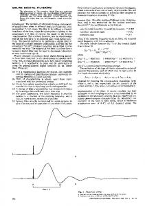
Fig. 1. Non-causal second-order high-pass filter described by (46) and (47) . with cut-off frequency
Matrix
has the form
(47)
. These and satisfy (44). and is of size Note that the output signal is two samples shorter than the input signal . The transfer function of the filter (45) is given by (48) In order that the filter defined by be a low-pass ), the filter with a zero at the Nyquist frequency (i.e., of should be unity at the Nyquist frequency. gain and For the system (45), is found by setting and solving for to obtain . . Hence, for the Equivalently, can be obtained as high-pass filter (45) to have unity Nyquist gain, the coefficients . Then the frequency response is should satisfy given by
The coefficient may be set so that the frequency response has as that frequency a specified cut-off frequency . Defining , one where the frequency response is one half, obtains
For example, setting the cut-off frequency to , gives . This high-pass filter is illustrated in and (a reciprocal Fig. 1. The poles are at pair). This recursive filter is non-causal with a ‘symmetric’ timedomain response (the time-domain response can not be exactly symmetric due to boundary effects in finite-length filtering).
SELESNICK et al.: SIMULTANEOUS LOW-PASS FILTERING AND TOTAL VARIATION DENOISING
1117
We have referred to this recursive filter as a zero-phase filter. That usually means that the filter has a symmetric impulse response. In the context of finite-length signals, the response to , i.e., an impulsed located at an impulse , is not strictly symmetric because the response is of finite length. However, this is always the case when performing finite-length signal filtering, and it does not have a practical impact except for signals that are short relative to the decay-time of the filter. , so it The high-pass filter has a second-order zero at annihilates constant and ramp signals, or any linear combination of these; that is, the output of the filter is identically zero . whenever the input signal is of the form The preceding also is clear from inspection of the mathematical form of in (46). Therefore, the low-pass filter, defined by , exactly preserves polynomial signals of degree 1. B. Higher-Order High-Pass Filter
Fig. 2. Non-causal fourth-order high-pass filter (49) with cut-off frequency and .
Consider the transfer function (49) The filter has a -order zero at , so the frequency is zero at , as are its first derivaresponse can also be written as tives. Also, note that
The numerator of the second term has a zero of order at , so the frequency response has unity gain at , and its first derivatives are zero there. That is, and at the the frequency response is maximally-flat at Nyquist frequency; hence, this is a zero-phase digital Butterworth filter. in (49) is defined by the positive integer The filter and by . The parameter can be set so that the frequency response has a specified cut-off frequency . Setting the gain , gives the at the cut-off frequency to one half, equation
Solving for
gives
The zero-phase high-pass Butterworth filter (49) can be implewhere mented as 1) is a banded matrix of size . is a square symmetric banded matrix of size 2) . ; that is, in addition to 3) Both and have bandwidth the main diagonal, they have diagonals above and below the main diagonal. to an Note that this filter maps an input signal of length . When , we get the highoutput signal of length
Fig. 3. Non-causal fourth-order low-pass filter (50) with cut-off frequency and .
pass filter (48) as a special case. In this case, and , given by (46) and (47), are tridiagonal (a bandwidth of 3). and the cut-off frequency to . Example: Set and has the form The matrix is of size
..
.
..
.
with bandwidth 5. For this example, has non-zero elements in each row. With , one obtains . will be a banded symmetric square matrix are with bandwidth 5. The coefficients of , where lies on diagonal . The resulting fourth-order zero-phase filter is shown in Fig. 2.
1118
IEEE TRANSACTIONS ON SIGNAL PROCESSING, VOL. 62, NO. 5, MARCH 1, 2014
C. Low-Pass Filter The LPF/TVD algorithm provides an estimate, , of the sparse-derivative component and calls for the high-pass filter . The algorithm does not use a low-pass filter. But, to obtain an estimate of the low-pass component, recall that . we need the low-pass filter denoted above as A low-pass filter of this form is trivially performed by subtracting the high-pass filter output from its input. However, note that for the high-pass filter described in Section VI-B, and are rectangular. Consequently, the the matrices output of the high-pass filter is shorter than its input by samples ( at the beginning and at the end). Hence, to implement the low-pass filter, the input signal should likewise be truncated so that the subtraction involves vectors of equal length. Consequently, the low-pass filter can be expressed as where denotes the symmetric truncation of by samples. The low-pass filter matrix, , is therefore given by where is the identity matrix with the first and last rows removed. The matrix is of size . The signal is obtained by deleting the first and last samples from . Based on the high-pass filter (49), the low-pass filter has the transfer function (50) -order zero at . The filter matrix is given by . Example: From the high-pass filter shown in Fig. 2 with , we obtain the low-pass filter illustrated in Fig. 3. The filter . This filter passes can be implemented as ) third-order signals (of the form with no change, except for truncation by two samples at start and end. with a
Fig. 4. LPF/TVD Example 1. Simultaneous low-pass filtering and total variation denoising. From the noisy data, the sparse-derivative and low-pass components are obtained individually. Algorithm parameters: .
VII. EXAMPLES The following examples illustrate the use of the algorithms derived in Sections IV and V for the LPF/TVD and LPF/CSD problems, respectively. A. LPF/TVD Example 1 To illustrate simultaneous low-pass filtering and total-variation denoising, we apply Algorithm 1 (Section IV) to the noisy data shown in Fig. 4. This is the same data used in the first example of [71], where smoothing was performed using a (non-time-invariant) least-squares polynomial approximation. The signal consists of a low-frequency sinusoid, two additive step discontinuities, and additive white Gaussian noise. In order to apply the new algorithm, we must specify a high-pass filter and regularization parameter . We use the fourth-order filter (49) with and cut-off frequency . The parameter was set to 0.8 based on (31). The algorithm was run for 30 iterations. obFig. 4 shows the sparse-derivative component tained from the algorithm. The low-pass component is obtained by low-pass filtering ; it is given by . The total LPF/TVD , shown in the fourth panel of Fig. 4, substantially output,
Fig. 5. LPF/TVD Example 1. The scatter plot verifies that optimality condition (30) is satisfied.
smooths the data while preserving the discontinuities, without introducing Gibbs-like phenomena. The optimality condition (30) is illustrated in Fig. 5 as a , where scatter plot. Each point represents a pair and denote the -th time samples of signals and . lies on the graph of Note that (30) means that if each pair the step function indicated as a dashed line in Fig. 5, then the computed does minimize the objective function in (19). It is seen that most of the points lie on the line , which reflects . the sparsity of
SELESNICK et al.: SIMULTANEOUS LOW-PASS FILTERING AND TOTAL VARIATION DENOISING
As noted in the Introduction, the earlier work in [71] (specifically, the LoPATV algorithm) can also be used to perform the type of processing achieved by the new algorithm. Accordingly, the result shown in Fig. 4 is comparable to the result in [71], which compared favorably to several other methods, as shown therein. However, while the method of [71] calls for the polynomial degree, block length, and overlapping-factor to be specified, the new method calls for the low-pass filter characteristics to be specified (filter order and cut-off frequency). The latter parameters have the benefit of being more in line with conventional filtering practice and notions. To further contrast the new algorithm with LoPATV, we note that the LoPATV algorithms requires that two parameters ( and ) be specified, which raises the issue of how to set these values in order to obtain fast convergence. In contrast, Algorithm 1 formulated in this work does not involve any parameters beyond those in the problem statement (19), and is computationally fast. Thirty iterations of Algorithm 1 takes about 13 milliseconds on a 2013 MacBook Pro (2.5 GHz Intel Core i5) running Matlab R2011a. Run-times reported in subsequent examples are obtained using the same computer.
1119
Fig. 6. LPF/TVD Example 2: NIRS time series data processed with LPF/TVD algorithm. The algorithm removes abrupt changes of the baseline and transient . artifacts. Algorithm parameters:
B. LPF/TVD Example 2 Fig. 6 illustrates the use of Algorithm 1 on 304 seconds of NIRS time series data. The data has a sampling rate of 6.25 sam). The data used for this example ples/second (length is the record of the time-dependent NIRS light-intensity level, for one channel in a multi-probe physiological measurement session. All of the light-emitting and -receiving optodes, where an optode is the optical analogue of an EEG electrode, were located on the scalp of an adult male research-study subject. The terms ‘source’ and ‘detector’ are used to refer to a light-emitting optode and a light-receiving optode, respectively, and a measurement channel is defined by specifying a particular source-detector pair. For example, for the channel considered here, the source and detector were located on the subject’s scalp over the back of the head. NIRS data from measurements of this type are susceptible to subject-motion artifacts, as indicated in Section I-B. In some cases, and as seen most strikingly at approximately the 80-second mark, motion can cause a change in optode-skin contact sufficient to produce an abrupt, permanent shift in the baseline value. It can be observed that the TVD component produced by the algorithm successfully captures the discontinuities and transient artifacts present in the data. The LPF/TVD algorithm was run for 30 iterations with a total run time of 30 milliseconds. To concretely illustrate the benefits of LPF/TVD in comparison with LTI filtering alone, we consider the problem of detrending (baseline removal). When a zero-phase LTI highpass filter is used to remove the baseline of the data shown in Fig. 6, we obtain the detrended signal illustrated in Fig. 7. The abrupt jumps in the data produce transients in the detrended data—an unavoidable consequence of LTI filtering. However, if the TV component obtained using LPF/TVD is subtracted from the data prior to LTI high-pass filtering, then the transients are greatly reduced, as illustrated in the figure. The near-elimination of the transients is possible because the LPF/TVD algorithm is nonlinear. A further benefit of LPF/TVD processing is revealed in the frequency domain. In particular, the Welch periodogram in Fig. 7 shows that LPF/TVD preprocessing reduces the strong,
Fig. 7. LPF/TVD Example 2. Detrending by high-pass filtering and by LPF/TVD prior to high-pass filtering. In the periodogram, LPF/TVD uncovers a signal component at frequency 0.32 Hz which is otherwise obscured by the broad low-frequency energy due to strong transients.
broad low-frequency energy due to the transients. Consequently, a signal component at about 0.32 Hz, which in the HPF
1120
IEEE TRANSACTIONS ON SIGNAL PROCESSING, VOL. 62, NO. 5, MARCH 1, 2014
Fig. 8. LPF/CSD Example 1. Comparison of convergence of Algorithm 1 (LPF/TVD) and Algorithm 2 (LPF/CSD).
result is obscured by the broad power spectrum arising from the transients, is unambiguously revealed. Notably, this lies within the range of typical human respiration frequencies (12–20 cycles/min). The respiratory rhythm is frequently observed in data from NIRS physiological measurements [3], [8], and PSD analysis of relatively artifact-free channels from the same recording session indicate that the participant’s respiratory frequency was indeed about 0.32 Hz. This example shows how the LPF/TVD method can be used to improve the effectiveness of LTI filtering and spectral analysis.
Fig. 9. LPF/CSD Example 2. Near infrared spectroscopic (NIRS) data and LPF/CSD processing. The method simultaneously performs low-pass filtering and sparse signal denoising.
We remark that the LoPATV algorithm [71] (which performs LPF/TVD-type processing) requires the specification of two parameters. Hence, it is even more affected by the issues of (1) parameter tuning for fast convergence and (2) fastest achievable convergence.
C. LPF/CSD Example 1
D. LPF/CSD Example 2
Note that the LPF/CSD problem (32) generalizes the LPF/TVD problem (19). Specifically, the LPF/TVD problem is in (32). Hence, Algorithm 2 (Section V) recovered with can be used to solve the LPF/TVD problem. For example, it can be used to perform the processing illustrated in Fig. 6 for which we used Algorithm 1. Consequently, it may appear that Algorithm 1 is unnecessary. However, in the following, we demonstrate two advantages of Algorithm 1, in comparison with Algorithm 2, for solving the LPF/TVD problem. In order to compare the convergence behavior of Algorithms 1 and 2, we apply both of them to the data shown in Fig. 6 (“Original data” in gray). The Algorithm 2 result is visually indistinguishable from that obtained with Algorithm 1, so we do not illustrate it separately. The cost function history of each algorithm is illustrated in Fig. 8. Algorithm 1 converges well within 30 iterations. Note, however, that Algorithm 2 requires the user to specify a param, which can be interpreted as a type of step-size paeter rameter. As illustrated in Fig. 8, the convergence behavior of , the algorithm initially Algorithm 2 depends on . For converges quickly but has very slow long-term convergence. , the algorithm has better long-term convergence, For but poor initial convergence. Note that Algorithm 1 converges much faster than Algorithm 2, regardless of . In comparison with Algorithm 2, Algorithm 1 has two advantages. First, it does not require the user to specify a parameter . Second, it often converges faster regardless of what value of is used for Algorithm 2. On the other hand, Algorithm 2 solves the more general problem of LPF/CSD and can therefore perform processing that is not possible with Algorithm 1.
To illustrate simultaneous low-pass filtering and compound sparse denoising (LPF/CSD), we have obtained data from a dynamic tissue-simulating phantom [9], while varying the strength of its absorption for NIR light in a manner that emulates the hemodynamic response of a human brain to intermittently delivered stimuli. Fig. 9 illustrates data acquired by the system. The signal is of length 4502 samples, with a sampling rate of 1.25 samples/second and an observation time of 3602 seconds. The ‘hemodynamic’ pulses are observed in the presence of unavoidable low-frequency background processes and wideband noise. The signal of interest and its derivative are sparse relative to the low-frequency background signal and noise. For the illustrated measurement channel, the noise standard deviation is greater than 10% of the largest-magnitude hemodynamic pulse; this is not an uncommon noise level for physiological NIRS data [3]. Algorithm 2 simultaneously estimates and separates the low-pass background signal and the hemodynamic pulses, as illustrated in Fig. 9. For this computation, 50 iterations of the algorithm were performed, in a time of 70 milliseconds. The pulses are illustrated in detail in Fig. 10. Note that the shapes of the pulses are well preserved, in contrast to the commonly observed amplitude-reducing, edge-spreading, and plateau-rounding, of LTI filtering alone (see Fig. 10(b)). For comparison, Fig. 10 illustrates the output of a band-pass filter (BPF) applied to the same noisy data. Note that the BPF signal exhibits both more baseline drift and more noise than the CSD component produced by LPF/CSD processing. In particular, the BPF obscures the amplitude of the hemodynamic pulses relative to the baseline. While the band-edges of the BPF can be adjusted to obtain a different BPF signal from the one
SELESNICK et al.: SIMULTANEOUS LOW-PASS FILTERING AND TOTAL VARIATION DENOISING
1121
peaks. The result was obtained using software by the author at http://www.mathworks.com/matlabcentral/fileexchange/. Finally, the result of LPF/TVD processing is also shown in Fig. 10. It can be seen that the TVD component produced by Algorithm 1 is similar to the CSD component produced by Algorithm 2; however, it exhibits baseline drift. Algorithm 1 cannot achieve a baseline value of zero due to the absence in (19) of term that is present in (32). the E. LPF/CSD Example 3
Fig. 10. LPF/CSD Example 2. For the data in Fig. 9, the output of a bandpass filter (BPF), a de-spiking algorithm [54], and the TVD component obtained using LPF/TVD are shown for comparison with LPF/CSD. (a) Full duration of the data time series. (b) Expanded view of a brief portion of the time series.
shown here, these adjustments will either increase the residual noise level, increase the baseline drift, or further distort the shape of the hemodynamic pulses. For further comparison, Fig. 10 also illustrates the output of a recent de-spiking algorithm [54]; see also [48]. The algorithm is based on clustering in phase-space, wherein the state vector consists of both the value of the signal and its derivative. This de-spiking algorithm simultaneously uses both the signal value and its derivative, like the LPF/CSD approach derived here. However, it does not explicitly account for the presence of a low-pass component. It can be observed that some false peaks occur and that residual noise remains on the crests of the
The LPF/CSD approach can also be used for artifact reduction, as illustrated in Fig. 11. The data is a 300-second NIRS time series from the same experimental measurement as in LPF/TVD Example 2 above. However, for the channel considered here, the source and detector were located on the subject’s forehead in the vicinity of his left eye. This makes the data susceptible to motion artifacts due to eye blinks (in addition to all other sources of motion artifact that ordinarily are present). The data is corrupted by transients of variable amplitude, width, and shape. The CSD component was obtained using 50 iterations of Algorithm 2 with a total run-time of 30 milliseconds. Fig. 11 displays a 100-second interval of the 300-second signal, to more clearly show the details of the data. The CSD component captures the transients with reasonable accuracy while maintaining a baseline of zero. Subtraction of the CSD component from the original data demonstrates that the algorithm has largely removed the artifacts while leaving the (physiological) oscillatory behavior intact. The benefit can also be seen in the frequency domain. When the CSD component is subtracted from the data, the periodogram shows a broad peak in the 1.0–1.2 Hz band. Notably, this lies within the range of typical human cardiac (i.e., heartbeat) frequencies (60–100 cycles/min). The cardiac rhythm is frequently observed in data from NIRS physiological measurements [3], [8], and PSD analysis of relatively artifact-free channels from the same recording session indicate that the participant’s cardiac frequency was indeed approximately 1.1 Hz. In the periodogram of the original data, this peak is obscured by the broad-band energy of the transient artifacts. For comparison, Fig. 12 illustrates the output of two recent algorithms, the de-spiking algorithm of [54] and the motion artifact reduction algorithms of [36]. This second method, which was implemented using the NAP software application written by the authors of [36], [37], identifies outliers in a high-pass filtered version of the time series, based on a user-specified z-score threshold. These values are then replaced: a simple linear interpolation is used for ‘spikes’ (i.e., artifacts briefer than a user-specified maximum duration); for ‘ripples’ (i.e., artifacts for which the number of consecutive data values having supra-threshold z-scores exceeds a user-specified minimum), the data are approximated with piecewise-continuous cubic polynomials, and the corrected data are the differences between the original data and the best-fitting cubics. Elsewhere in the time series, the original data are not modified. It can be observed in Fig. 12 that the algorithms of [36], [54] successfully identify high-amplitude spikes, but yield restored time-series that are less regular than the proposed method. Both methods [36], [54] are based on a two-step procedure: first identify spikes (or ripples); second, interpolate to fill in the
1122
IEEE TRANSACTIONS ON SIGNAL PROCESSING, VOL. 62, NO. 5, MARCH 1, 2014
TABLE I
and non-artifact data points, and is flexible in terms of the types of artifacts it can handle. F. Run-Times The run-times from the examples of Algorithm 1 and Algorithm 2 for LPF/TVD and LPF/CSD respectively, are summarized in Table I. VIII. CONCLUSION
Fig. 11. LPF/CSD Example 3. Removal of artifacts from a NIRS time series by LPF/CSD processing.
Sparsity-based signal processing methods are now highly developed, but in practice LTI filtering still is predominant for noise reduction for 1-D signals. This paper presents a convex optimization approach for combining low-pass filtering and sparsity-based denoising to more effectively filter (denoise) a wider class of signals. The first algorithm, solving the LPF/TVD problem (19), assumes that the signal of interest is composed of a low-frequency component and a sparse-derivative component. The second algorithm, solving the LPF/CSD problem (32), assumes the second component is both sparse and has a sparse derivative. Both algorithms draw on the computational efficiency of fast solvers for banded linear systems, available for example as part of LAPACK [4]. The problem formulation and algorithms described in this paper can be extended in several ways. As in [71], enhanced norm by regularsparsity can be achieved by replacing the izers that promote sparsity more strongly, such as the pseudo, or by reweighted [18], greedy [58], norm etc. In addition, in place of total variation, higher-order or generalized total variation can be used [56]. The use of LTI filters other than a low-pass filter may also be useful; for example, the use of band-pass or notch filters may be appropriate for specific signals. It is envisioned that more general forms of the approach taken in this paper will demand more powerful optimization algorithms than those employed here. In particular, recently developed optimization frameworks based on proximity operators [14], [20], [26], [28], [63], [66] are specifically geared to problems involving sums of non-smooth convex functions (i.e., compound regularization). ACKNOWLEDGMENT
Fig. 12. LPF/CSD Example 3. Result of NAP [36] and de-spiking [54].
gaps. In addition, neither method attempts to identify or correct additive steps in the data, and hence they are not effective for examples where LPF/TVD can be used. In contrast, the proposed method consists of a single problem formulation, which does not rely on a segmentation of the time series into artifact
The authors gratefully acknowledge Justin R. Estepp (Air Force Research Laboratory, Wright-Patterson AFB, OH) and Sean M. Weston (Oak Ridge Institute for Science and Education, TN) for providing experimental data used in LPF/TVD Example 2 and LPF/CSD Example 3. REFERENCES [1] M. V. Afonso, J. M. Bioucas-Dias, and M. A. T. Figueiredo, “An augmented Lagrangian approach to linear inverse problems with compound regularization,” in Proc. IEEE Int. Conf. Image Process., Sep. 2010, pp. 4169–4172.
SELESNICK et al.: SIMULTANEOUS LOW-PASS FILTERING AND TOTAL VARIATION DENOISING
[2] M. V. Afonso, J. M. Bioucas-Dias, and M. A. T. Figueiredo, “Fast image recovery using variable splitting and constrained optimization,” IEEE Trans. Image Process., vol. 19, no. 9, pp. 2345–2356, Sep. 2010. [3] R. Al abdi, H. L. Graber, Y. Xu, and R. L. Barbour, “Optomechanical imaging system for breast cancer detection,” J. Opt. Soc. Amer. A, vol. 28, no. 12, pp. 2473–2493, Dec. 2011. [4] E. Anderson, Z. Bai, C. Bischof, J. Demmel, J. Dongarra, J. Du Croz, A. Greenbaum, S. Hammarling, A. McKenney, S. Ostrouchov, and D. Sorensen, LAPACK’s User’s Guide. Philadelphia, PA, USA: SIAM, 1992 [Online]. Available: http://www.netlib.org/lapack [5] J.-F. Aujol, G. Aubert, L. Blanc-Féraud, and A. Chambolle, “Image decomposition into a bounded variation component and an oscillating component,” J. Math. Imag. Vis., vol. 22, pp. 71–88, 2005. [6] J.-F. Aujol, G. Gilboa, T. Chan, and S. J. Osher, “Structure-texture image decomposition—Modeling, algorithms, and parameter selection,” Int. J. Comput. Vis., vol. 67, no. 1, pp. 111–136, Apr. 2006. [7] F. Bach, R. Jenatton, J. Mairal, and G. Obozinski, “Optimization with sparsity-inducing penalties,” Found. Trends Mach. Learn., vol. 4, no. 1, pp. 1–106, 2012. [8] R. L. Barbour, H. L. Graber, Y. Pei, S. Zhong, and C. H. Schmitz, “Optical tomographic imaging of dynamic features of dense-scattering media,” J. Opt. Soc. Amer. A, vol. 18, no. 12, pp. 3018–3036, Dec. 2001. [9] R. L. Barbour, H. L. Graber, Y. Xu, Y. Pei, C. H. Schmitz, D. S. Pfeil, A. Tyagi, R. Andronica, D. C. Lee, S.-L. S. Barbour, J. D. Nichols, and M. E. Pflieger, “A programmable laboratory testbed in support of evaluation of functional brain activation and connectivity,” IEEE Trans. Neural Syst. Rehabil. Eng., vol. 20, no. 2, pp. 170–183, Mar. 2012. [10] J. Bect, L. Blanc-Féraud, G. Aubert, and A. Chambolle, T. Pajdla and J. Matas, Eds., “A -unified variational framework for image restoration,” in Proc. Eur. Conf. Comput. Vis., Lecture Notes in Comput. Sci., 2004, vol. 3024, pp. 1–13. [11] J. M. Bioucas-Dias and M. A. T. Figueiredo, “An iterative algorithm for linear inverse problems with compound regularizers,” in Proc. IEEE Int. Conf. Image Process., Oct. 2008, pp. 685–688. [12] S. Boyd, N. Parikh, E. Chu, B. Peleato, and J. Eckstein, “Distributed optimization and statistical learning via the alternating direction method of multipliers,” Found. Trends Mach. Learn., vol. 3, no. 1, pp. 1–122, 2011. [13] K. Bredies, K. Kunisch, and T. Pock, “Total generalized variation,” SIAM J. Imag. Sci., vol. 3, no. 3, pp. 492–526, 2010. [14] L. M. Briceño-Arias and P. L. Combettes, “A monotone+skew splitting model for composite monotone inclusions in duality,” SIAM J. Optim., vol. 21, no. 4, pp. 1230–1250, Oct. 2011. [15] L. M. Briceño-Arias, P. L. Combettes, J.-C. Pesquet, and N. Pustelnik, “Proximal method for geometry and texture image decomposition,” in Proc. IEEE Int. Conf. Image Process., 2010, pp. 2721–2724. [16] V. Bruni and D. Vitulano, “Wavelet-based signal de-noising via simple singularities approximation,” Signal Process., vol. 86, no. 4, pp. 859–876, Apr. 2006. [17] C. S. Burrus, R. A. Gopinath, and H. Guo, Introduction to Wavelets and Wavelet Transforms. Englewood Cliffs, NJ, USA: Prentice-Hall, 1997. [18] E. J. Candès, M. B. Wakin, and S. Boyd, “Enhancing sparsity by reweighted l1 minimization,” J. Fourier Anal. Appl., vol. 14, no. 5, pp. 877–905, Dec. 2008. [19] A. Chambolle and P.-L. Lions, “Image recovery via total variation minimization and related problems,” Numer. Math., vol. 76, pp. 167–188, 1997. [20] A. Chambolle and T. Pock, “A first-order primal-dual algorithm for convex problems with applications to imaging,” J. Math. Vis., vol. 40, no. 1, pp. 120–145, 2011. [21] T. F. Chan, S. Osher, and J. Shen, “The digital TV filter and nonlinear denoising,” IEEE Trans. Image Process., vol. 10, no. 2, pp. 231–241, Feb. 2001. [22] S. Chen, D. L. Donoho, and M. A. Saunders, “Atomic decomposition by basis pursuit,” SIAM J. Sci. Comput., vol. 20, no. 1, pp. 33–61, 1998. [23] R. R. Coifman and D. L. Donoho, “Translation-invariant de-noising,” in Wavelet and Statistics, A. Antoniadis and G. Oppenheim, Eds. New York, NY, USA: Springer-Verlag, 1995, pp. 125–150. [24] P. L. Combettes and J.-C. Pesquet, “Proximal thresholding algorithm for minimization over orthonormal bases,” SIAM J. Optim., vol. 18, no. 4, pp. 1351–1376, 2008. [25] P. L. Combettes and J.-C. Pesquet, “Proximal splitting methods in signal processing,” in Fixed-Point Algorithms for Inverse Problems in Science and Engineering, H. H. Bauschke, Ed. et al. New York, NY, USA: Springer-Verlag, 2011, pp. 185–212.
1123
[26] P. L. Combettes and J.-C. Pesquet, “Primal-dual splitting algorithm for solving inclusions with mixtures of composite, Lipschitzian, and parallel-sum type monotone operators,” Set-Valued Variat. Anal., vol. 20, no. 2, pp. 307–330, Jun. 2012. [27] L. Condat, “A direct algorithm for 1-D total variation denoising,” IEEE Signal Process. Lett., vol. 20, no. 11, pp. 1054–1057, Nov. 2013. [28] L. Condat, “A primal-dual splitting method for convex optimization involving Lipschitzian, proximable and linear composite terms,” J. Optim. Theory Appl., vol. 158, no. 2, pp. 460–479, 2013. [29] M. S. Crouse, R. D. Nowak, and R. G. Baraniuk, “Wavelet-based signal processing using hidden Markov models,” IEEE Trans. Signal Process., vol. 46, no. 4, pp. 886–902, Apr. 1998. [30] V. R. Dantham, S. Holler, V. Kolchenko, Z. Wan, and S. Arnold, “Taking whispering gallery-mode single virus detection and sizing to the limit,” Appl. Phys. Lett., vol. 101, no. 4, p. 043704, 2012. [31] L. Daudet and B. Torrésani, “Hybrid representations for audiophonic signal encoding,” Signal Process., vol. 82, no. 11, pp. 1595–1617, Nov. 2002. [32] D. L. Donoho, “De-noising by soft-thresholding,” IEEE Trans. Inf. Theory, vol. 41, no. 3, pp. 613–627, May 1995. [33] S. Durand and M. Nikolova, “Denoising of frame coefficients using data-fidelity term and edge-preserving regularization,” Multiscale Model. Simul., vol. 6, no. 2, pp. 547–576, 2007. [34] M. Elad, Sparse and Redundant Representations: From Theory to Applications in Signal and Image Processing. New York, NY, USA: Springer, 2010. [35] E. Esser, X. Zhang, and T. F. Chan, “A general framework for a class of first order primal-dual algorithms for convex optimization in imaging science,” SIAM J. Imag. Sci., vol. 3, no. 4, pp. 1015–1046, 2010. [36] T. Fekete, D. Rubin, J. M. Carlson, and L. R. Mujica-Parodi, “The NIRS analysis package: Noise reduction and statistical inference,” PLoS ONE, vol. 6, no. 9, p. e24322, 2011. [37] T. Fekete, D. Rubin, J. M. Carlson, and L. R. Mujica-Parodi, “A stand-alone method for anatomical localization of NIRS measurements,” Neuroimage, vol. 56, no. 4, pp. 2080–2088, Jun. 15, 2011. [38] M. Figueiredo, J. Bioucas-Dias, and R. Nowak, “Majorization-minimization algorithms for wavelet-based image restoration,” IEEE Trans. Image Process., vol. 16, no. 12, pp. 2980–2991, Dec. 2007. [39] M. Figueiredo, J. Bioucas-Dias, J. P. Oliveira, and R. D. Nowak, “On total-variation denoising: A new majorization-minimization algorithm and an experimental comparison with wavelet denoising,” in Proc. IEEE Int. Conf. Image Process., 2006, pp. 2633–2636. [40] J. Friedman, T. Hastie, H. Höfling, and R. Tibshirani, “Pathwise coordinate optimization,” Ann. Appl. Statist., vol. 1, no. 2, pp. 302–332, 2007. [41] J.-J. Fuchs, “On sparse representations in arbitrary redundant bases,” IEEE Trans. Inf. Theory, vol. 50, no. 6, pp. 1341–1344, 2004. [42] J. J. Fuchs, “Identification of real sinusoids in noise, the Global Matched Filter approach,” in Proc. 15th IFAC Symp. Syst. Identificat., Saint-Malo, France, Jul. 2009, pp. 1127–1132. [43] D. Geman and G. Reynolds, “Constrained restoration and the recovery of discontinuities,” IEEE Trans. Pattern Anal. Mach. Intell., vol. 14, no. 3, pp. 367–383, Mar. 1992. [44] A. Gholami and S. M. Hosseini, “A balanced combination of Tikhonov and total variation regularizations for reconstruction of piecewise-smooth signals,” Signal Process., vol. 93, no. 7, pp. 1945–1960, 2013. [45] J. R. Gilbert, C. Moler, and R. Schreiber, “Sparse matrices in MATLAB: Design and implementation,” SIAM J. Matrix. Anal. Appl., vol. 13, no. 1, pp. 333–356, Jan. 1992. [46] T. Goldstein and S. Osher, “The split Bregman method for L1-regularized problems,” SIAM J. Imag. Sci., vol. 2, no. 2, pp. 323–343, 2009. [47] G. H. Golub and C. F. Van Loan, Matrix Computations. Baltimore, MD, USA: The Johns Hopkins Univ. Press, 1996. [48] D. Goring and V. Nikora, “Despiking acoustic Doppler velocimeter data,” J. Hydraul. Eng., vol. 128, no. 1, pp. 117–126, Jan. 2002. [49] M. Grasmair, “The equivalence of the taut string algorithm and BVregularization,” J. Math. Imag. Vis., vol. 27, no. 1, pp. 59–66, Jan. 2007. [50] F. Gustafsson, “Determining the initial states in forward-backward filtering,” IEEE Trans. Signal Process., vol. 44, no. 4, pp. 988–992, Apr. 1996. [51] C. Habermehl, S. Holtze, J. Steinbrink, S. P. Koch, H. Obrig, J. Mehnert, and C. H. Schmitz, “Somatosensory activation of two fingers can be discriminated with ultrahigh-density diffuse optical tomography,” NeuroImage, vol. 59, pp. 3201–3211, 2012. [52] Y. Hu and M. Jacob, “Higher degree total variation (HDTV) regularization for image recovery,” IEEE Trans. Image Process., vol. 21, no. 5, pp. 2559–2571, May 2012.
1124
[53] A. Hyvärinen, “Sparse code shrinkage: Denoising of non-Gaussian data by maximum likelihood estimation,” Neural Comput., vol. 11, pp. 1739–1768, 1999. [54] M. R. Islam and D. Z. Zhu, “Kernel density-based algorithm for despiking ADV data,” J. Hydraul. Eng., vol. 139, no. 7, pp. 785–793, Jul. 2013. [55] L. Jacques, L. Duval, C. Chaux, and G. Peyré, “A panorama on multiscale geometric representations, intertwining spatial, directional and frequency selectivity,” Signal Process., vol. 91, no. 12, pp. 2699–2730, Dec. 2011. [56] F. I. Karahanoglu, I. Bayram, and D. Van De Ville, “A signal processing approach to generalized 1-d total variation,” IEEE Trans. Signal Process., vol. 59, no. 11, pp. 5265–5274, Nov. 2011. [57] V. Katkovnik, K. Egiazarian, and J. Astola, Local Approximation Techniques in Signal and Image Processing. Bellingham, WA, USA: SPIE Press, 2006. [58] I. Kozlov and A. Petukhov, , W. Freeden, Ed. et al., “Sparse solutions of underdetermined linear systems,” in Handbook of Geomathematics. New York, NY, USA: Springer, 2010. [59] S.-H. Lee and M. G. Kang, “Total variation-based image noise reduction with generalized fidelity function,” IEEE Signal Process. Lett., vol. 14, no. 11, pp. 832–835, Nov. 2007. [60] S. Mallat, A Wavelet Tour of Signal Processing. New York, NY, USA: Academic, 1998. [61] J. E. W. Mayhew, S. Askew, Y. Zheng, J. Porrill, G. W. M. Westby, P. Redgrave, D. M. Rector, and R. M. Harper, “Cerebral vasomotion: A 0.1-Hz oscillation in reflected light imaging of neural activity,” NeuroImage, vol. 4, pp. 183–193, 1996. [62] T. W. Parks and C. S. Burrus, Digital Filter Design. New York, NY, USA: Wiley, 1987. [63] J.-C. Pesquet and N. Pustelnik, “A parallel inertial proximal optimization method,” Pacific J. Optim., vol. 8, no. 2, pp. 273–305, Apr. 2012. [64] J. Portilla, V. Strela, M. J. Wainwright, and E. P. Simoncelli, “Image denoising using scale mixtures of Gaussians in the wavelet domain,” IEEE Trans. Image Process., vol. 12, no. 11, pp. 1338–1351, Nov. 2003. [65] W. H. Press, S. A. Teukolsky, W. T. Vetterling, and B. P. Flannery, Numerical Recipes in C: The Art of Scientific Computing, 2nd ed. Cambridge, U.K.: Cambridge Univ. Press, 1992. [66] H. Raguet, J. Fadili, and G. Peyré, “Generalized forward-backward splitting,” Jan. 2012 [Online]. Available: http://arxiv.org/abs/1108. 4404 [67] B. D. Rao, K. Engan, S. F. Cotter, J. Palmer, and K. Kreutz-Delgado, “Subset selection in noise based on diversity measure minimization,” IEEE Trans. Signal Process., vol. 51, no. 3, pp. 760–770, Mar. 2003. [68] L. Rudin, S. Osher, and E. Fatemi, “Nonlinear total variation based noise removal algorithms,” Physica D, vol. 60, pp. 259–268, 1992. [69] I. W. Selesnick, “Resonance-based signal decomposition: A new sparsity-enabled signal analysis method,” Signal Process., vol. 91, no. 12, pp. 2793–2809, 2011. [70] I. W. Selesnick, “Simultaneous polynomial approximation and total variation denoising,” in Proc. IEEE Int. Conf. Acoust., Speech, Signal Process. (ICASSP), May 2013, pp. 5944–5948. [71] I. W. Selesnick, S. Arnold, and V. R. Dantham, “Polynomial smoothing of time series with additive step discontinuities,” IEEE Trans. Signal Process., vol. 60, no. 12, pp. 6305–6318, Dec. 2012. [72] J.-L. Starck, M. Elad, and D. Donoho, “Image decomposition via the combination of sparse representation and a variational approach,” IEEE Trans. Image Process., vol. 14, no. 10, pp. 1570–1582, Oct. 2005. [73] R. Tibshirani, “Regression shrinkage and selection via the lasso,” J. Roy. Statist. Soc., Ser. B, vol. 58, no. 1, pp. 267–288, 1996. [74] J. A. Tropp, “Just relax: Convex programming methods for identifying sparse signals in noise,” IEEE Trans. Inf. Theory, vol. 52, no. 3, pp. 1030–1051, Mar. 2006. [75] L. A. Vese and S. Osher, “Image denoising and decomposition with total variation minimization and oscillatory functions,” J. Math. Imag. Vis., vol. 20, pp. 7–18, 2004. [76] B. C. Vu, “A splitting algorithm for dual monotone inclusions involving cocoercive operators,” Adv. Comp. Math, vol. 38, no. 3, pp. 667–681, Nov. 2013.
IEEE TRANSACTIONS ON SIGNAL PROCESSING, VOL. 62, NO. 5, MARCH 1, 2014
[77] B. R. White, A. Q. Bauer, A. Z. Snyder, B. L. Schlaggar, J.-M. Lee, and J. P. Culver, “Imaging of functional connectivity in the mouse brain,” PLoS ONE, vol. 6, no. 1, p. e16322, 2011. [78] C. Wu and X. Tai, “Augmented Lagrangian method, dual methods, and split Bregman iteration for ROF, vectorial TV, and high order models,” SIAM J. Imag. Sci., vol. 3, no. 3, pp. 300–339, 2010.
Ivan W. Selesnick (S’91–M’98–SM’08) received the B.S., M.E.E., and Ph.D. degrees in electrical engineering in 1990, 1991, and 1996 from Rice University, Houston, TX. In 1997, he was a visiting professor at the University of Erlangen-Nurnberg, Germany. He then joined the Department of Electrical and Computer Engineering, NYU Polytechnic School of Engineering, New York (then Polytechnic University), where he is associate Professor. His current research interests are in the area of digital signal and image processing, wavelet-based signal processing, sparsity techniques, and biomedical signal processing. He has been an associate editor for the IEEE TRANSACTIONS ON IMAGE PROCESSING, IEEE SIGNAL PROCESSING LETTERS, and IEEE TRANSACTIONS ON SIGNAL PROCESSING.
Harry L. Graber (M’95) received the A.B. degree in chemistry from the Washington University, St. Louis, MO, in 1983, and the Ph.D. degree in physiology and biophysics from SUNY Downstate Medical Center, Brooklyn, NY, in 1998. He subsequently became a Research Associate (1998) and then a Research Assistant Professor (2001) at SUNY Downstate Medical Center. Since 2001 he also has been the Senior Applications Specialist for NIRx Medical Technologies. His research interests include diffuse optical imaging algorithms, and application of feature extraction and time-series analysis methods for interpretation of biological signals.
Douglas S. Pfeil received the B.S. degree in biochemistry from Lehigh University, Bethlehem, PA, in 2007. He is an M.D./Ph.D. candidate in the Molecular and Cellular Biology Program at SUNY Downstate Medical Center, Brooklyn, NY. His research interests include near infrared imaging of the human and primate brain, particularly changes that can occur during surgery. Previously, he studied the molecular biology of nerve cell growth cones in the Wadsworth laboratory at Robert Wood Johnson University Hospital.
Randall L. Barbour received the Ph.D. degree in biochemistry from Syracuse University, Syracuse, NY, in 1981. This was followed by a postdoctoral fellowship in Laboratory Medicine at SUNY at Buffalo. He is currently Professor of Pathology at SUNY Downstate Medical Center, and Research Professor of Electrical Engineering at Polytechnic University, Brooklyn, NY. He is an originator of the field of diffuse optical tomography and is co-founder of NIRx Medical Technologies, LLC. He has an extensive background in a broad range of medical and scientific and technical fields.