Simultaneous Object Recognition and Segmentation by Image

Simultaneous Object Recognition and Segmentation by Image Exploration Vittorio Ferrari1, Tinne Tuytelaars2 , and Luc Van Gool1,2 1

Computer Vision Group (BIWI), ETH Z¨ urich, Switzerland 2 ESAT-PSI, University of Leuven, Belgium

Abstract. Methods based on local, viewpoint invariant features have proven capable of recognizing objects in spite of viewpoint changes, occlusion and clutter. However, these approaches fail when these factors are too strong, due to the limited repeatability and discriminative power of the features. As additional shortcomings, the objects need to be rigid and only their approximate location is found. We present an object recognition approach which overcomes these limitations. An initial set of feature correspondences is first generated. The method anchors on it and then gradually explores the surrounding area, trying to construct more and more matching features, increasingly farther from the initial ones. The resulting process covers the object with matches, and simultaneously separates the correct matches from the wrong ones. Hence, recognition and segmentation are achieved at the same time. Only very few correct initial matches suffice for reliable recognition. Experimental results on still images and television news broadcasts demonstrate the stronger power of the presented method in dealing with extensive clutter, dominant occlusion, large scale and viewpoint changes. Moreover non-rigid deformations are explicitly taken into account, and the approximative contours of the object are produced. The approach can extend any viewpoint invariant feature extractor.

1

Introduction

The modern trend in object recognition has abandoned model-based approaches (e.g. [2]), which require a 3D model of the object as input, in favor of appearancebased ones, where some example images suffice. Two kinds of appearance-based methods exist: global and local. Global methods build an object representation by integrating information over an entire image (e.g [4,17,27]), and are therefore very sensitive to background clutter and partial occlusion. Hence, global methods only consider test images without background, or necessitate a prior segmentation, a task which has proven extremely difficult. Additionally, robustness to large viewpoint changes is hard to achieve, because the global object appearance varies in a complex and unpredictable way (the object’s geometry is unknown). Local methods counter problems due to clutter and occlusion by representing images as a

This research was supported by EC project VIBES, the Fund for Scientific Research Flanders, and the IST Network of Excellence PASCAL.

J. Ponce et al. (Eds.): Toward Category-Level Object Recognition, LNCS 4170, pp. 145–169, 2006. c Springer-Verlag Berlin Heidelberg 2006

146

V. Ferrari, T. Tuytelaars, and L. Van Gool

collection of features extracted based on local information only (e.g. [25]). After the influential work of Schmid [24], who proposed the use of rotation-invariant features, there has been important evolution. Feature extractors have appeared [12,14] which are invariant also under scale changes, and more recently recognition under general viewpoint changes has become possible, thanks to extractors adapting the complete affine shape of the feature to the viewing conditions [1,13,15,23,31,30]. These affine invariant features are particularly significant: even though the global appearance variation of 3D objects is very complex under viewpoint changes, it can be approximated by simple affine transformations on a local scale, where each feature is approximately planar (a region). Local invariant features are used in many recent works, and provide the currently most successful paradigm for object recognition (e.g. [12,15,18,21,30]). In the basic common scheme a number of features are extracted independently from both a model and a test image, then characterized by invariant descriptors and finally matched. In spite of their success, the robustness and generality of these approaches are limited by the repeatability of the feature extraction, and the difficulty of matching correctly, in the presence of large amounts of clutter and challenging viewing conditions. Indeed, large scale or viewpoint changes considerably lower the probability that any given model feature is re-extracted in the test image. Simultaneously, occlusion reduces the number of visible model features. The combined effect is that only a small fraction of model features has a correspondence in the test image. This fraction represents the maximal number of features that can be correctly matched. Unfortunately, at the same time extensive clutter gives rise to a large number of non-object features, which disturb the matching process. As a final outcome of these combined difficulties, only a few, if any, correct matches are produced. Because these often come together with many mismatches, recognition tends to fail. Even in easier cases, to suit the needs for repeatability in spite of viewpoint changes, only a sparse set of distinguished features [18] are extracted. As a result, only a small portion of the object is typically covered with matches. Densely covering the visible part of the object is desirable, as it increases the evidence for its presence, which results in higher detection power. Moreover, it would allow to find the contours of the object, rather than just its location. The image exploration approach. In this chapter we tackle these problems with a new, powerful technique to match a model view to the test image which no longer relies solely on matching viewpoint invariant features. We start by producing an initial large set of unreliable region correspondences, so as to maximize the number of correct matches, at the cost of introducing many mismatches. Additionally, we generate a grid of regions densely covering the model image. The core of the method then iteratively alternates between expansion phases and contraction phases. Each expansion phase tries to construct regions corresponding to the coverage ones, based on the geometric transformation of nearby existing matches. Contraction phases try to remove incorrect matches, using filters that tolerate non-rigid deformations.

Simultaneous Object Recognition and Segmentation by Image Exploration

147

This scheme anchors on the initial matches and then looks around them trying to construct more. As new matches arise, they are exploited to construct even more, in a process which gradually explores the test image, recursively constructing more and more matches, increasingly farther from the initial ones. At each iteration, the presence of the new matches helps the filter taking better removal decisions. In turn, the cleaner set of matches makes the next expansion more effective. As a result, the number, percentage and extent of correct matches grow with every iteration. The two closely cooperating processes of expansion and contraction gather more evidence about the presence of the object and separate correct matches from wrong ones at the same time. Hence, they achieve simultaneous recognition and segmentation of the object. By constructing matches for the coverage regions, the system succeeds in covering also image areas which are not interesting for the feature extractor or not discriminative enough to be correctly matched by traditional techniques. During the expansion phases, the shape of each new region is adapted to the local surface orientation, allowing the exploration process to follow curved surfaces and deformations (e.g. a folded magazine). The basic advantage of our approach is that each single correct initial match can expand to cover a smooth surface with many correct matches, even when starting from a large number of mismatches. This leads to filling the visible portion of the object with matches. Some interesting direct advantages derive from it. First, robustness to scale, viewpoint, occlusion and clutter are greatly enhanced, because most cases where traditional approaches generate only a few correct matches are now solvable. Secondly, discriminative power is increased, because decisions about the object’s identity are based on information densely distributed over the entire portion of the object visible in the test image. Thirdly, the approximate boundary of the object in the test image is suggested by the final set of matches. Fourthly, non-rigid deformations are explicitly taken into account. Chapter organization. Sections 2 to 8 explain the image exploration technique. A discussion of related work can be found in section 10, while experimental results are given in section 9. Finally, section 11 closes the chapter with conclusions and possible directions for future research. A preliminary version of this work appeared in [8,9].

2

Overview of the Method

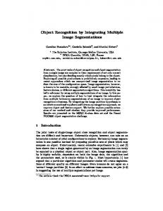
Figure 2-left shows a challenging example, which is used as case-study throughout the chapter. There is a large scale change (factor 3.3), out-of-plane rotation, extensive clutter and partial occlusion. All these factors make the life of the feature extraction and matching algorithms hard. A scheme of the approach is illustrated in figure 1. We build upon a multiscale extension of the extractor of [30]. However, the method works in conjunction with any affine invariant region extractor [1,13,15]. In the first phase (soft matching), we form a large set of initial region correspondences. The goal is to

148


obtain some correct matches also in difficult cases, even at the price of including a large majority of mismatches. Next, a grid of circular regions covering the model image is generated (coined coverage regions). The early expansion phase tries to propagate these coverage regions based on the geometric transformation of nearby initial matches. By propagating a region, we mean constructing the corresponding one in the test image. The propagated matches and the initial ones are then passed through a local filter, during the early contraction phase, which removes some of the mismatches. The processing continues by alternating faster expansion phases (main expansion), where coverage regions are propagated over a larger area, with contraction phases based on a global filter (main contraction). This filter exploits both topological arrangements and appearance information, and tolerates non-rigid deformations. The ‘early’ phases differ from the ‘main’ phases in that they are specialized to deal with the extremely low percentage of correct matches given by the initial matcher in particularly difficult cases.

model image test image

Soft matching

Early expansion

Early contraction

Main expansion

Main contraction

Fig. 1. Phases of the image exploration technique

3

Soft Matching

The first stage is to compute an initial set of region matches between a model image Im and a test image It . The region extraction algorithm [30] is applied to both images independently, producing two sets of regions Φm , Φt , and a vector of invariants describing each region [30]. Test regions Φt are matched to model regions Φm in two steps, explained in the next two subsections. The matching procedure allows for soft matches, i.e. more than one model region is matched to the same test region, or vice versa. 3.1

Tentative Matches

For each test region T ∈ Φt we first compute the Mahalanobis distance of the descriptors to all model regions M ∈ Φm . Next, the following appearance similarity measure is computed between T and each of the 10 closest model regions: dRGB(M, T ) ) (1) 100 where NCC is the normalized cross-correlation between the regions’ greylevel patterns, while dRGB is the average pixel-wise Euclidean distance in RGB colorspace after independent normalization of the 3 colorbands (necessary to achieve photometric invariance). Before computation, the two regions are aligned by the affine transformation mapping T to M . sim(M, T ) = NCC(M, T ) + (1 −


149

Fig. 2. Left: case-study, with model image (top), and test image (bottom). Middle: a close-up with 3 initial matches. The two model regions on the left are both matched to the same region in the test image. Note the small occluding rubber on the spoon. Righttop: the homogeneous coverage Ω. Right-bottom: a support region (dark), associated sectors (lines) and candidates (bright).

Each of the 3 test regions most similar to T above a low threshold t1 are considered tentatively matched to T . Repeating this operation for all regions T ∈ Φt , yields a first set of tentative matches. At this point, every test region could be matched to either none, 1, 2 or 3 model regions. 3.2

Refinement and Re-thresholding

Since all regions are independently extracted from the two images, the geometric registration of a correct match is often not optimal. Two matching regions often do not cover exactly the same physical surface, which lowers their similarity. The registration of the tentative matches is now refined using our algorithm [6], that efficiently looks for the affine transformation that maximizes the similarity. This results in adjusting the region’s location and shape in one of the images. Besides raising the similarity of correct matches, this improves the quality of the forthcoming expansion stage, where new matches are constructed based on the affine transformation of the initial ones. After refinement, the similarity is re-evaluated and only matches scoring above a second, higher threshold t2 are kept1 . Refinement tends to raise the similarity of correct matches much more than that of mismatches. The increased separation between the similarity distributions makes the second thresholding more effective. At this point, about 1/3 to 1/2 of the tentative matches are left. 1

The R, G, B colorbands range in [0, 255], so sim is within [−4.41, 2]. A value of 1.0 indicates good similarity. In all experiments the matching thresholds are t1 = 0.6, t2 = 1.0.

150

3.3


Motivation

The obtained set of matches usually still contains soft matches, i.e. more than one region in Φm is matched to the same region in Φt , or vice versa. This contrasts with previous works [1,12,15,18,30], but there are two good reasons for it. First, the scene might contain repeated, or visually similar elements. Secondly, large viewpoint and scale changes cause loss of resolution which results in a less accurate geometric correspondence and a lower similarity. When there is also extensive clutter, it might be impossible, based purely on local appearance [22], to decide which of the best 3 matches is correct, as several competing regions might appear very similar, and score higher than the correct match. A classic 1-to-1 approach may easily be distracted and fail to produce the correct match. The proposed process outputs a large set of plausible matches, all with a reasonably high similarity. The goal is to maximize the number of correct matches, even at the cost of accepting a substantial fraction of mismatches. This is important in difficult cases, when only a few model regions are re-extracted in the test image, because each correct match can start an expansion which will cover significant parts of the object. Figure 2-left shows the case-study, for which 3 correct matches out of 217 are found (a correct-ratio of 3/217). The large scale change, combined with the modest resolution (720x576), causes heavy image degradation which corrupts edges and texture. In such conditions only a few model regions are re-extracted in the test image and many mismatches are inevitable. In the rest of the chapter, we refer to the current set of matches as the configuration Γ . How to proceed ? Global, robust geometry filtering methods, like detecting outliers to the epipolar geometry through RANSAC [29] fail, as they need a minimal portion of inliers of about 1/3 [3,12]. Initially, this may very well not be the case. Even if we could separate out the few correct matches, they would probably not be sufficient to draw reliable conclusions about the presence of the object. In the following sections, we explain how to gradually increment the number of correct matches and simultaneously decrease the number of mismatches.

4

Early Expansion

4.1

Coverage of the Model Image

We generate a grid Ω of overlapping circular regions densely covering the model image Im (figure 2-top-right). In our implementation the grid is composed of a first layer of regions of radius 25 pixels, spaced 25 pixels, and a second layer with radius 13 pixels and spaced 25 pixels 2 . No regions are generated on the black background. According to various experiments, this choice of the parameters is not crucial for the overall recognition performance. The choice of the exact grid pattern, and consequently the number of regions in Ω, trades segmentation quality for computational cost, and could be selected based on the user’s desires. 2

These values are for an image of 720x576 pixels, and are proportionally adapted for images of other sizes.


151

At this point, none of the regions in Ω is matched to the test image It . The expansion phases will try to construct in It as many regions corresponding to them as possible. 4.2

Propagation Attempt

We now define the concept of propagation attempt which is the basic buildingblock of the expansion phases and will be used later. Consider a region Cm in model image Im without match in the test image It and a nearby region Sm , matched to St . If Cm and Sm lie on the same physical facet of the object, they will be mapped to It by similar affine transformations. The support match (Sm , St ) attempts to propagate the candidate region Cm to It as follows: 1. Compute the affine transformation A mapping Sm to St . 2. Project Cm to It via A : Ct = ACm . The benefits of exploiting previously established geometric transformations was also noted by [23]. 4.3

Early Expansion

Propagation attempts are used as a basis for the first expansion phase as follows. i Consider as supports {S i = (Sm , Sti )} the soft-matches configuration Γ , and as i candidates Λ the coverage regions Ω. For each support region Sm we partition i Im into 6 circular sectors centered on the center of Sm (figure 2-bottom-right). i attempts to propagate the closest candidate region in each sector. As Each Sm a consequence, each candidate Cm has an associated subset ΓCm ⊂ Γ of supports that will compete to propagate it. For a candidate Cm and each support S i in ΓCm do: 1. Generate Cti by attempting to propagate Cm via S i . 2. Refine Cti . If Cti correctly matches Cm , this adapts it to the local surface orientation (handles curved and deformable objects) and perspective effects (the affine approximation is only valid on a local scale). i i = {sR , sG , sB } between Sm and 3. Compute the color transformation TRGB i St . This is specified by the scale factors on the three colorbands. 4. Evaluate the quality of the refined propagation attempt, after applying the i color transformation TRGB i simi = sim(Cm , Cti , TRGB )= i Cm , Cti ) + (1 − NCC(TRGB

i dRGB(TRGB Cm ,Cti ) ) 100

i Applying TRGB allows to use the unnormalized similarity measure sim, because color changes are now compensated for. This provides more discriminative power over using sim.

152


We retain Ctbest , with best = arg maxi simi , the best refined propagation attempt. Cm is considered successfully propagated to Ctbest if simbest > t2 (the matching threshold). This procedure is applied for all candidates Cm ∈ Λ. Most support matches may actually be mismatches, and many of them typically lie around each of the few correct ones (e.g. several matches in a single soft-match, figure 2-middle). In order to cope with this situation, each support concentrates its efforts on the nearest candidate in each direction, as it has the highest chance to undergo a similar geometric transformation. Additionally, every propagation attempt is refined before evaluation. Refinement raises the similarity of correctly propagated matches much more than the similarity of mispropagated ones, thereby helping correct supports to win. This results in a limited, but controlled growth, maximizing the chance that each correct match propagates, and limiting the proliferation of mispropagations. The process also restricts the number of refinements to at most 6 per support (contains computational cost). For the case-study, 113 new matches are generated and added to the configuration Γ . 17 of them are correct and located around the initial 3 (figure 5, middle of top row). The correct-ratio of Γ improves to 20/330, but it is still very low.

5

Early Contraction

The early expansion guarantees good chances that each initial correct match propagates. As initial filter, we discard all matches that did not succeed in propagating any region. The correct-ratio of the case-study improves to 20/175 (no correct match is lost), but it is still too low for applying a global filter. Hence, we developed the following local filter. A local group of regions in the model image have uniform shape, are arranged on a grid and intersect each other with a specific pattern. If all these regions are correctly matched, the same regularities also appear in the test image, because the surface is contiguous and smooth (regions at depth discontinuities cannot be correctly matched anyway). This holds for curved or deformed objects as well, because the affine transformation varies slowly and smoothly across neighboring regions (figure 3-left). On the other hand, mismatches tend to be randomly located over the image and to have different shapes. i } be the neighbors We propose a local filter based on this observation. Let {Nm of a region Rm in the modelimage. Two regions A, B are considered neighbors if they intersect, i.e. if Area(A B) > 0. Only neighbors which are actually matched to the test image are considered. Any match (Rm , Rt ) is removed from Γ if i Area(Rm Nm Area(Rt Nti ) ) > ts − Area(Rm ) Area(Rt ) i

(2)

{Nm }

with ts some threshold3 . The filter, illustrated in figure 3-middle, tests the preservation of the pattern of intersections between R and its neighbors (the ratio of areas is affine invariant). Hence, a removal decision is based solely on local 3

This is set to 1.3 in all our experiments.

Simultaneous Object Recognition and Segmentation by Image Exploration Area(Rm

N m3 )

Nm3

Rm

Nm2

Nm1 Area(Rt

153

A N t3 )

Nt3

Rt

Nt1

Nt2

Fig. 3. Left: the pattern of intersection between neighboring correct region matches is preserved by transformations between the model and the test images, because the surface is contiguous and smooth. Middle: the surface contiguity filter evaluates this property by testing the conservation of the area ratios. Right: top: a candidate (thin) and 2 of 20 supports within the large circular area; bottom: the candidate is propagated to the test image using the affine transformation A of the support on the right (thick). Refinement adapts the shape to the perspective effects (brighter). The other support is mismatched to a region not visible in this close-up.

information. As a consequence, this filter is unaffected by the current, low overall ratio of correct matches. Shape information is integrated in the filter, making it capable of spotting insidious mismatches which are roughly correctly located, yet have a wrong shape. This is an advantage over the (semi-) local filter proposed by [24], and later also used by others [22,26], which verifies if a minimal amount of regions in an area around Rm in the model image also match near Rt in the test image. The input regions need not be arranged in a regular grid, the filter applies to a general set of (intersecting) regions. Note that isolated mismatches, which have no neighbors in the model image, will not be detected. The algorithm can be implemented to run in O((|Γ | + x) log(|Γ |)), with x |Γ |2 the number of region intersections [5, pp 202-203]. Applying this filter to the case-study brings the correct-ratio of Γ to 13/58, thereby greatly reducing the number of mismatches.

6

Main Expansion

The first early expansion and contraction phases brought several additional correct matches and removed many mismatches, especially those that concentrated around the correct ones. Since Γ is cleaner, we can now try a faster expansion.

154


All matches in the current configuration Γ are removed from the candidate i set Λ ← Λ\Γ , and are used as supports. All support regions Sm in a circular 4 area around a candidate Cm compete to propagate it: 1. Generate Cti by attempting to propagate Cm via S i . i 2. Compute the color transformation TRGB of S i . i i 3. Evaluate simi = sim(Cm , Ct , TRGB ). We retain Ctbest , with best = arg maxi simi and refine it, yielding Ctref . Cm is considered successfully propagated to Ctref if sim(Cm , Ctref ) > t2 (figure 3-right). This scheme is applied for each candidate. In contrast to the early expansion, many more supports compete for the same candidate, and no refinement is applied before choosing the winner. However, the presence of more correct supports, now tending to be grouped, and fewer mismatches, typically spread out, provides good chances that a correct support will win a competition. In this process each support has the chance to propagate many more candidates, spread over a larger area, because it offers help to all candidates within a wide circular radius. This allows the system to grow a mass of correct matches. Moreover, the process can jump over small occlusions or degraded areas, and costs only one refinement per candidate. For the case-study, 185 new matches, 61 correct, are produced, thus lifting the correct-ratio of Γ up to 74/243 (31%, figure 5, second row).

7

Main Contraction

At this point the chances of having a sufficient number of correct matches for applying a global filter are much better. We propose here a global filter based on a topological constraint for triples of region matches. In contrast to the local filter of section 5, this filter is capable of finding also isolated mismatches. The next subsection introduces the constraint on which the filter is based, while the following two subsections explain the filter itself and discuss its qualities. 7.1

The Sidedness Constraint

1 2 3 , Rm , Rm ) of regions in the model image and their matching Consider a triple (Rm 1 2 3 regions (Rt , Rt , Rt ) in the test image. Let cjv be the center of region Rvj (v ∈ {m, t}). The function

side(Rv1 , Rv2 , Rv3 ) = sign((c2v × c3v )c1v )

(3)

takes value −1 if c1v is on the right side of the directed line c2v × c3v , going from c2v to c3v , or value 1 if it’s on the left side. The equation 1 2 3 , Rm , Rm ) = side(Rt1 , Rt2 , Rt3 ) side(Rm 4

In all experiments the radius is set to 1/6 of the image size.

(4)


155

states that c1 should be on the same side of the line in both views (figure 4left). This sidedness constraint holds for all correctly matched triples of coplanar regions, because in this case property (3) is viewpoint invariant. The constraint is valid also for most non-coplanar triples. A triple violates the constraint if at least one of the three regions is mismatched, or if they are not coplanar and there is important camera translation in the direction perpendicular to the 3D plane containing their centers (parallax-violation). This can create a parallax effect strong enough to move c1 to the other side of the line. Nevertheless, this phenomenon typically affects only a small minority of triples. Since the camera can only translate in one direction between two views, the resulting parallax can only corrupt few triples, because those on planes oriented differently will not be affected. The region matches violate or respect equation (4) independently of the order in which they appear in the triple. The three points should be cyclically ordered in the same orientation (clockwise or anti-clockwise) in the two images in order to satisfy (4). Topological configurations of points and lines were also used by Tell and Carlsson [28] in the wide-baseline stereo context, as a mean for guiding the matching process. 7.2

Topological Filter

A triple including a mismatched region has higher chances to violate the sidedness constraint. When this happens, it indicates that probably at least one of the matches is incorrect, but it does not tell which one(s). While one triple is not enough to decide, this information can be recovered by considering all triples simultaneously. By integrating the weak information each triple provides, it is possible to robustly discover mismatches. The key idea is that we expect incorrectly located regions to be involved in a higher share of violations. The constraint is checked for all unordered triples (Ri , Rj , Rk ), Ri , Rj , Rk ∈ Γ . The share of violations for a region match Ri is errtopo (Ri ) =

1 v

i j k |side(Rm , Rm , Rm ) − side(Rti , Rtj , Rtk )|

(5)

Rj ,Rk ∈Γ \Ri ,j>k

with v = (n − 1)(n − 2)/2, n = |Γ |. errtopo (Ri ) ∈ [0, 1] because it is normalized w.r.t. the maximum number of violations v any region can be involved in. The topological error share (5) is combined with an appearance term, giving the total error i errtot (Ri ) = errtopo(Ri ) + (t2 − sim(Rm , Rti ))

The filtering algorithm starts from the current set of matches Γ , and then iteratively removes one match at a time as follows: 1. (Re-)compute errtot (Ri ) for all Ri ∈ Γ . 2. Find the worst match Rw , with w = arg maxi errtot (Ri )

156


3. If errtot (Rw ) > 0, remove Rw from Γ . Rw will not be used for the computation of errtopo in the next iteration. Iterate to 1. If errtot (Rw ) ≤ 0, or if all matches have been removed, then stop.

D

c 1m

2 cm

C

c 3m c2t c 1t

c 3t

A

B

C D

B

A

Fig. 4. Sidedness constraints. Left: c1 should be on the same side of the directed line from c2 to c3 in both images. Right: the constraints hold also for deformed objects. The small arrows indicate ’to the right’ of the directed lines A → B, B → C, C → D, D → A.

At each iteration the most probable mismatch Rw is removed. During the first iterations many mismatches might still be present. Therefore, even correct matches might have a moderately large error, as they take part in triples including mismatches. However, mismatches are likely to have an even larger error, because they are involved in the very same triples, plus other violating ones. Hence, the worst mismatch Rw , the region located in It farthest from where it should be, is expected to have the largest error. After removing Rw all errors decrease, including the errors of correct matches, because they are involved in less triples containing a mismatch. After several iterations, ideally only correct matches are left. Since these have only a low error, due to occasional parallax-violations, the algorithm stops. The second term of errtot decreases with increasing appearance similarity, i , Rti ) = t2 , the matches acceptance threshold. The and it vanishes when sim(Rm removal criterion errtot > 0 expresses the idea that topological violations are accepted up to the degree to which they are compensated by high similarity. This helps finding mismatches which can hardly be judged by only one cue. A typical mismatch with similarity just above t2 , will be removed unless it is perfectly topologically located. Conversely, correct matches with errtopo > 0 due to parallax-violations are in little danger, because they typically have good


157

similarity. Including appearance makes the filter more robust to low correctratios, and remedies the potential drawback (parallax-violations) of a purely topological filter [6]. In order to achieve good computational performance, we store the terms of the sum in function (5) during the first iteration. In the following iterations, the sum is quickly recomputed by retrieving and adding up the necessary terms. This makes the computational cost almost independent of the number of iterations. The algorithm can be implemented to run in O(n2 log(n)), based on the idea of constructing, for each point, a list with a cyclic ordering of all other points (a complete explanation is given in [5, pp. 208-211]). 7.3

Properties and Advantages

The proposed filter has various attractive properties, and offers several advantages over detecting outliers to the epipolar geometry through RANSAC [29], which is traditionally used in the matching literature [13,15,22,23,30]. In the following, we refer to it as RANSAC-EG. The main two advantages are (more discussion in [5, pp. 75-77]): It allows for non-rigid deformations. The filter allows for non-rigid deformations, like the bending of paper of cloth, because the structure of the spatial arrangements, captured by the sidedness constraints, is stable under these transformations. As figure 4-right shows, sidedness constraints are still respected even in the presence of substantial deformations. Other filters, which measure a geometrical distance error from an estimated model (e.g. homography, fundamental matrix) would fail in this situation. In the best case, several correct matches would be lost. Worse yet, in many cases the deformations would disturb the estimation of the model parameters, resulting in a largely random behavior. The proposed filter does not try to capture the transformations of all matches in a single, overall model, but it relies instead on simpler, weak properties, involving only three matches each. The discriminative power is then obtained by integrating over all measurements, revealing their strong, collective information. It is insensitive to inaccurate locations. The regions’ centers need not be exactly localized, because errtopo varies slowly and smoothly for a region departing from its ideal location. Hence, the algorithm is not affected by perturbations of the region’s locations. This is precious in the presence of large scale changes, not completely planar regions, or with all kinds of image degradation (motion blur, etc.), where localization errors become more important. In RANSAC-EG instead, the point must lie within a tight band around the epipolar line. Worse yet, inaccurate localization of some regions might compromise the quality of the fundamental matrix, and therefore even cause rejection of many accurate regions [33]. In [5, pp. 84-85] we report experiments supporting this point, where the topological filter could withstand large random shifts on the regions’ locations (about 25 pixels, in a 720x576 image).

158


7.4

Main Contraction on the Case-Study

After main expansion, the correct-ratio of the case-study was of 74/243. Applying the filter presented in this section brings it to 54/74, which is a major improvement (figure 5 second row). 20 correct matches are lost, but many more mismatches are removed (149). The further processing will recover the correct matches lost and generate even more.

8

Exploring the Test Image

The processing continues by iteratively alternating main expansion and main contraction phases. 1. Do a main expansion phase. All current matches Γ are used as supports. This produces a set of propagated region matches Υ , which are added to the configuration: Γ ← (Γ Υ ). 2. Do a main contraction phase on Γ . This removes matches from Γ . 3. If at least one newly propagated region survives the contraction, i.e. if |Υ Γ | > 0, then iterate to point 1, after updating the candidate set to contain Λ ← (Ω\Γ ), all original candidate regions Ω which are not yet in the configuration. Stop if no newly propagated regions survived, or if all regions Ω have been propagated. In the first iteration, the expansion phase generates some correct matches, along with some mismatches. Because a correct match tends to propagate more than a mismatch, the correct ratio increases. The first main contraction phase removes mostly mismatches, but might also lose several correct matches: the amount of noise (percentage of mismatches) could still be high and limit the filter’s performance. In the next iteration, this cleaner configuration is fed into the expansion phase again which, less distracted, generates more correct matches and fewer mismatches. The new correct matches in turn help the next contraction stage in taking better removal decisions, and so on. As a result, the number, percentage and spatial extent of correct matches increase at every iteration, reinforcing the confidence about the object’s presence and location (figure 6). The two goals of separating correct matches and gathering more information about the object are achieved at the same time. Correct matches erroneously killed by the contraction step in an iteration get another chance during the next expansion phase. With even fewer mismatches present, they are probably regenerated, and this time have higher chances to survive the contraction (higher correct-ratio, more positive evidence present). Thanks to the refinement, each expansion phase adapts the shape of the newly created regions to the local surface orientation. Thus the whole exploration process follows curved surfaces and deformations. The exploration procedure tends to ‘implode’ when the object is not in the test image, typically returning only a few matches. Conversely, when the object is present, the approach fills the visible portion of the object with many high


soft matching 3/217

first main expansion 74/243

second main contraction 150/174

early expansion 20/330

first main contraction 54/74

159

early contraction 13/58

second main expansion 171/215

contours of the final set of matches

Fig. 5. Evolution of Γ for the case-study. Top rows: correct matches; bottom rows: mismatches.

160

V. Ferrari, T. Tuytelaars, and L. Van Gool 250 second main expansion

200 150 100 50

early expansion

soft matches

first main expansion

final

second main contraction

first main contraction

early contraction remove non−propagating

Fig. 6. The number of correct matches for the case-study increases at every iteration (compare the points after each contraction phase)

confidence matches. This yields high discriminative power and the qualitative shift from only detecting the object to knowing its extent in the image and which parts are occluded. Recognition and segmentation are two aspects of the same process. In the case-study, the second main expansion propagates 141 matches, 117 correct, which is better than the previous 61/185. The second main contraction starts from 171/215 and returns 150/174, killing a lower percentage of correct matches than in the first iteration. After the 11th iteration 220 matches cover the whole visible part of the object (202 are correct). Figure 5 depicts the evolution of the set of matches Γ . The correct matches gradually cover more and more of the object, while mismatches decrease in number. The system reversed the situation, by going from only very few correct matches in a large majority of mismatches, to hundreds of correct matches with only a few mismatches. Notice the accuracy of the final segmentation, and in particular how the small occluding rubber has been correctly left out (figure 5 bottom-right).

9

Results

9.1

Recognition from Still Images

The dataset in this subsection5 consists of 9 model objects and 23 test images. In total, the objects appear 43 times, as some test images contain several objects. To facilitate the discussion, the images are referred to by their coordinates as in figure 7, where the arrangement is chosen so that a test image is adjacent to the model object(s) it contains. There are 3 planar objects, each modeled by a single view, including a Kellogs box6 and two magazines, Michelle (figure c2) and Blonde (analog model view). Two objects with curved shapes, Xmas (b1) and Ovo (e2), have 6 model views. Leo (d3), Car (a2), Suchard (d1) feature more complex 3D shapes and have 8 model views. Finally, one frontal view models the last 3D object, Guard (b3). Multiple model views are taken equally spaced around the object. The contributions from all model views of a single object are combined by superimposing the area covered by the final set of matched regions (to find the contour), and by summing their number (detection criterion). 5 6

The dataset is available at www.vision.ee.ethz.ch/∼ferrari. The kellogs box is used throughout the chapter as a case-study.


1

2

a

b

c

d

e

Fig. 7. Recognition results (see text)

3

161

162


All images are shot at a modest resolution (720x576) and all experiments are conducted with the same set of parameters. In general, in the test cases there is considerable clutter and the objects appear smaller than in the models (all model images have the same resolution as the test images and they are shown at the same size). Tolerance to non-rigid deformations is shown in c1, where Michelle is simultaneously strongly folded and occluded. The contours are found with a good accuracy, extending to the left until the edge of the object. Note the extensive clutter. High robustness to viewpoint changes is demonstrated in c3, where Leo is only half visible and captured in a considerably different pose than any of the model views, while Michelle undergoes a very large out-of-plane rotation of about 80 degrees. Guard, occluding Michelle, is also detected in the image, despite a scale change of factor 3. In d2, Leo and Ovo exhibit significant viewpoint changes, while Suchard is simultaneously scaled by factor 2.2 and 89% occluded. This very high occlusion level makes this case challenging even for a human observer. A scale change of factor 4 affecting Suchard is illustrated in e1. In figure a1, Xmas is divided in two by a large occluder. Both visible parts are correctly detected by the presented method. On the right side of the image, Car is found even if half occluded and very small. Car is also detected in spite of a considerable viewpoint change in a3. The combined effects of strong occlusion, scale change and clutter make b2 an interesting case. Note how the boundaries of Xmas are accurately found, and in particular the detection of the part behind the glass. As a final example, 8 objects are detected at the same time in e3 (for clarity, only 3 contours are shown). Note the correct segmentation of the two deformed magazines and the simultaneous presence of all the aforementioned difficulties. Figure 8-bottom-left presents a close-up on one of 93 matches produced between a model view of Xmas (left) and test case b2 (right). This exemplifies the great appearance variation resulting from combined viewpoint, scale and illumination changes, and other sources of image degradation (here a glass). In these cases, it is very unlikely for the region to be detected by the initial region extractor, and hence traditional methods fail. As a proof of the method’s capability to follow deformations, we processed the case in figure 8-bottom-right starting with only one match (dark). 356 regions, covering the whole object, were produced. Each region’s shape fits the local surface orientation (for clarity, only 3 regions are shown). The performance of the system was quantified by processing all pairs of modelobject and test images, and counting the resulting number of region matches. The highest ROC curve in figure 8-top-left depicts the detection rate versus false-positive rate, while varying the detection threshold from 0 to 200 matches. An object is detected if the number of produced matches, summed over all its model views, exceeds this threshold. The method performs very well, and can achieve 98% detection with 6% false-positives. For comparison, we processed the dataset also with 4 state-of-the-art affine region extractors [1,15,18,30], and

Simultaneous Object Recognition and Segmentation by Image Exploration this paper

Legend MS02

TVG00

TVG00 org

OM02

Bau00

MS02 Mikolajczyk and Schmid 2002

163

percentage of cases

percentage of cases

OM02 Obrdzalek and Matas 2002 30%

30%

Bau00 Baumberg 2000 TVG000 Tuytelaars and Van Gool 2000

200

number of matches (score)

30

number of matches (score)

Fig. 8. Top: left: ROC plot. False-positives on the X-axis, detection rate on the Y-axis; middle: distribution of scores for our method (percentage; bright = positive cases; dark = negative cases); right: for the traditional matching of the regions of Matas et al. Bottom: left: close-up on one match of case b2; right: starting from the black region only, the method covers the magazine with 365 regions (3 shown).

described the regions with the SIFT [12] descriptor7 , which has recently been demonstrated to perform best [4]. The matching is carried out by the ’unambiguous nearest-neighbor’ approach8 advocated in [1,12]: a model region is matched to the region of the test image with the closest descriptor if it is closer than 0.7 times the distance to the second-closest descriptor (the threshold 0.7 has been empirically determined to optimize results). Each of the central curves illustrates the behavior of a different extractor. As can be seen, none is satisfactory, which demonstrates the higher level of challenge posed by the dataset and therefore suggests that our approach can broaden the range of solvable object recognition cases. Closer inspection reveals the source of failure: typically only very few, if any, correct matches are produced when the object is present, which in turn is due to the lack of repeatability and the inadequacy of a simple matcher under such difficult conditions. The important improvement brought by the proposed method is best quantified by the difference between the highest curve and the central thick curve, representing the system we started from [30] (’TVG00 org’ in the plot). 7

8

All region extractors and the SIFT descriptor are implementations of the respective authors. We are grateful to J. Matas, K. Mikolajczyk, A. Zisserman, C. Schmid and D. Lowe. We have also tried the standard approach, used in [15,4,18,30], which simply matches two nearest-neighbors if their distance is below a threshold, but it produced slightly worse results.

164


Figure 8-top-middle shows a histogram of the number of final matches (recognition score) output by our system. The scores assigned when the object is in the test image (positive cases) are much higher than when the object is absent (negative cases), resulting in very good discriminative power. As a comparison with the traditional methods, the standard matching of regions of [18], based on the SIFT descriptor, yields two hardly separable distributions (figure 8-top-right), and hence the unsatisfactory performance in the ROC plot. Similar histograms are produced based on the other feature extractors [1,15,30]. 1

2

3

4

a

b

c

Fig. 9. Video retrieval results. The parts of the model-images not delineated by the user are blanked out.

As last comparison, we consider the recent system [21], which constructs a 3D model of each object prior to recognition. We asked the authors to process our dataset. As they reported, because of the low number of model views, their system couldn’t produce meaningful models, and therefore couldn’t perform recognition. Conversely, we have processed the dataset of [21] with our complete system (including multi-view integration [7]). It performed well, and achieved 95% detection rate for 6% false-positives (see [21] for more details). 9.2

Video Retrieval

In this experiment, the goal is to find a specific object or scene in a test video. The object is only given as delineated by the user in one model image. In [26]


165

another region-based system for video object retrieval is presented. However, it focuses on different aspects of the problem, namely the organization of regions coming from several shots, and weighting their individual relevance in the wider context of the video. At the feature level, their work still relies solely on regions from standard extractors. Because of the different nature of the data, the system differs in a few points from the object recognition one. At recognition time the test video is segmented into shots, and a few representative keyframes are selected in each shot by the algorithm of [19]. The object is then searched in each keyframe separately, by a simplified version of the image exploration technique. Specifically, it has a simple one-to-one nearest neighbor approach for the initial matching instead of the soft-matching phase, there are no ‘early’ phases, and there is only one layer of coverage regions. This simpler version runs faster (about twice as fast), though it is not as powerful. It takes about 2 minutes to process a (object,keyframe) pair on a common workstation (2.4 Ghz PC). We present results on challenging, real-world video material, namely news broadcast provided by the RTBF Belgian television. The data comes from 4 videos, captured on different days, each of about 20 minutes. The keyframes have low resolution (672x528) and many of them are visibly affected by compression artifacts, motion blur and interlacing effects. We selected 13 diverse objects, including locations, advertising products, logos and football shirts, and delineated each in one keyframe. Each object is searched in the keyframes of the video containing its model-image. On average, a video has 325 keyframes, and an object occurs 7.4 times. The number of keyframes not containing an object (negatives), is therefore much greater than the number of positives, allowing to collect relevant statistics. A total of 4236 (object,keyframe) image pairs have been processed. Figure 9.1 show some example detections. A large piece of quilt decorated with various flags (a2) is found in a3 in spite of non-rigid deformation, occlusion and extensive clutter. An interesting application is depicted in b1-b2-b3. The shirts of two football teams are picked out as query objects (b2), and the system is asked to find the keyframes where each team is playing. In b1 the Fortis shirt is successfully found in spite of important motion blur (close-up in a1). Both teams are identified in b3, where the shirts appear much smaller and the Dexia player is turned 45 degrees (viewpoint change on the shirt). The keyframe in c1 instead, has not been detected. Due to the intense blur, the initial matcher does not return any correct correspondence. Robustness to large scale changes and occlusion is demonstrated in a4, where the UN council, modeled in b4, is recognized while enlarged by a scale factor 2.7, and heavily occluded (only 10% visible). Equally intriguing is the image of figure c4, where the UN council is seen from an opposite viewpoint. The large painting on the left of b4 is about the only thing still visible in the test keyframe, where it appears on the right side. The system matched the whole area of the painting, which suffers from out-of-plane rotation. As a last example, a room with Saddam Hussein is found

166


in figure c3 (model in c2). The keyframe is taken under a different viewpoint and substantially corrupted by motion blur. The retrieval performance is quantified by the detection rate and false-positive rate, averaged over all objects. An object is detected if the number of final matches, divided by the number of model coverage regions, exceeds 10% (detections of model-keyframes are not counted). The system performs well, by achieving an average detection rate of 82.4%, for a false-positive rate of 3.6%. As a comparison, we repeated the experiment with [30], the method we started from. It only managed a 33.3% detection rate, for a false-positive rate of 4.6%, showing that our approach can substantially boost the performance of standard affine invariant matching procedures.

10

Related Work

The presented technique belongs to the category of appearance-based object recognition. Since it can extend any approach which matches affine invariant regions between images, it is tightly related to this class of methods. The novelties and improvements brought by our approach are enumerated in the introduction section and demonstrated in the result section 9. Beyond the realm of local invariant features, there are a few works which are related to ours, in that they also combine recognition with segmentation. Leibe and Schiele [10] present a method to detect an unknown object instance of a given category and segment it from a test image. The category (e.g. cows) is learnt from example instances (images of particular cows). However, the method does not support changes in camera viewpoint or orientation. In [32], low-level grouping cues based on edge responses, high-level cues from a part detector and spatial consistency of detected parts, are combined in a graph partitioning framework. The scheme is shown to recognize and segment a human body in a cluttered image. However, the part detectors need a considerable number of training examples, and the very parts to be learned are manually indicated (head, left arm, etc.). Moreover, there is no viewpoint, orientation or scale invariance. Both methods are suited for categorization, and not specialized in the recognition of a particular objects. While we believe our approach to be essentially original, some components are clearly related to earlier research. The filter in section 7 is constructed around the sidedness constraint. A similar constraint, testing the cyclic ordering of points, was used for wide-baseline matching in [28]. Moreover, the ‘propagation attempt’ at the heart of the expansion phases is an evolution of the idea of ‘growing matches’ proposed by [20,23,22]. While they use existing affine transformations only to guide the search for further matches, our approach actively generates new regions, which have not been originally extracted. This is crucial to counter the repeatability problems stated in the introduction. Finally, a different, pixel-bypixel propagation strategy was previously proposed in [11], but it is applicable only in case of small differences between the images.


11

167

Conclusion and Outlook

We have presented an approach to object recognition capable of solving particularly challenging cases. Its power roots in the ‘image exploration’ technique. Every single correct match can lead to the generation of many correct matches covering the smooth surface on which it lies, even when starting from an overwhelming majority of mismatches. Hence, the method can boost the performance of any algorithm which provides affine regions correspondences, because very few correct initial matches suffice for reliable recognition. Moreover, the approximate boundaries of the object are found during the recognition process, and non-rigid deformations are explicitly taken into account, two features lacking in competing approaches (e.g. [1,12,15,18,21,22,30]). Some individual components of the scheme, like the topological filter and GAMs, are useful in their own right, and can be used profitably beyond the scope of this chapter. In spite of the positive points expressed above, our approach is not without limitations. One of them is the computational expense: in the current implementation, a 2.4 Ghz computer takes about 4-5 minutes, on average, to process a pair of model and test images. Although we plan a number of speedups, the method is unlikely to reach the speed of the fastest other systems (the system of Lowe [12] is reported to perform recognition within seconds). As another limitation, our method is best suited for objects which have some texture, much like the other recognition schemes based on invariant regions. Uniform objects (e.g. a balloon) cannot be dealt with and seem out of the reach of this kind of approaches. They should be addressed by techniques based on contours [4,25]. Hence, a useful extension would be to combine some sort of ‘local edge regions’ with the current textured regions. An important evolution is the systematic exploitation of the relationships between multiple overlapping model views. We have tackled this issue in a separate publication [7]. Finally, using several types of affine invariant regions simultaneously, rather than only those of [30], would push the performance further upwards.

References 1. A. Baumberg. Reliable feature matching across widely separated views. In Proceedings of the International Conference on Computer Vision, pages 774–781, 2000. 2. G. Bebis, M. Georgiopoulos, and N. V. Lobo. Learning geometric hashing functions for model-based object recognition. In Proceedings of the International Conference on Computer Vision, pages 543–548, 1995. 3. O. Chum, J. Matas, and S. Obdrzalek. Epipolar geometry from three correspondences. In Proceedings of Computer Vision Winter Workshop, 2003. 4. C. Cyr and B. Kimia. 3d object recognition using similarity-based aspect graph. In Proceedings of the International Conference on Computer Vision, 2001. 5. V. Ferrari. Affine Invariant Regions ++. PhD Thesis, Selected Readings in Vision and Graphics, Springer Verlag, Zuerich, CH, 2004.

168


6. V. Ferrari, T. Tuytelaars, and L. Van-Gool. Wide-baseline multiple-view correspondences. In Proceedings of the IEEE Conference on Computer Vision and Pattern Recognition, 2003. 7. V. Ferrari, T. Tuytelaars, and L. Van-Gool. Integrating multiple model views for object recognition. In Proceedings of the IEEE Conference on Computer Vision and Pattern Recognition, 2004. 8. V. Ferrari, T. Tuytelaars, and L. Van-Gool. Simultaneous object recognition and segmentation by image exploration. In Proceedings of the European Conference on Computer Vision, 2004. 9. V. Ferrari, T. Tuytelaars, and L. Van-Gool. Simultaneous object recognition and segmentation from single or multiple model views. to appear in International Journal of Computer Vision, 2006. 10. B. Leibe and B. Schiele. Scale-invariant object categorization using a scale-adaptive mean-shift search. In Proceedings of DAGM, pages 145–153, 2004. 11. M. Lhuillier and L. Quan. Match propagation for image-based modeling and rendering. IEEE Transactions on Pattern Analysis and Machine Intelligence, 24(12), 2002. 12. D. Lowe. Distinctive image features from scale-invariant keypoints. to appear in International Journal of Computer Vision, 2004. 13. J. Matas, O. Chum, M. Urban, and T. Pajdla. Robust wide baseline stereo from maximally stable extremal regions. In Proceedings of the British Machine Vision Conference, 2002. 14. K. Mikolajczyk and C. Schmid. Indexing based on scale-invariant interest points. In Proceedings of the International Conference on Computer Vision, 2001. 15. K. Mikolajczyk and C. Schmid. An affine invariant interest point detector. In Proceedings of the European Conference on Computer Vision, 2002. 16. K. Mikolajczyk and C. Schmid. A performance evaluation of local descriptors. In Proceedings of the IEEE Conference on Computer Vision and Pattern Recognition, volume II, pages 257–263, 2003. 17. H. Murase and S. Nayar. Visual learning and recognition of 3d objects from appearance. International Journal of Computer Vision, 14(1), 1995. 18. S. Obrdzalek and J. Matas. Object recognition using local affine frames on distinguished regions. In Proceedings of the British Machine Vision Conference, pages 414–431, 2002. 19. M. Osian and L. Van-Gool. Video shot characterization. In Proceedings of the TRECVID Workshop, 2003. 20. P. Pritchett and A. Zisserman. Wide baseline stereo matching. In Proceedings of the IEEE Conference on Computer Vision and Pattern Recognition, 1998. 21. F. Rothganger, S. Lazebnik, C. Schmid, and J. Ponce. 3d object modeling and recognition using affine-invariant image descriptors and multi-view spatial constraints. to appear in International Journal of Computer Vision, 2005. 22. F. Schaffalitzky and A. Zisserman. Automated scene matching in movies. In Proceedings of the Workshop on Content-based Image and Video Retrieval, 2002. 23. F. Schaffalitzky and A. Zisserman. Multi-view matching for unordered image sets. In Proceedings of the European Conference on Computer Vision, 2002. 24. C. Schmid. Combining greyvalue invariants with local constraints for object recognition. In Proceedings of the IEEE Conference on Computer Vision and Pattern Recognition, pages 872–877, 1996. 25. A. Selinger and R. C. Nelson. A perceptual grouping hierarchy for appearancebased 3d object recognition. Computer Vision and Image Understanding, 76(1):83– 92, 1999.


169

26. J. Sivic and A. Zisserman. Video google: A text retrieval approach to object matching in videos. In Proceedings of the International Conference on Computer Vision, 2003. 27. M. J. Swain and B. H. Ballard. Color indexing. International Journal of Computer Vision, 7(1):11–32, 1991. 28. D. Tell and S. Carlsson. Combining appearance and topology for wide baseline matching. In Proceedings of the European Conference on Computer Vision, pages 68–81, 2002. 29. P.H.S. Torr and D. W. Murray. The development and comparison of robust methods for estimating the fundamental matrix. International Journal of Computer Vision, 24(3):271–300, 1997. 30. T. Tuytelaars and L. Van-Gool. Wide baseline stereo based on local, affinely invariant regions. In Proceedings of the British Machine Vision Conference, 2000. 31. T. Tuytelaars, L. Van-Gool, L. Dhaene, and R. Koch. Matching affinely invariant regions for visual servoing. In Proceedings of the IEEE Conference on Robotics and Automation, pages 1601–1606, 1999. 32. S. X. Yu, R. Gross, and J. Shi. Concurrent object recognition and segmentation by graph partitioning. In Neural Information Processing Systems, 2002. 33. Z. Zhang, R. Deriche, O. Faugeras, and Q. Luong. A robust technique for matching two uncalibrated images through the recovery of the unknown epipolar geometry. Artificial Intelligence, 78:87–119, 1995.