Hindawi Publishing Corporation BioMed Research International Volume 2015, Article ID 454765, 21 pages http://dx.doi.org/10.1155/2015/454765
Research Article Simultaneous Parameters Identifiability and Estimation of an E. coli Metabolic Network Model Kese Pontes Freitas Alberton,1 André Luís Alberton,2 Jimena Andrea Di Maggio,3 Vanina Gisela Estrada,3 María Soledad Díaz,3 and Argimiro Resende Secchi1 1
Programa de Engenharia Qu´ımica-COPPE, Universidade Federal do Rio de Janeiro, Cidade Universit´aria, 21941-972 Rio de Janeiro, BR, Brazil 2 Instituto de Qu´ımica, Universidade do Estado do Rio de Janeiro, S˜ao Francisco Xavier 524, 20550-900 Rio de Janeiro, BR, Brazil 3 Planta Piloto de Ingenier´ıa Qu´ımica-CONICET, Universidad Nacional del Sur, Camino La Carrindanga, Km 7, 8000 Bah´ıa Blanca, Argentina Correspondence should be addressed to Kese Pontes Freitas Alberton;
[email protected] Received 31 May 2014; Revised 29 August 2014; Accepted 5 September 2014 Academic Editor: Eug´enio Ferreira Copyright © 2015 Kese Pontes Freitas Alberton et al. This is an open access article distributed under the Creative Commons Attribution License, which permits unrestricted use, distribution, and reproduction in any medium, provided the original work is properly cited. This work proposes a procedure for simultaneous parameters identifiability and estimation in metabolic networks in order to overcome difficulties associated with lack of experimental data and large number of parameters, a common scenario in the modeling of such systems. As case study, the complex real problem of parameters identifiability of the Escherichia coli K-12 W3110 dynamic model was investigated, composed by 18 differential ordinary equations and 35 kinetic rates, containing 125 parameters. With the procedure, model fit was improved for most of the measured metabolites, achieving 58 parameters estimated, including 5 unknown initial conditions. The results indicate that simultaneous parameters identifiability and estimation approach in metabolic networks is appealing, since model fit to the most of measured metabolites was possible even when important measures of intracellular metabolites and good initial estimates of parameters are not available.
1. Introduction The development of mathematical model for metabolic networks has been severely hampered by the lack of kinetic information [1–4]. Usually, available experimental data are obtained under different conditions using heterogeneous techniques, whose choice must be done according to the observation of a specific phenomenon of interest on the pathways [2, 4–6]. In such systems, the type of experiment, sampling method, and the mathematical interpretation of the data depend on the desired experimental information [5]. However, as pointed out by Costa et al. [4], kinetic information presented in the literature about metabolic network models is scarce and often confuse; thus, other strategies are adopted in detriment to the dynamic simulation of such systems.
Mathematically, metabolic networks are described by complex dynamics models, whose structure is composed by ordinary differential equations that represent mass balance of the substrate, biomass, products and intracellular metabolites crucial on the pathways, and numerous reaction rates regarding to the pathways. Such mathematical structure presents a large number of parameters, for which the estimation procedure demands a considerable number of experimental data. Since experimentally metabolic networks are only partially observed, only a fraction of the intracellular metabolites considered in the mathematical model can be directly measured and thus initial conditions should also be estimated. Unfortunately, in metabolic network systems, lack of experimental data is almost unavoidable, which compromises the reliability of reactions rates proposition and makes the estimation of all parameters unfeasible. Thus, such
2 problems often require the use of parameters identifiability procedures. Parameters identifiability procedures deal with ill-posed parameters estimation problems, selecting a subset of parameters that can be estimated when the estimation of all parameters is not possible [7]. In most procedures, parameters are ranked from most estimable to least estimable based on the structure of the model, the experimental measurements and their uncertainties, and the uncertainties of the initial estimates [8]. Several studies reported in the literature addressing the parameters identifiability in metabolic networks are exclusively concentrated in the model structure, called structural identifiability (e.g., Davidescu and Jørgensen [9]; Roper et al. [10]; Nikerel et al. [11]), and do not take into account the available experimental data. On other side, the practical identifiability (e.g., Srinath and Gunawan [12]) investigates if the available experimental data are appropriate and sufficient for achieving a reliably estimation of the model parameters. Although the structural identifiability is a necessary condition, the practical identifiability must overcome additional difficulties, including the selection of parameters with low sensitivity on the model predictions and correlation among parameters [13]. Unfortunately, such analyses in complex models depend on the values of parameters [13], generally unavailable [8]. Since sensitivity analysis is a key tool of identifiability procedures, procedures that evaluate the identifiability only based on initial parameters values can lead to a subset of selected parameters whose estimation may lead to an illposed problem [7]. A strategy to soften this problem is to perform simultaneous parameters selection and estimation, which ensures the estimation of the selected parameters (e.g., Secchi et al. [14], Wu et al. [15]; Wu et al. [16]; McLean et al. [17]; Alberton et al. [18]). Several procedures adopt as stop criterion the singularity of FIM (Fisher Information Matrix) (e.g., Weijers and Vanrolleghem [19]; Sandink et al. [20]; Li et al. [21]; Secchi et al. [14]; Lund and Foss [22]; Thompson et al. [8]; Alberton et al. [18]). The singularity of the FIM matrix, calculated only with the selected parameters, indicates the point in which estimation problem becomes ill-posed. When such point is reached, the parameters selection is stopped and the remaining parameters are admitted as nonidentifiable parameters. Particularly when identifiability performs simultaneous parameters selection and estimation (e.g., Secchi et al. [14]; Wu et al. [15]; Wu et al. [16]; McLean et al. [17]; Alberton et al. [18]), it is not desirable to keep the remaining parameters as nonidentifiable without evaluation of their estimation potential, because the estimation problem is modified at each selected parameter. A great challenge to be overcame in identifiability procedures, even those which include simultaneous estimation, is that the nonselected parameters are evaluated based on their initial estimates, which are probably inadequate. The literature addresses Monte Carlo techniques [23] and simultaneous parameters reestimation for assuring well posed estimation of the selected parameters (e.g., Secchi et al. [14], Wu et al. [15]; Wu et al. [16]; McLean et al. [17]; Alberton et al. [18]).
BioMed Research International As more proper, the evaluation of subsequent parameters to be selected should be done based on the reestimated selected parameters values [17, 18], reducing the dependence on the initial parameters estimates. In an interesting work, McLean et al. [17] developed an algorithm which allows evaluating the identifiability of all parameters of the model; such procedure reestimate selected parameters and use these reestimated values in the selection of subsequent parameters to be evaluated, with an intensive computational efforts. Also, in the work of Alberton et al. [18], the reestimated values are used in the selection of subsequent parameters to be evaluated, but in such procedure the numerical efforts are significantly reduced using a binary search based algorithm. Another challenge is that, even when good initial estimates of parameters values are available, in complex models the verification for identifiability problems (e.g., nonsignificant parameters or parameters correlation derived from experimental design) is a conceptual and numerical arduous task. In such scenario, an important question to be answered is how to reduce the dependence of identifiability procedure with the initial estimates of parameters values and the selection criteria adopted? In this context, this work presents a numerical procedure for treating estimation problems present in metabolic networks based on intensive parameters evaluation that includes simultaneous parameters selection and estimation. As the main characteristic, the numerical procedure is able to investigate the identifiability of all parameters of the mathematical model, even in ill-posed estimation problem. As in Alberton et al. [18], the numerical procedure could be adapted to procedures proposed in literature for ranking parameters according to their estimability (e.g., Weijers and Vanrolleghem [19]; Sandink et al. [20]; Brun et al. [24]; Yao et al. [25]; Li et al. [21]; Secchi et al. [14]; Chu and Hahn [23]; Sun and Hahn [26]; Lund and Foss [22]; Chu et al. [27]). A complex dynamic model of the microorganism Escherichia coli K-12 W3110 metabolic pathways [2] illustrates the performance of the proposed numerical procedure in applications of interest. Such microorganisms are very important in bioengineering and industrial microbiology, being widely employed in processes of recombinant proteins production.
2. Theoretical Backgrounds A brief description of parameters estimation and identifiability procedures is given below. 2.1. Parameters Estimation. Parameters estimation is achieved by minimizing an objective function, which is a measure between the difference of the predicted model outputs and experimental measurements. Parameters values can be obtained according to maximum likelihood principle, as extensively described in literature [28, 29]. Assuming that the model is perfect, experiments are well done, experimental errors follow normal distribution, and independent variables are known with high accuracy, then the parameters can be
BioMed Research International
3
estimated, according to the maximum likelihood principle, by minimizing the following objective function [28, 29]: 𝑇
−1
𝑆 (𝜃) = (𝑌𝐶 − 𝑌𝐸 ) (𝑉𝑌 ) (𝑌𝐶 − 𝑌𝐸 ) ,
(1)
in which 𝑉𝑌 represents the experimental error covariance matrix, 𝑌𝐸 is the vector of experimental data, and 𝑌𝐶 is the vector of model predicted values. Generally, only the terms of the diagonal of the matrix 𝑉𝑌 are considered, due to the difficulties to characterize experimental errors; thus, the objective function becomes the weighted least square function. Once the parameters have been obtained, one can determine the uncertainties in the parameters and prediction. Usually the parameters uncertainty is based on the parameters covariance matrix (𝑉Θ ), which under some simplifying assumptions contains geometrics characteristics of the confidence region of the parameters. The terms along the diagonal of the parameters covariance matrix represent the variability of the parameters estimates, and off-diagonal terms indicate the interactions among the parameters. In the parameters estimation procedure, first the Fisher information matrix (FIM) is computed and, subsequently, 𝑉Θ as follows [28, 29]: FIM = (
𝜕𝑌 𝑇 −1 𝜕𝑌 ) (𝑉𝑌 ) , 𝜕Θ 𝜕Θ
(2)
−1
𝑉Θ = (FIM) , in which 𝜕𝑌/𝜕Θ represents the local sensitivity matrix 𝐵 [28, 29]. 2.2. Parameters Identifiability. Estimation of all parameters values may not be possible when unsatisfactory quantity and/or quality of experimental data are available or when bad model structure and/or inadequate design of experiments were built, leading to nonsignificant or high-correlated parameters with influence on model prediction. A common approach to overcome this problem is the use of parameters identifiability, also known as parameters estimability [7, 8]. Based on structural model and available experimental data, parameters identifiability procedures partition the original set of parameters into two subsets: (i) the parameters that can be estimated, called identifiable parameters, and (ii) the parameters that cannot be estimated, called nonidentifiable parameters. In most procedures, the identifiable parameters are ranked from most estimable to least estimable and such parameters are estimated, while the nonidentifiable parameters are kept at their initial estimates. Thus, the comparison with the model fit before and after applying the identifiability procedure is verified by the improvement achieved with the selected parameters reestimation. A classical scheme employed by parameters identifiability procedures is showed in Figure 1. Note that in the classical scheme, the parameters estimation is carried out after the procedure; thus the quality of the initial estimates of parameters values is fundamental for a suitable selection [18].
3. Numerical Procedure: Intensive Parameters Evaluation An important aspect of the classical identifiability procedures is to keep the nonidentifiable parameters in their initial estimates while the identifiable parameters are estimated. Since estimation of all parameters is not possible, the estimation of the most identifiable parameters can both regularize an ill-posed estimation problem and simplify the associated optimization problem [7]. Nonetheless, when parameters selection in the classical procedure reached the stop criteria, the remaining parameters are admitted as nonidentifiable. However, it should be important to verify if the inclusion of any other parameter is possible, in order to give the chance of all parameters to be tested. It is especially important because the parameters reestimation of the selected subset may change all parameters values. Thus, changing parameters values may allow the inclusion of other parameters, even those that has already been tested, without success. Thus, identifiability procedures with simultaneous parameters reestimation will require a high computational cost. For example, in the procedure proposed by McLean et al. [17] [(𝑛𝑃(𝑛𝑃 + 1)/2) − 1] evaluations are necessary. The proposed numerical procedure performs intensive parameters evaluation regarding the identifiability and performs the simultaneous estimation approach, based on the one-by-one selection, as presented in Figure 2. The intensive parameters evaluation presents the following basics steps: (i) rank all parameters of the model, (ii) select the most identifiable parameter, and (iii) reestimate the set of selected parameters. If step (iii) is not successfully performed, an additional step is introduced: (iv) remove the last evaluated parameter and repeat steps (ii) and (iii) taking the next most identifiable parameter, until step (iii) is successfully performed; such evaluation is stopped only when all parameters have been evaluated. From of description in Figure 2, essentially three sets are created: selected parameters Θ(S) , nonselected parameters Θ(NS) , and evaluated parameters Θ(E) . Initially, all the parameters are included in the set of nonselected parameters Θ(NS) . Thus, this set of parameters is ranked according to their apparent identifiability; in this paper, according to Yao et al. [25], the apparent most estimable parameter is included in the set of selected parameters and removed from the set of nonselected parameters. A reestimation step for the selected parameters is then performed. If the estimation is successfully performed, then the nonselected parameters are ranked again and the procedure is repeated. Otherwise, if the estimation failed, or some numerical problem occurs, the last included parameter must be removed from the set of selected parameters and transferred to the set of evaluated parameters Θ(E) . The set of evaluated parameters Θ(E) contains the parameters that were not successfully performed in the set of selected parameters. The procedure seeks to include the next apparent most estimable parameter from Θ(NS) . If some parameter is successfully included, then after the reestimation step, with changed values of the selected parameters, the parameters Θ(E) may now become estimable; therefore, in case of succeed
4
BioMed Research International Experimental data
Model
Initial estimates of the parameters values
Parameters identifiability
Identifiable parameters Parameters estimation
Nonidentifiable parameters Kept at initial estimates
Figure 1: Classical scheme of parameters identifiability procedures.
Create a set of (i) selected parameters, initially empty (Θ(S) = 𝜙); (ii) nonselected parameters, initially containg all parameters (Θ(NS) ); and (iii) evaluated parameters, initially empty (Θ(E) = 𝜙)
Choose some criterion for evaluating the influence of parameters (Weijers and Vanlloreghen, 1997; Sandink et al., 2001; Brun et al., 2001; Yao et al., 2003; Li et al., 2004; Secchi et al., 2006; Chu and Hahn, 2007; Sun and Hahn, 2006; Lund e Foss, 2008; Chu and Hahn, 2011) Calculate the rank order of nonselected parameters according to the chose criterion (Θ(NS) )
Include all evaluated parameters Θ(E) in the set of nonselected Θ(NS) parameters
Include the most influential parameter in the set of selected parameters Θ(S) and remove it from the set of nonselected parameters Θ(NS)
Estimate the set of selected parameters
and make the set Θ(E) as empty No Θ(E) and Θ(NS) are empty?
Yes
Estimation was successful (FIM is invertible and no numerical problems occurred)?
No Remove the last included parameter from the set of selected parameters Θ(S) and include this parameter in the set of evaluated parameters Θ(E)
Yes
Θ(NS) is empty?
No
Yes Stop procedure. Identifiable parameters are the set of selected parameters
Figure 2: Numerical procedure proposed for parameter identifiability in metabolic networks.
reestimation, all parameters in the set Θ(E) are transferred to the set Θ(NS) to be reevaluated in next iterations. The procedure stops when Θ(NS) is empty; that is, there is no more parameter to be included in the set of selected parameters. All the parameters have also been included in the set of Θ(S) or Θ(E) . Seeking to ensure evaluation of all parameters of the
model, the proposed procedure is based on the one-by-one parameters selection that has a computational effort in the worst case given as [𝑛𝑃(𝑛𝑃 + 1)/2]. The proposed numerical procedure for parameters identifiability is implemented in computational code Fortran 95. In this numerical procedure, two powerful packages of
BioMed Research International
5 Decreasing rank 𝜃2 𝜃1 𝜃3 No 𝜃2 𝜃1 𝜃3
No 𝜃2 𝜙 𝜃1 𝜃3
𝜃3
𝜃2 𝜃3 𝜃1
Yes nPSS = 1 𝜃1 𝜃2
No 𝜃3
𝜃1 𝜃3 𝜃2
No 𝜃3
Yes No nPSS = 2 𝜃2 𝜃3 𝜃1 𝜃2 𝜃1
No 𝜃2 𝜃3 𝜃1
𝜃2 Yes nPSS = 1 ···
No 𝜃1 𝜃3 𝜃2
𝜃3
Yes nPSS = 2 𝜃1 𝜃2
𝜃3
No
···
Yes nPSS = 1 𝜃1 𝜃3 𝜃2 No 𝜃3 𝜃2 𝜃1
Yes nPSS = 2 𝜃1 𝜃3
𝜃2
Yes nPSS = nP 𝜃1 𝜃3
Yes nPSS = nP 𝜃1 𝜃2
Yes nPSS = nP 𝜃2 𝜃1
The question in each step is FIM (Θ(S) ) is invertible and no numerical problems occurred? Selected parameters (the last included can be removed) Evaluated parameters (unsuccessfully included)
Figure 3: Possibilities of numerical procedure for 3 parameters investigated; nP and nPSS represent, respectively, the number of parameters and the number of succeeded selected parameters.
literature are employed: Dassl [30], used for solving algebraicdifferential equations, and Estima and Planeja [31], used for estimate the parameters of the model; this last one adapted by Alberton et al. [18] to deal complex models with scarce experimental data. In order to clarify the proposed procedure, Figure 3 illustrates a case with three parameters. The parameters are ranked according to the adopted identifiability criteria (e.g., Weijers and Vanrolleghem [19]; Sandink et al. [20]; Brun et al. [24]; Yao et al. [25]; Li et al. [21]; Secchi et al. [14]; Chu and Hahn [23]; Sun and Hahn [26]; Lund and Foss [22]; Chu et al. [27]). According to the proposed procedure, the first of the most relevant parameter of the rank is included in the set of selected parameters, represented by the filled squares in Figure 3. When adding such parameter to the set of selected parameters two cases can arise: (i) the set of selected parameters can be estimated, the selected parameter was included with success; thus, the nonselected parameters are reranked and the most relevant parameter of the rank should be included in the set of selected parameters or (ii) the set of selected parameters cannot be estimated simultaneously, the last selected parameter is removed from the set of selected parameters and added to the set of evaluated parameters, represented by plaid squares in Figure 3; thus the next parameter in the identifiability rank should be selected. Since the total number of parameters is equal to 3, in the worst case the number of required evaluations is 6. Although the proposed procedure may still be affected by the initial estimates, this dependency is strongly reduced due
to the steps of parameters reestimation [18, 23]. According to Alberton et al. [18], a possible and natural alternative would be the use of nondeterministic optimization methods before or even during the identifiability procedures, such as Particle Swarm Optimization (PSO) [32] or Genetic Algorithm (GA) [33], to improve the initial parameters estimates. However, the use of nondeterministic methods may not be advantageous for complex metabolic network models, because the range of parameters values must be carefully chosen, otherwise, numerical problems associated with parameters values very often do not allow the numerical simulation of the model. Thus, for many random parameters values generated by PSO or GA, parameters estimation could not be successfully evaluated. For example, in this work, the PSO as a previous step of parameters identifiability of the E. coli K-12 W3110 metabolic network model was investigated, but the numerical problems associated with the model simulation did not lead to any further significant improvement regarding the initial estimates. Besides, such methods require too many function evaluations of the metabolic network, since the number of parameters to be estimated is high (131 parameters in the case study). The Yao et al. [25] methodology was adopted as criteria for ranking the parameters according to their identifiability potential; however, it is important to emphasize that other ranking methodologies can be adopted. The Yao et al. [25] identifiability is based on the sensitivity matrix 𝐵 and two criteria for parameters selection: (i) parameters influence on model prediction, length of sensitivity vector by Euclidian
6
BioMed Research International
norm, and (ii) parameters correlations, linear dependence among sensitivity vectors by Gram-Schmidt orthogonalization method. Each column of matrix 𝐵 can be understood as a sensitivity vector regarding each parameter. Generally, normalized sensitivity matrix 𝐵𝑁 as shown in (3) is employed to avoid the influence of different magnitudes of variables and parameters on the sensitivity analysis. According to Yao et al. [25], the most identifiable parameter is the one with the highest Euclidian norm of the
sensitivity vector, that is, max𝑗 ‖𝑏𝜃𝑗 ‖. Thus, this procedure proposes to include, in the set of selected parameters, one parameter each time, according to the decreasing rank of the sensitivity vectors norms. Moreover, since the vectors can be linearly dependent, for every parameter included in the set of selected parameters, an orthogonalization procedure (Gram-Schmidt method) was performed over the matrix 𝐵, in order to discount the influence of linear dependence with the selected parameters
Parameters
⏞⏞⏞⏞⏞⏞⏞⏞⏞⏞⏞⏞⏞⏞⏞⏞⏞⏞⏞⏞⏞⏞⏞⏞⏞⏞⏞⏞⏞⏞⏞⏞⏞⏞⏞⏞⏞⏞⏞⏞⏞⏞⏞⏞⏞⏞⏞⏞⏞⏞⏞⏞⏞⏞⏞⏞⏞⏞⏞⏞⏞⏞⏞⏞⏞⏞⏞⏞⏞⏞⏞⏞⏞⏞⏞⏞⏞⏞⏞⏞⏞⏞⏞⏞⏞⏞⏞⏞⏞⏞⏞⏞⏞⏞⏞⏞⏞⏞⏞ 𝜃1 𝜃2 ⋅⋅⋅ 𝜃𝑛𝑃 𝜕𝑦1 𝜃𝑛𝑃 𝜕𝑦1 𝜃2 𝜕𝑦1 𝜃1 ⋅⋅⋅ ⋅ ⋅ [ 𝜕𝜃1 ⋅ 𝑦1 𝜕𝜃2 𝑦1 𝜕𝜃𝑛𝑃 𝑦1 ] [ ] [ 𝜕𝑦2 𝜃1 𝜕𝑦2 𝜃2 𝜕𝑦2 𝜃𝑛𝑃 ] ⋅⋅⋅ [ ] ⋅ ⋅ ⋅ [ 𝜕𝜃 𝑦 𝜕𝜃2 𝑦2 𝜕𝜃𝑛𝑃 𝑦2 ] 1 2 [ ] 𝐵𝑁 = [ ] .. .. .. d [ ] . . . [ ] [ 𝜕𝑦𝑛𝑌 𝜃1 𝜕𝑦𝑛𝑌 𝜃2 𝜕𝑦𝑛𝑌 𝜃𝑛𝑃 ] ⋅ ⋅ ⋅ ⋅⋅⋅ 𝜕𝜃2 𝑦𝑛𝑌 𝜕𝜃𝑛𝑃 𝑦𝑛𝑌 ] [ 𝜕𝜃1 𝑦𝑛𝑌 ↓ ↓ ⋅⋅⋅ ↓ 𝑏𝜃2 𝑏𝜃𝑛𝑃 𝑏𝜃1 ⏟⏟⏟⏟⏟⏟⏟⏟⏟⏟⏟⏟⏟⏟⏟⏟⏟⏟⏟⏟⏟⏟⏟⏟⏟⏟⏟⏟⏟⏟⏟⏟⏟⏟⏟⏟⏟⏟⏟⏟⏟⏟⏟⏟⏟⏟⏟⏟⏟⏟⏟⏟⏟⏟⏟⏟⏟⏟⏟⏟⏟⏟⏟⏟⏟⏟⏟⏟⏟⏟⏟⏟⏟⏟⏟⏟⏟⏟⏟⏟⏟⏟⏟⏟⏟⏟⏟⏟⏟⏟⏟⏟⏟⏟⏟⏟⏟⏟⏟
𝑦1 } } } } } } 𝑦2 } } } } Output variables. } .. } } } . } } } } } 𝑦𝑛𝑌 } }
(3)
Sensitivity vectors of parameters
As a previous analysis, the collinearity angle (∠) was evaluated among sensitivity vectors 𝑏𝜃𝑖 and 𝑏𝜃𝑗 , for all parameters of the model, that is, (𝑏𝜃𝑖 , 𝑏𝜃𝑗 , 𝑖, 𝑗 = 1 ⋅ ⋅ ⋅ 𝑛𝑃), as presented in the following equation [33]: 𝑏𝜃𝑇𝑖 𝑏𝜃𝑗 ∠𝑖,𝑗 = arccos ( ) 𝑏 𝑏 𝜃𝑖 𝜃𝑗
with ∠𝑖,𝑗 ∈ [0, 𝜋] .
(4)
As well-known from linear algebra, collinearity angles values near 90∘ indicate linear independence between sensitivity vectors while values near 0∘ or 180∘ indicate the opposite. It is important to emphasize that ∠ is not a rigorous analysis; correlation among parameters is only verified in parameters pars. However, this analysis can be used in a simple way to verify if correlation among pairs of parameters is expected to occur.
4. Application: Metabolic Networks in Large Scale Modeling Metabolic networks models are employed for describing enzymatic activity of microorganisms. In such processes, series of sequential and parallel reactions take place, producing metabolites. Palsson [3] and Steuer and Junker [1] present detailed descriptions about the development of metabolic networks models. Despite the great variety of computational tools available for assisting the development of such models, significant challenges are encountered in modeling living organisms and their mechanisms [34]. The development of metabolic networks models includes several steps which must interconnect
with each other, related to biological knowledge, experimental data acquirement, mathematical modeling, parameters estimation, and model evaluation. A simplified scheme for construction of metabolic networks models is presented in Box 1. Regarding step (1), Steuer and Junker [1] present several databases that can be consulted for selecting all the reactions that will be considered. Moreover, Copeland et al. [34] present computational tools employed for this step. In step (2), there are difficulties in collecting experimental data from the literature. Besides, the experiments are time and money consuming. In fact, in many metabolic reactions, especially in the catabolic reactions and the reactions for cells energy production, turnover rates are in the range of 1.5–2.0 s−1 . Such fast reactions make experiments with manual operation unreliable to study the dynamics of intracellular metabolite concentrations [5, 6]. This characteristic of the microsystem seriously impairs the availability of experimental data, since the choice of sampling times is crucial to the quality of information that can be obtained from experimental data. In step (3), it is necessary to propose the set of possible reactions that may occur. The application of Topological Analysis (TA) and Flux Balance Analysis (FBA), together with experimental data [35], will lead to a stoichiometric matrix for the most relevant reactions that seems to occur. Although computational tools are available for this step [34], there are some arbitrary choices, which leads to a non-unique results. Regarding steps (4) and (5), it is important to emphasize the possible use of databases, containing both models and initial parameters values. Databases sources are presented by
BioMed Research International
7
(1) Obtain all possible reactions How? From database sources, a set of all possible reactions must be obtained. Difficulties: Databases may not contain all the possible reactions involved. Biological knowledge is required. (2) Collect experimental data How? Experimental data can be obtained from the literature for similar systems or from laboratory experiments. Difficulties: Hard to found literature data, or reported data very scarce. Laboratory experiments are time and money consuming. (3) Obtain the reactions that seems to occur How? From experimental data, apply topological Analysis (TA) and Flux Balance Analysis (FBA), which demands optimization but no parameters estimation. Difficulties: The obtained results from the techniques TA and FBA above are not unique. Specific biological knowledge about the system is required. (4) Propose kinectic models How? Typically, it is proposed expressions similar to Michaellis Menten kinetics or law of mass actions. Databases with typical kinetic expressions can be useful. Difficulties: Databases can not contain reactions involved. The modfications on Michalis Menten expressions can lead to combinatorial explosion of possible models. (5) Obtain initial parameters estimates How? In the same databases from the previous step or from literature review for similar systems, an initial parameters estimation can be obtained. Difficulties: Here is one of the most difficult steps. In some cases, one can have no idea of possible parameters values. (6) Employ parameters identification technique Objective? Verify the most influence parameters. Difficulties: Implement such methodologies. Also, different techniques can result in non unique results. Many can be very influenced by the initial parameters estimation. (7) Evaluate the results If the results are satisfactory, then stop the procedure. Otherwise, perform Optimal Experimental Design. Difficulties: It is very difficult to estabilish when is desirable to stop. Specially because the satisfactory parameters uncerainties evaluation will demand an unfeasible number of experiments. (8) Employ optimal experimental design Objective? Obtain experimental regions for better parameters estimation or models discrimination. Return to Step (2). Difficulties: Implement a methodology described in the literature. Box 1: Sequence proposed for modeling metabolic systems, based on Wiechert and Graaf [35] and Steuer and Junker [1].
Steuer and Junker [1] and Copeland et al. [34]. Nevertheless, such steps are the most difficult parts of the work, since, when not found, initial estimates of parameters may become completely arbitrary. Gerdtzen et al. [36] address the complexity at the pathway level and alert for the use of default models for biochemical processes such as the Monod/MichaelisMenten rates with their generalization toward several substrates, reversibility, and different mechanisms of inhibition. Three major problems affect the parameters estimation of metabolic networks: (i) when experimental data do not present measures for all metabolites of interest, (ii) when measurements of some metabolites are not synchronized with other metabolic measures over the sampling time, and (iii) uncertain initial estimates of the parameters values; in many cases, good initial estimates of parameters values (or even possible ranges) are not known; thus, such values are usually arbitrarily adopted [5]. Step (6) indicates the use of parameters identifiability techniques. Since generally the experimental evidence is insufficient, the estimation of all parameters seldom will be possible [37]. Nevertheless, if parameters are set initially in reasonable values, one can identify the most influent set of parameters. It is important to emphasize that techniques
allowing parameters reestimation should be preferable, as discussed in this work. Steps (7) and (8) can be performed together. Since estimation of all parameters will generally not be possible, one interesting stop criterion is the experimental demand for obtaining additional information. Using just simulated results, one can verify if, for the optimal experimental design conditions, the expected information to be obtained will justify performing additional experiments. If it seems reasonable to perform more experiments, one should return to step (2), performing experiments at the condition indicated by the optimal experimental design techniques [38, 39]. From the uncertainties sources described above, discrepancies are expected to occur between model predictions and experimental results. Even so, the use of models can help to choose experimental regions for performing experimental tests where one can expect to achieve more information, thus, saving experimental efforts which are time and money consuming. As shown in this paper, it can be well performed for large scale metabolic networks. 4.1. Case Study: Mathematical Model of Metabolic Networks in Large Scale—Escherichia coli K-12 W3110. Possibly,
8
BioMed Research International
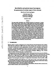
Escherichia coli is the most studied microorganism in the literature. Even so, its metabolic networks are not completely observable. For different experimental conditions, there are several infrequent or absent measures of intracellular metabolites. Thus, some studies have focused on the development of kinetic model for metabolic network for this microorganism (e.g., Chassagnole et al. [2]; di Maggio et al. [40]; Degenring [41]; Usuda et al. [42]). Particularly, E. coli K-12 W3110 to be wild type (wt) corresponds to standard strain that can be genetically manipulated allowing a large range of applications, such as: (i) pharmaceutical, recombinants proteins, vaccines, and serums, (ii) genetic medicine, (iii) environmental, biomarkers and pollution-fighting, and (v) energetic, biodiesel, oils, and others. E. coli is able to metabolize a large variety of components (e.g., carbohydrates, proteins, amino acids, lipids, and organics acids), produce catalase, and also utilize a variety of sources (e.g., glucose, ammonia, and nitrogen). Besides, E. coli grows in large concentrations allowing fermentative processes of high yield [43]. Regarding parameters identifiability in E. coli, di Maggio et al. [40] used global sensitivity analysis proposed by Sobol’ [44] to determine the most influential parameters on the dynamics of the central carbon metabolism of this bacterium, based on the model proposed by Chassagnole et al. [2]. di Maggio et al. [40] concluded that twelve kinetic parameters were the most influential for the model predictions. These parameters represent maximum reaction rates, inhibition, and half-saturation constants. Their identification and later estimation provide the starting points for the manipulation of certain enzyme properties [40]. Large scale metabolic network of the glycolysis, the pentose-phosphate-pathway, and the phosphotransferase system of E. coli K-12 W3110 (Figure 4) [40] consists of a complex mathematical structure with 18 dynamic mass balance equations, (5) to (22) presented below, 7 additional algebraic equations, (A.1) to (A.7), and 30 kinetic rate expressions, (A.8) to (A.37) [2]. Some enzyme kinetics modifications were introduced by di Maggio et al. [40] as the kinetic expression for the activity of phosphofructokinase was taken from Ricci [45] (see (A.12)) and the activity of glucose-6-phosphate dehydrogenase was modeled by the expression proposed by Ratushny et al. [46] (see (A.13)).
fructose-6-phosphate: f6p 𝑑𝐶f6p 𝑑𝑡
= 𝑟PGI − 𝑟PFK + 𝑟TKb + 𝑟TA − 2𝑟MurSynth − 𝜇𝐶f6p , (7)
fructose-1,6-biphosphate: fdp 𝑑𝐶fdp 𝑑𝑡
= 𝑟PKF − 𝑟ALDO − 𝜇𝐶fdp ,
(8)
glyceraldehyde-3-phosphate: gap 𝑑𝐶gap
= 𝑟ALDO + 𝑟TIS − 𝑟GAPDH + 𝑟TKa
𝑑𝑡
(9)
+ 𝑟TKb − 𝑟TA + 𝑟TrpSynth − 𝜇𝐶gap , dihydroxyacetonephosphate: dhap 𝑑𝐶dhap 𝑑𝑡
= 𝑟ALDO − 𝑟TIS − 𝑟G3PDH − 𝜇𝐶dhap ,
(10)
1,3-diphosphoglycerate: pgp 𝑑𝐶pgp
= 𝑟GAPDH − 𝑟PGK − 𝜇𝐶pgp ,
𝑑𝑡
(11)
3-phosphoglycerate: 3pg 𝑑𝐶3pg 𝑑𝑡
= 𝑟PGK − 𝑟PGGluMu − 𝑟SerSynth − 𝜇𝐶3pg ,
(12)
2-phosphoglycerate: 2pg 𝑑𝐶2pg
= 𝑟PGluMu − 𝑟ENO − 𝜇𝐶2pg ,
𝑑𝑡
(13)
phosphoenolpyruvate: pep 𝑑𝐶pep
= 𝑟ENO − 𝑟PK − 𝑟PTS − 𝑟PEPCxylase
𝑑𝑡
(14)
− 𝑟DAHPS − 𝑟Synth1 − 𝜇𝐶pep , pyruvate: pyr
Mass Balances to the Substrate (See (5)) and Intracellular Metabolites (See (6)–(22))
𝑑𝑡
glucose: glc extracellular 𝑑𝐶glc
𝑑𝑡
feed extracellular ) + 𝑓pulse − − 𝐶glc = 𝐷 (𝐶glc
𝑑𝐶pyr
= 𝑟PK + 𝑟PTS − 𝑟PDH − 𝑟Synth2
𝐶𝑥 𝑟PTS , 𝜌𝑥 (5)
6-phosphogluconate: 6pg 𝑑𝐶6pg 𝑑𝑡
glucose-6-phosfato: g6p 𝑑𝐶g6p 𝑑𝑡
(15)
+ 𝑟MetSynth + 𝑟TrpSynth − 𝜇𝐶pyr ,
= 𝑟PTS − 𝑟PGI − 𝑟G6PDH − 𝑟PGM − 𝜇𝐶g6p ,
= 𝑟G6PDH − 𝑟PGDH − 𝜇𝐶6pg ,
(16)
ribulose-5-phosphate: ribu5p (6)
𝑑𝐶ribu5p 𝑑𝑡
= 𝑟PGDH − 𝑟Ru5P − 𝑟R5PI − 𝜇𝐶ribu5p ,
(17)
BioMed Research International
9 Glucose
pep
PTS
pyr
g1p
PGM
g6p
G6PDH
6pg
PGDH
ribu5p
PGI
G1PAT
Polysaccharides th f6p rSyn synthesis ATP Mu PFK Mureine ADP synthesis fdp
xyl5p
dhap
PI rib5p
RPPK
Tka Tkb
Gap
sed7p
Nucleotides synthesis
TA
ALDO Glycerol G3PDH synthesis
R5
5P Ru
TIS
pep
GAPDH
Tryptophan synthesis
pgp ADP
SerSynth
3pg
DAHPS
Aromatic amino acids synthesis
PGK
ATP
f6p
e4p
Gap
Serine synthesis
PGIuMu 2pg ENO PEPCxylase pep oaa th1 Syn Mureine PK and chorismate synthesis pyr
ADP ATP Syn th
2
PDH
Amino acids synthesis
AcCoA
Figure 4: Escherichia coli central carbon metabolism [2].
xylulose-5-phosphate: xyl5p 𝑑𝐶xyl5p 𝑑𝑡
= 𝑟Ru5P − 𝑟TKa − 𝑟TKb − 𝜇𝐶xyl5p ,
erythrose-4-phosphate: e4p (18)
𝑑𝑡
= 𝑟TKa − 𝑟TA − 𝜇𝐶sed7p ,
(19)
ribose-5-phosphate: rib5p 𝑑𝐶rib5p 𝑑𝑡
= 𝑟R5PI − 𝑟TKa − 𝑟RPPK − 𝜇𝐶rib5p ,
𝑑𝑡
= 𝑟TA − 𝑟TKb − 𝑟DAHPS − 𝜇𝐶e4p ,
(21)
glucose-1-phosphate: g1p
sedoheptulose-7-phosphate: sed7p 𝑑𝐶sed7p
𝑑𝐶e4p
(20)
𝑑𝐶glp 𝑑𝑡
= 𝑟PGM − 𝑟GIPAT − 𝜇𝐶glp .
(22)
As usual, the values of initial estimates used here were found in the literature [40]. Experimental data employed in this work were obtained in Hoque et al. [43] throughout a time horizon of 300 seconds. Temporal profiles for glucose
10
BioMed Research International 25
Collinearity angle (∘ ) 0.5 175.3 176.5 179.5 176.5 179.3 2.5 0.0 179.3 2.5 177.4 2.4 1.6 177.5 2.3 1.5 0.7 175.2 177.6
20
Parameters par 𝐾PTS,1 − 𝐾PTS,3 max 𝐾ALDO,eq − 𝑟TIS 𝐾GAPDH,nad − 𝐾PGK,eq 𝐾GAPDH,eq − 𝐿 PK max 𝐾PK,amp − 𝑟PGM 𝐾GIPAT,glp − 𝐾GIPAT,atp max 𝐾PK,amp − 𝑟Ser,Synth 𝐾PK,fdp − 𝐾Synth1,pep 𝑛DAHPS,pep − 𝐾ALDO,fdp 𝐾GAPDH,eq − 𝐾G6PDH,tgn 𝐿 PK − 𝐾G6PDH,tgn 𝐾PGDH,atp − 𝐾G1PAT,g1p 𝐾PGDH,atp − 𝐾G1PAT,atp 𝐾PGDH,atp − 𝐾PGDH,nadp 𝐾TA,eq − 𝐾G1PAT,g1p 𝐾TA,eq − 𝐾G1PAT,atp 𝐾TA,eq − 𝐾PGDH,atp max − 𝐾G6PDH,dt 𝑟PTS max − 𝐾GAPDH,nad 𝑟PGDH
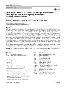
(glc), dihydroxyacetonephosphate (dhap), erythrose-4-phosphate (e4p), pyruvate (pyr), fructose-1,6-diphosphate (fdp), ribose-5-phosphate (rib5p), ribulose-5-phosphate (ribu5p), 2-phosphoglycerate (2pg), phosphoenolpyruvate (pep), glyceraldehyde-3-phosphate (gap), glucose-6-phosphate (g6p), fructose-6-phosphate (f6p), and 6-phosphogluconate (6pg) were used for parameters identifiability. As a previous analysis, the collinearity angle among sensitivity vectors for all parameters of the model were calculated, and the frequency of each angle interval is shown in Figure 5. The results indicate high frequency of parameters pars linearly independents (collinearity angles values approximately 90∘ ), in this way Table 1 presents few parameters pars with critical collinearity angles values that do not expect to be selected until a first successfully performed selection. Fifty eight parameters have been identified, together with five initial conditions of metabolites concentrations which were not known from experimental data (pgp = 1.215 × 10⁻⁵ , 3pg = 1.911, xyl5p = 1.564, sed7p = 4.085 × 10⁻² , and g1p = 6.500 × 10⁻² ). In metabolic networks, the initial conditions of intracellular metabolites are very important. It is not recommended to keep initial conditions of unknown metabolites at zero, because numerical problems in model integration can occur or predicted values can become unreliable. In such situations, the initial concentrations of unknown metabolites must be estimated together with the parameters. In order to obtain a first initial estimates of nonmeasured intracellular metabolites, the following procedures were employed in this paper: (i) initially, keep the initial concentrations of nonmeasured intracellular metabolites at zero and simulate the model until next integration point (first
Frequency (%)
Table 1: Parameters pars of the E. coli K-12 W3110 metabolic networks with critical collinearity angles values.
15
10
5
0
0
50
100 150 Collinearity angle (∘ )
200
Figure 5: Collinearity angles among sensitivity vectors 𝑏𝜃𝑖 and 𝑏𝜃𝑗 for all parameters of the E. coli K-12 W3110 metabolic networks.
numerical integration step must be small), and (ii) take the calculated values for the nonmeasured intracellular metabolites concentrations as initial conditions; the information obtained in (ii) is given as initial estimates of concentrations of nonmeasured intracellular metabolites in the identifiability procedure. Numerical results for the proposed procedure are presented in Figure 6 and Table 2, comparing the model simulation with initial parameters estimates from the literature [40] and reestimated parameters according to the intensive parameters evaluation. Figure 6 demonstrates the improvement of the model prediction by using the proposed procedure of parameters identifiability. Unfortunately, model limitations and few experimental data impose some insurmountable barriers to identifiability procedures. Thus, some metabolites did not change after applying the identifiability procedure. In this way, the 10 metabolites profiles that were significantly improved after the identifiability procedure are presented. Since the model fits reasonably the experimental data, it can be concluded that the parameters selection was performed with relatively good success. A special attention should be given to Figures 6(b), 6(d), and 6(f) for which the mathematical model behavior using initial estimates of parameters values is not able to follow the tendency of the experimental data. For these cases, the initial estimates of parameters values showed to be inadequate. Table 2 presents the estimated parameters together with the initial estimates and their normalized standard deviations, calculated as the ratio between the standard deviation of the parameter and its estimated value (𝜎𝜃 /𝜃). As important information of the identifiable parameters, the low normalized relative deviations obtained after the numerical procedure indicates a good quality of the estimated values. Analyzing the parameters estimated values, it is found that initial estimates of the parameters were significantly improved. It is important to emphasize that the estimates of the selected parameters can be significantly influenced by the initial estimates of the nonselected parameters. Thus,
BioMed Research International
11
Table 2: Identifiable parameters of the E. coli K-12 W3110 metabolic networks obtained using the numerical procedure for intensive parameters evaluation. Parameter 𝐾PTS1 max 𝑟PDH max 𝑟ALDO max 𝑟G6PDH 𝐾R,pep max 𝑟GAPDH 𝐾PEPCxylase,fdp 𝐾R5P,eq 𝑛PEPCxylase,fdp max 𝑟PK 𝑛PDH 𝐾PGI,f6p2 𝑘tgn 𝐾G3PDH,dhap max 𝑟TA 𝑘hdt 𝐾PGI,g6p 𝐾PGI,f6p 𝐾TKA,eq 𝐾PGLUMU,2pg 𝐾R5PI,eq max 𝑟TKA max 𝑟RU5PI max 𝑟R5PI max 𝑟PFK 𝐾PGI,g6p2 𝐿 PK 𝐾Synthesis1,pep 𝐾PEPCxylase,pep 𝑛DAHPS,e4p 𝑛DAHPS,pep 𝑒 𝐾T,pep 𝐾GAPDH,nadh 𝐾PGK,3pg 𝑛PK ℎhdt 𝐾TIS,gap ℎtgn 𝑛G1PAT,fdp 𝐸 𝐾TA,eq 𝐾PGLUMU,3pg 𝜃 𝐾T,adp 𝐾TIS,dhap max 𝑟PTS 𝐾PGLUMU,eq 𝑛PTS,g6p
Initial estimate 3082.300 4.010 30.423 12.873 750.000 500.000 0.700 1.400 4.000 0.567 1.000 0.200 1.000 1.000 8.461 0.100 0.400 0.266 0.120 0.369 4.000 7.372 5.182 3.733 1.967 0.200 1.000 1.000 4.070 2.600 2.200 0.999 0.750 1.090 0.473 4.000 4.000 0.300 2.000 2.000 0.990 1.050 0.200 1.000 1.300 2.800 82107.310 0.187 4.000
Estimated value 3683.300 0.529 1.593 8.476 0.541 0.381 0.469 0.647 8.795 0.140 7.237 1.271 4.152 19.076 4.051 0.099 0.060 1.956 × 10⁻⁴ 6.289 1.105 4.182 1.461 0.100 1.366 0.382 0.272 785.758 0.361 5.731 3.501 3.455 1.057 0.630 4.752 2.326 1.582 0.584 0.567 9.169 5.993 0.114 2.583 0.084 1.506 1.145 7.830 1.876 0.626 0.443
Normalized standard deviation 0.060 0.015 0.081 0.041 0.051 0.021 0.028 0.064 0.041 0.069 0.028 0.037 0.075 0.110 0.051 0.038 0.101 0.115 0.050 0.039 0.052 0.069 0.054 0.019 0.057 0.193 0.070 0.053 0.038 0.022 0.032 0.054 0.122 0.027 0.077 0.030 0.136 0.050 0.057 0.084 0.078 0.054 0.035 0.065 0.123 0.057 0.070 0.066 0.037
12
BioMed Research International Table 2: Continued.
Parameter 𝐾PTS,g6p 𝐾PKA,adp 𝐾PKA,adp 𝐾GAPDH,nad 𝐾ALDO,gap2 𝐾PK,atp 𝐾PGDH,6pg max 𝑟PGLUMU max 𝑟PGDH
Initial estimate 0.393 0.260 0.400 0.252 1.200 22.500 5.449 96.972 5.221
Estimated value 0.366 0.208 0.455 0.093 0.240 1.483 3.597 0.749 0.597
more adequate parameters values can be obtained when a large experimental dataset is available, allowing estimating all parameters of the mathematical model. Using the proposed numerical procedure, the objective function was also improved in two orders of magnitude relative to the initial estimates. The results are also dependent on the assumed behavior of experimental uncertainties. It is usual to assume the standard deviation of the dependent variable (𝜎𝑦𝑖 ) to be proportional to its value (𝑦𝑖 ) in the form 𝜎𝑦𝑖 = 𝑎 ⋅ 𝑦𝑖 + 𝑏,
(23)
where 𝑎 and 𝑏 are generally arbitrarily chosen. For example, for 𝑎 = 1 × 10⁻¹ and 𝑏 = 1 × 10⁻⁵ , the initial value of the objective function was 1.56 × 10⁴ and reduced to 3.06 × 10³ after reestimation. For 𝑎 = 1 × 10⁻² and 𝑏 = 1 × 10⁻⁶ , the initial value of the objective function was 3.89 × 10⁷ and reduced to 3.06 × 10⁵ after parameters reestimation. The set of selected parameters was not the same in both cases; nevertheless, the prediction was similar. The dependence of parameters estimation performance on the assumed experimental uncertainties is expected even for well posed problems. It is important information, but generally it is neglected and arbitrarily chosen due to the difficulties involved in characterizing the experimental errors. Even with so much uncertainties, associated to experimental data, modeling development and some unknown initial conditions, it has been shown that it is possible to fit and/or improve model predictions with parameters identifiability procedures. The model can now be used for predicting the experimental behavior of the system. Besides its uncertainties, it can help to give us an idea about what we should expect in experimental regions, delimiting experimental design for further investigations, among other purposes. Naturally, for more accurate results, some predictions should be confirmed by additional experiments in the experimental regions of greater interest. Comparing the performance of the proposed numerical procedure with similar procedure but stopping the selection when the last selected parameter was not successfully included, only 63 parameters have been selected, and the objective function was around 5 times greater compared with the results obtained with the algorithm presented in Figure 2. It emphasizes the necessity to investigate all parameters in
Normalized standard deviation 0.080 0.063 0.056 0.070 0.125 0.062 0.051 0.063 0.036
order to improve final results and not to stop the procedure when the first parameter have failed to be included. In the procedure proposed in previous work [18], subsets of parameters were included at once, and if the estimation of such subset was possible, this subset could not leave the set of selected parameters. Thus, if a set of parameters has been successfully estimated, the orthogonalization step (for discount parameters influence one each other) was not performed between such parameters. In the procedure presented in this work, one parameter is selected each time, and orthogonalization step between the selected parameters and yet unselected parameters is performed much more times than in previous work [18]. Although not assured by the model nonlinearities, one can expect that the present procedure should lead to better results, despite being more time consuming, since it performs a more thorough investigation regarding the parameters correlation. In fact, the objective function obtained in this work divided by the objective function of previous work [18] was 0.15, indicating a good improvement in prediction performance. It is important to emphasize that, for this application, the improvement in the prediction quality was observed with estimation of only half of the model parameters, being the numerical procedure performed using unknown values for some initial conditions of the dependent variables. Thus, in similar scenarios, a great merit of the parameters identifiability procedure is to select only the most influential parameters on the mathematical model that can be estimated with the available experimental data.
5. Conclusion In this work, a large scale ill-posed problem of parameters estimation in metabolic networks was investigated, where experimental data are scarce and concentrations of intracellular metabolites are not completely known. A proposed procedure of intensive parameters evaluation that presents simultaneous parameters selection and estimation was successfully applied to solve this problem. Compared in pairs, few parameters seem to be correlated, as revealed by collinearity angles. From the initial scenario, containing 131 parameters and 5 unknown initial conditions of intracellular metabolites concentrations, the procedure was able to identify 58 parameters, together with the 5 initial conditions
13
0.8
15
0.6
10 5 0
0.6 0.5 Ce4p (mM)
20
Cdhap (mM)
Cglc (mM)
BioMed Research International
0.4 0.2
0
100
200
0
300
0
100
6
1.5
4
1
0
300
0
100
200
0.5
0
300
(e)
2.5 C6pg (mM)
2 C2pg (mM)
1.5
0.5
1.5 1
0
300
200 Time (s)
300
2 1.5
0.5 200 Time (s)
100
(f)
2.5
100
0
Time (s)
1
300
1
3
0
200
1.5
2
0
100 (c)
0.5
2
200 Time (s)
0
Time (s)
Crib5p (mM)
2
Cpyr (mM)
Cfdp (mM)
8
100
0.1
300
(b)
(d)
Cribu5p (mM)
200 Time (s)
(a)
0
0.3 0.2
Time (s)
0
0.4
0
(g)
100
200 Time (s)
300
1
0
100
200
300
Time (s)
(h)
(i)
0.8
Cpep (mM)
0.6 0.4 0.2 0
0
100
200
300
Time (s) (j)
Figure 6: Experimental and predicted metabolites concentrations as function of the time: (I) experimental value, (--) predicted value using initial estimates, and (-e-) predicted value after parameter identifiability using model of E. coli K-12 W3110 metabolic networks.
14
BioMed Research International
Table 3: Kinetics parameters. Enzyme
Parameter
Description
Phosphotransferase system: PTS
𝐾PTS1 𝐾PTS2 𝐾PTS3 𝐾PTS,g6p 𝑛PTS,g6p max 𝑟PTS
M–M half-saturation constant (mM) Constant (mM) Constant Inhibition constant (mM) Constant Maximum reaction rate (mM s−1 )
Phosphoglucoisomerase: PGI
𝐾PGI,g6p 𝐾PGI,f6p 𝐾PGI,eq 𝐾PGI,g6p,6pg,inh 𝐾PGI,f6p,6pg,inh max 𝑟PGI
M–M half-saturation constant (mM) Inhibition constant (mM) Equilibrium constant Inhibition constant (mM) Inhibition constant (mM) Maximum reaction rate (mM s−1 )
Phosphofructokinase: PFK
𝐾PFK,f6p,s 𝐾PFK,atp,s 𝐾PFK,adp,a 𝐾PFK,adp,b 𝐾PFK,adp,c 𝐾PFK,amp,a 𝐾PFK,amp,b 𝐾PFK,pep 𝐿 PFK 𝑛PFK max 𝑟PFK
M–M half-saturation constant (mM) M–M half-saturation constant (mM) Activation constant (mM) Activation constant (mM) Activation constant (mM) Activation constant (mM) Activation constant (mM) Inhibition constant (mM) Allosteric constant Number of binding sites Maximum reaction rate (mM s−1 )
Aldolase: ALDO
𝐾ALDO,fdp 𝐾ALDO,dhap 𝐾ALDO,gap 𝐾ALDO,gap,inh 𝑉ALDO,blf 𝐾ALDO,eq max 𝑟ALDO
M–M half-saturation constant (mM) M–M half-saturation constant (mM) M–M half-saturation constant (mM) Inhibition constant (mM) Back-forward reaction rate relation Equilibrium constant (mM) Maximum reaction rate (mM s−1 )
Triosephosphate isomerase: TIS
𝐾TIS,dhap 𝐾TIS,gap 𝐾TIS,eq max 𝑟TIS
M–M half-saturation constant (mM) M–M half-saturation constant (mM) Equilibrium constant Maximum reaction rate (mM s−1 )
Glyceraldehyde-3-phosphate dehydrogenase: GAPDH
𝐾GAPDH,gap 𝐾GAPDH,pgp 𝐾GAPDH,nad 𝐾GAPDH,nadh 𝐾GAPDH,eq max 𝑟GAPDH
M–M half-saturation constant (mM) Inhibition constant (mM) M–M half-saturation constant (mM) Inhibition constant (mM) Equilibrium constant Maximum reaction rate (mM s−1 )
Phosphoglycerate kinase: PGK
𝐾PGK,pgp 𝐾PGK,3pg 𝐾PGK,adp 𝐾PGK,atp 𝐾PGK,eq max 𝑟PGK
M–M half-saturation constant (mM) Inhibition constant (mM) M–M half-saturation constant (mM) Inhibition constant (mM) Equilibrium constant Maximum reaction rate (mM s−1 )
BioMed Research International
15 Table 3: Continued.
Enzyme
Parameter
Description
Phosphoglycerate mutase: PGluMu
𝐾PGluMu,3pg 𝐾PGluMu,2pg 𝐾PGluMu,eq max 𝑟PGluMu
M–M half-saturation constant (mM) Inhibition constant (mM) Equilibrium constant Maximum reaction rate (mM s−1 )
Enolase: ENO
𝐾ENO,2pg 𝐾ENO,pep 𝐾ENO,eq max 𝑟ENO
M–M half-saturation constant (mM) Inhibition constant (mM) Equilibrium constant Maximum reaction rate (mM s−1 )
Pyruvate kinase: PK
𝐾PK,pep 𝐾PK,adp 𝐾PK,atp 𝐾PK,fdp 𝐾PK,amp 𝐿 PK 𝑛PK max 𝑟PK
M–M half-saturation constant (mM) M–M half-saturation constant (mM) Inhibition constant (mM) Activation constant (mM) Activation constant (mM) Allosteric constant Number of binding sites Maximum reaction rate (mM s−1 )
Pyruvate dehydrogenase: PDH
𝐾PDH,pyr 𝑛PDH max 𝑟PDH
M–M half-saturation constant (mM) Number of binding sites Maximum reaction rate (mM s−1 )
Phoenolpyruvate carboxylase: PEPCxylase
𝐾PEPCxylase,pep 𝐾PEPCxylase,fdp 𝑛PEPCxylase,fdp max 𝑟PEPCxylase
M–M half-saturation constant (Mm) Activation constant (mM) Number of binding sites Maximum reaction rate (mM s−1 )
Phosphoglucomutase: PGM
𝐾PGM,g6p 𝐾PGM,g1p 𝐾PGM,eq max 𝑟PGM
M–M half-saturation constant (mM) Inhibition constant (mM) Equilibrium constant Maximum reaction rate (mM s−1 )
Glucose-1-phosphate adenyltransferase: G1PAT
𝐾G1PAT,g1p 𝐾G1PAT,atp 𝐾G1PAT,fdp 𝑛G1PAT,fdp max 𝑟G1PAT
M–M half-saturation constant (mM) M–M half-saturation constant (mM) Activation constant (mM) Number of binding sites Maximum reaction rate (mM s−1 )
Ribose phosphate pyrophosphokinase: RPPK
𝐾RPPK,rib5p max 𝑟RPPK
M–M half-saturation constant (mM) Maximum reaction rate (mM s−1 )
Glycerol-3-phosphate dehydrogenase: G3PDH
𝐾G3PDH,dhap max 𝑟G3PDH
M–M half-saturation constant (mM) Maximum reaction rate (mM s−1 )
Serine synthesis: SerSynth
𝐾SerSynth,3pg max 𝑟SerSynth
M–M half-saturation constant (mM) Maximum reaction rate (mM s−1 )
DAHP synthase: DAHPS
𝐾DAHPS,e4p 𝐾DAHPS,pep 𝑛DAHPS,e4p 𝑛DAHPS,pep max 𝑟DAHPS
M–M half-saturation constant (mM) M–M half-saturation constant (mM) Number of binding sites Number of binding sites Maximum reaction rate (mM s−1 )
Glucose-6-phosphate dehydrogenase: G6PDH
𝐾G6PDH,g6p 𝐾G6PDH,nadp 𝐾G6PDH,nadph,nadph,inh 𝐾G6PDH,nadph,g6ph,inh max 𝑟G6PDH
M–M half-saturation constant (mM) M–M half-saturation constant (mM) Inhibition constant (mM) Inhibition constant (mM) Maximum reaction rate (mM s−1 )
16
BioMed Research International Table 3: Continued.
Enzyme
Parameter
Description
6-Phosphogluconate dehydrogenase: PGDH
𝐾PGDH,6pg 𝐾PGDH,nadp 𝐾PGDH,nadph,inh 𝐾PGDH,atp,inh max 𝑟PGDH
M–M half-saturation constant (mM) M–M half-saturation constant (mM) Inhibition constant (mM) Inhibition constant (mM) Maximum reaction rate (mM s−1 )
Ribulose phosphate epimerase: RU5P
𝐾RU5P,EQ max 𝑟RU5PI
Equilibrium constant (mM) Maximum reaction rate (mM s−1 )
Ribose phosphate isomerase: R5PI
𝐾R5PI,eq max 𝑟R5PI
Equilibrium constant (mM) Maximum reaction rate (mM s−1 )
Transketolase a: TKa
𝐾TKa,eq max 𝑟TKa
Equilibrium constant (mM) Maximum reaction rate (mM s−1 )
Transketolase b: TKb
𝐾TKb,eq max 𝑟TKb
Equilibrium constant (mM) Maximum reaction rate (mM s−1 )
Transaldolase: TA
𝐾TA,eq max 𝑟TA
Equilibrium constant (mM) Maximum reaction rate (mM s−1 )
Synthesis 1: Synth1
𝐾Synth1,pep max 𝑟Synth1
M–M half-saturation constant (mM) Maximum reaction rate (mM s−1 )
Synthesis 2: Synth2
𝐾Synth2,pyr max 𝑟Synth2
M–M half-saturation constant (mM) Maximum reaction rate (mM s−1 )
Mureine synthesis: MurSynth
max 𝑟MurSynth
Maximum reaction rate (mM s−1 )
Tryptophan synthesis: TrpSynth
max 𝑟TrpSynth
Maximum reaction rate (mM s−1 )
Methionine synthesis: MetSynth
max 𝑟MetSynth
Maximum reaction rate (mM s−1 )
of intracellular metabolites concentrations. The simultaneous reestimation step reduced the dependence on the initial parameters estimates, allowing a good fit of the model. The robustness of the applied procedure is certainly an appealing feature for metabolic networks problems.
diphosphopyridine nucleotide phosphate, reduced: nadph 𝐶nadph = 0.062 + 0.332 (2.718−0.46𝑡 ) × (0.0166𝑡1.58 + 0.000166𝑡4.73
Appendix
+ 1.16 × 10⁻¹⁰ 𝑡7.89 + 1.36 × 10⁻¹³ 𝑡11
Time Correlations for Cometabolites Concentrations [2]
+ 1.23 × 10⁻¹⁶ 𝑡14.2 ) , diphosphopyridine nucleotide, reduced: nadp
Adenosintriphosphate: atp 𝐶atp
𝑡 = 4.27 − 4.163 , 0.657 + 1.43𝑡 + 0.364𝑡2
(A.1)
𝐶nadp = 0.159 + 0.00554 + 0.182
adenosindiphosphate: adp 𝐶adp = 0.582 + 1.73 (2.731−0.15𝑡 ) (0.12𝑡 + 0.000214𝑡3 ) , (A.2) adenosin monophosphate: amp 𝐶amp = 0.123 + 7.25
𝑡 7.25 + 1.47𝑡 + 0.17𝑡2
𝑡 + 1.073 , 1.29 + 8.05𝑡
(A.4)
𝑡 2.8 + 0.271𝑡 + 0.01𝑡2
𝑡 , 4.81 + 0.526𝑡
(A.5)
diphosphopyridine nucleotide, reduced: nadh 𝐶nadh = 0.0934 + 0.0011 (2.371−0.123𝑡 ) (0.844𝑡 + 0.104𝑡3 ) , (A.6) diphosphopyridine nucleotide, oxized: nad 𝐶nad = 1.314 + 1.314 (2.73(−0.0435𝑡−0.342) )
(A.3) −
(𝑡 + 7.871) (2.73(−0.0218𝑡−0.171) ) 8.481 + 𝑡
(A.7) .
BioMed Research International
17
Kinetics Rates for Enzymes [2, 40]. Consider max extracelular 𝑟PTS = 𝑟PTS 𝐶glc
max (𝐶fdp − 𝑟ALDO = 𝑟ALDO
𝐶gap 𝐶dhap
𝐶pep
× ((𝐾PTS1 + 𝐾PTS2
𝐶pep
+
𝐶pyr
extracelular extracelular + 𝐾PTS,3 𝐶glc + 𝐶glc
𝐶pep 𝐶pyr
)
+
−1
𝑛
× (1 +
PTS,g6p 𝐶g6p
𝐾PTS,g6p
𝐾ALDO,eq 𝑉ALDO,blf 𝐶gap
𝑟PGI =
(𝐶g6p −
𝐾PGI,eq
× (𝐾PGI,g6p (1+
+
𝐾ALDO,gap,inh
) ,
)
𝐾TIS,eq
)
(A.11)
𝐶fdp 𝐶gap
−1
𝐶dhap 𝐶gap
× (𝐾TIS,dhap (1 +
𝐶f6p
+
𝐾ALDO,eq 𝑉ALDO,blf
max 𝑟TIS = 𝑟TIS (𝐶dhap −
)) ,
𝐾ALDO,eq 𝑉ALDO,blf
𝐾ALDO,dhap 𝐶gap
(A.8) max 𝑟PGI
𝐾ALDO,gap 𝐶dhap
× (𝐾ALDO,fdp + 𝐶fdp +
𝐶pyr
)
𝐾ALDO,eq
(A.12)
−1
𝐶gap
) + 𝐶dhap ) ,
𝐾TIS,gap
𝑟GAPDH 𝐶f6p
𝐾PGI,f6p (1+ (𝐶6pg /𝐾PGI,f6p,6pginh ))
𝐶pgp 𝐶nadh
max = 𝑟GAPDH (𝐶gap 𝐶nad −
𝐾GAPDH,eq
−1
𝐶6𝑝𝑔
× ((𝐾GAPDH,gap (1 +
) + 𝐶g6p ) ,
𝐾PGI,g6p,6pginh
(A.9) 𝑟PFK
)
𝐶pgp 𝐾GAPDH,pgp
) + 𝐶gap )
(A.13)
𝐶nadh ) 𝐾GAPDH,nadh
× (𝐾GAPDH,nad (1 + −1
+ 𝐶nad )) ,
[ 𝑛PFK −1 𝑒𝐶 𝐶adp 𝑛PFK 𝑒𝐶 max [ [ f6p (1 + f6p ) = 𝑟PFK (1 + ) [𝐾 𝐾Rf6p 𝐾Radp [ Rf6p [ + 𝐿0 [
× 𝜃𝑐𝑒
(1+ (𝐶pep /𝐾Tpep )) (1+ (𝐶adp /𝐾Tadp )) (1+ (𝐶pep /𝐾Rpep )) (1+ (𝐶adp /𝐾Radp )) 𝐶f6p 𝐾Rf6p
(1 + 𝑐𝑒
𝑛PFK −1
𝐶f6p 𝐾Rf6p
)
𝑛PFK
]
𝑒𝐶f6p 𝐾Rf6p
+ 𝐿0 [
𝑛PFK
)
(1 +
𝐶adp 𝐾Radp
] ] ] ] ]
max (𝐶3pg − 𝑟PGluMu = 𝑟PGluMu
× (1 + 𝑐𝑒
𝐾Rf6p
𝐶pep /𝐾Tpep
)
𝐶atp 𝐾PGK,atp
) + 𝐶adp )
𝐶3pg 𝐾PGK,3pg
𝐶2pg 𝐾PGluMu,eq
𝑛PFK
)
× (𝐾PGluMu,3pg (1 +
(1 + (𝐶pep /𝐾Rpep )) (1 + (𝐶adp /𝐾Radp )) 𝐶f6p
× ((𝐾PGK,adp (1 +
)
−1
) + 𝐶pgp )) , (A.14)
(1 + (𝐶pep /𝐾Tpep )) (1 + (𝐶adp /𝐾Tadp ))
𝐾PGK,eq
× (𝐾PGK,pgp (1 +
] × ( (1 +
𝐶atp 𝐶3pg
max 𝑟PGK = 𝑟PGK (𝐶adp 𝐶pgp −
)
𝐶2pg 𝐾PGluMu,2pg
−1
) + 𝐶3pg ) , (A.15)
𝑛PFK
]
max (𝐶2pg − 𝑟ENO = 𝑟ENO
𝐶pep 𝐾ENO,eq
−1
) ,
× (𝐾ENO,2pg (1 + (A.10)
)
𝐶pep 𝐾ENO,pep
−1
) + 𝐶2pg ) , (A.16)
18
BioMed Research International 𝑟PK
𝑟PGDH
max = 𝑟PK 𝐶pep 𝐶adp (
max = 𝑟PGDH 𝐶6pg 𝐶nadp
(𝑛PK −1)
𝐶pep 𝐾PK,pep
+ 1)
× ((𝐶6pg + 𝐾PGDH,6pg )
× (𝐾PK,pep
× (𝐶nadp + 𝐾PGDH,nadp
× (𝐿 PK (1 +
𝐶atp 𝐾PK,atp
×(
+(
× (1 +
𝐶fdp
𝐶amp
+
𝐾PK,fdp
𝐾PK,amp
× (1 +
𝑛PK
−1
+ 1) )
𝐶pep
+ 1)
𝐾PK,pep
𝐶nadph
𝐾PGDH,atp,inh
max 𝑟RU5P = 𝑟RU5P (𝐶ribu5p −
× (𝐶adp + 𝐾PK,adp ) ) ,
max (𝐶rib5p 𝐶xyl5p − 𝑟TKa = 𝑟TKa
(A.17) max 𝑛PDH 𝑟PDH 𝐶pyr
𝑟PDH =
𝐾PDH,pyr +
𝑛PDH 𝐶pyr
,
max (𝐶xyl5p 𝐶e4p − 𝑟TKb = 𝑟TKb
(A.18)
max 𝑟TA = 𝑟TA (𝐶gap 𝐶sed7p −
𝑟G6PDH max = 𝑟GPDH 𝐶g6p
−1
𝐶atp
)
−1
)
𝐾PGDH,nadph,inh
max 𝑟R5PI = 𝑟R5PI (𝐶ribu5p −
𝑛PK
(A.20)
))) ,
𝐶rib5p 𝐾R5PI,eq
𝐶xyl5p 𝐾RU5P,eq
),
),
𝐶sed7p 𝐶gap 𝐾TKa,eq 𝐶f6p 𝐶gap
𝐾TA,eq
(A.22)
(A.23)
),
(A.24)
),
(A.25)
𝐾TKb,eq 𝐶e4p 𝐶f6p
),
(A.21)
𝑟PEPCxylase
× ((𝐾G6PDH,g6p (1 +
× (1 +
× ((
ℎtg 𝐶nadp 𝑘tgn ℎ ) ℎtg 𝑘tgtg + 𝐶nadp
𝐶nadph 𝐾G6PDH,nadphinh
𝐾G6PDH,nadp
× ((1 + (
)
ℎ
𝐾PEPCxylase,pep + 𝐶pep
)
𝐾G6PDH,nadh
𝑟SerSynth =
ℎ
)
𝑟RPPK = ℎnadph
)
𝐾G6PDH,nadphinh2 𝐶nadh
ℎ
dt dt 1+𝑘dtn (𝐶nadh /(𝑘dtdt +𝐶nadh ))
𝐾G6PDH,nadp
ℎnadh
)
𝑟G3PDH =
) −1
𝐾Synth1,pep + 𝐶pep
𝑟Synth2 =
ℎ
ℎ
max 𝑟Synth1 𝐶pep
𝑟Synth1 =
dt dt 1+𝑘dtn (𝐶nadh /(𝑘dtdt +𝐶nadh ))
𝐶nadp
𝑛PEPCxylase,fdp
)
,
(A.26)
𝐾G6PDH,nadhinh
𝐶nadph
× (1 + (
+ 𝐶g6p )
𝐶nadh
ℎ
𝐶nadp
+(
+
=
max 𝑟PEPCxylase 𝐶pep (1 + (𝐶fdp /𝐾PEPCxylase,fdp )
−1
)) )) , (A.19)
max 𝑟Synth2 𝐶pyr
𝐾Synth2,pyr + 𝐶pyr
,
(A.27)
,
(A.28)
max 𝑟SerSynth 𝐶3pg
𝐾SerSynth,3pg + 𝐶3pg max 𝐶rib5p 𝑟RPPK
𝐾RPPK,rib5p + 𝐶rib5p
,
,
max 𝐶dhap 𝑟G3PDH
𝐾G3PDH,dhap + 𝐶dhap
(A.29)
(A.30) ,
(A.31)
𝑟DAHPS 𝑛
=
𝑛
DAHPS,e4p DAHPS,pep max 𝐶e4p 𝐶pep 𝑟DAHPS
𝑛DAHPS,e4p 𝑛DAHPS,pep , (𝐾DAHPS,e4p + 𝐶e4p ) (𝐾DAHPS,pep + 𝐶pep ) (A.32)
BioMed Research International
𝑟PGM =
19
max 𝑟PGM (𝐶g6p − (𝐶g1p /𝐾PGM,eq ))
𝐾PGM,g6p (1 + (𝐶g1p /𝐾PGM,g1p )) + 𝐶g6p
,
(A.33)
𝑛G1PAT,fdp
𝑟G1PAT =
max 𝑟G1PAT 𝐶g1p 𝐶atp (1 + (𝐶fdp /𝐾G1PAT,fdp )
(𝐾G1PAT,g1p + 𝐶g1p ) (𝐾G1PAT,atp + 𝐶atp )
)
,
(A.34) 𝑟MurSynth =
max 𝑟MurSynth ,
max 𝑟TrpSynth = 𝑟TrpSynth ,
(A.36)
max 𝑟MetSynth = 𝑟MetSynth ,
(A.37)
Kinetics Parameters. See Table 3.
Nomenclature 𝜇: Specific growth rate or intracellular dilution rate 𝐷: Dilution rate. Metabolite Glc: g6p: f6p: Fdp: Gap: Dhap: Pgp: 3pg: 2pg: Pep: pyr: 6pg: ribu5p: xyl5p: sed7p: xyl5p: sed7p: rib5p: e4p: Glp:
Glucose Glucose-6-phosphate Fructose-6-phosphate Fructose-1,6-biphosphate Glyceraldehyde-3-phosphate Dihydroxyacetonephosphate 1,3-Diphosphoglycerate 3-Phosphoglicerate 2-Phosphoglicerate Phosphoenolpyruvate Pyruvate 6-Phosphogluconate Ribulose-5-phosphate Xylulose-5-phosphate Sedoheptulose-7-phosphate Xylulose-5-phosphate Sedoheptulose-7-phosphate Ribose-5-phosphate Erythrose-4-phosphate Glucose-1-phosphate.
Cometabolite Atp: Adp: Nad: Nadh: Nadp:
(A.35)
Adenosintriphosphate Adenosindiphosphate Diphosphopyridindinucleotide, oxized Diphosphopyridindinucleotide, reduced Diphosphopyridindinucleotide-phosphate, oxized Nadph: Diphosphopyridindinucleotide-phosphate, reduced Amp: Adenosinmonophosphate.
Enzyme ALDO: DAHPS: ENO: G1PAT: G3PDH: G6PDH: GAPDH: MetSynth: MurSynth: PDH: PEPCxylase: PFK: PGDH: PGI: PGK: PGM: PGluMu: PK: PTS: R5PI: RPPK: RU5P: SerSynth: Synth1: Synth2: TA: TIS: TKa: TKb: TrpSynth:
Aldolase DAHPS synthase Enolase Glucose-1-phosphate adenyltransferase Glycerol-3-phosphate dehydrogenase Glucose-6-phosphate dehydrogenase Glyceraldehyde 3-phosphate dehydrogenase Methionine synthesis Mureine synthesis Pyruvate dehydrogenase PEP carboxylase Phosphofructokinase 6-Phosphogluconate dehydrogenase Phosphoglucoisomerase Phosphoglycerate kinase Phosphoglucomutase Phosphoglycerate mutase Pyruvate kinase Phosphotransferase system Ribose phosphate isomerase Ribose phosphate pyrophosphokinase Ribulose phosphate epimerase Serine synthesis Synthesis 1 Synthesis 2 Transaldolase Triosephosphate isomerase Transketolase a Transketolase b Tryptophan synthesis.
Conflict of Interests The authors declare that there is no conflict of interests regarding the publication of this paper.
Acknowledgment The authors thank CNPq (Conselho Nacional de Desenvolvimento Cient´ıfico e Tecnol´ogico), CAPES (Coordenac¸a˜o de Aperfeic¸oamento de Pessoal de N´ıvel Superior), CONICET (National Research Council), and ANPCYT (Agencia Nacional de Promoci´on Cient´ıfica y Tecnol´ogica) for providing scholarships and for supporting this work.
References [1] R. Steuer and B. H. Junker, “Computational models of metabolism: stability and regulation in metabolic networks,” in Advances in Chemical Physics, S. A. Rice, Ed., pp. 6970–6992, John Wiley & Sons, New York, NY, USA, 2008. [2] C. Chassagnole, N. Noisommit-Rizzi, J. W. Schmid, K. Mauch, and M. Reuss, “Dynamic modeling of the central carbon metabolism of Escherichia coli,” Biotechnology and Bioengineering, vol. 79, no. 1, pp. 53–73, 2002.
20 [3] B. Ø. Palsson, Systems Biology—Properties of Reconstructed Networks, Cambridge University Press, New York, NY, USA, 2006. [4] R. S. Costa, D. Machado, I. Rocha, and E. C. Ferreira, “Critical perspective on the consequences of the limited availability of kinetic data in metabolic dynamic modelling,” IET Systems Biology, vol. 5, no. 3, pp. 157–163, 2011. [5] A. Buchholz, J. Hurlebaus, C. Wandrey, and R. Takors, “Metabolomics: quantification of intracellular metabolite dynamics,” Biomolecular Engineering, vol. 19, no. 1, pp. 5–15, 2002. [6] U. Schaefer, W. Boos, R. Takors, and D. Weuster-Botz, “Automated sampling device for monitoring intracellular metabolite dynamics,” Analytical Biochemistry, vol. 270, no. 1, pp. 88–96, 1999. [7] C. Kravaris, J. Hahn, and Y. Chu, “Advances and selected recent developments in state and parameter estimation,” Computers and Chemical Engineering, vol. 51, pp. 111–123, 2013. [8] D. E. Thompson, K. B. McAuley, and P. J. McLellan, “Parameter estimation in a simplified MWD model for HDPE produced by a ziegler-natta catalyst,” Macromolecular Reaction Engineering, vol. 3, no. 4, pp. 160–177, 2009. [9] F. P. Davidescu and S. B. Jørgensen, “Structural parameter identifiability analysis for dynamic reaction networks,” Chemical Engineering Science, vol. 63, no. 19, pp. 4754–4762, 2008. [10] R. T. Roper, M. P. Saccomani, and P. Vicini, “Cellular signaling identifiability analysis: a case study,” Journal of Theoretical Biology, vol. 264, no. 2, pp. 528–537, 2010. [11] I. E. Nikerel, W. A. van Winden, P. J. T. Verheijen, and J. J. Heijnen, “Model reduction and a priori kinetic parameter identifiability analysis using metabolome time series for metabolic reaction networks with linlog kinetics,” Metabolic Engineering, vol. 11, no. 1, pp. 20–30, 2009. [12] S. Srinath and R. Gunawan, “Parameter identifiability of powerlaw biochemical system models,” Journal of Biotechnology, vol. 149, no. 3, pp. 132–140, 2010. [13] H. Yue, M. Brown, J. Knowles, H. Wang, D. S. Broomhead, and D. B. Kell, “Insights into the behaviour of systems biology models from dynamic sensitivity and identifiability analysis: a case study of an NF-𝜅B signalling pathway,” Molecular BioSystems, vol. 2, no. 12, pp. 640–649, 2006. [14] A. R. Secchi, N. S. M. Cardozo, E. Almeida Neto, and T. F. Finkler, “An algorithm for automatic selection and estimation of model parameters,” in Proceedings of International Symposium on Advanced Control of Chemical Processes (ADCHEM ’06), pp. 789–794, Gramado, Brazil, 2006. [15] S. Wu, T. J. Harris, and K. B. McAuley, “The use of simplified or misspecified models: linear case,” Canadian Journal of Chemical Engineering, vol. 85, no. 4, pp. 386–398, 2007. [16] S. Wu, K. A. P. McLean, T. J. Harris, and K. B. McAuley, “Selection of optimal parameter set using estimability analysis and MSE-based model-selection criterion,” International Journal of Advanced Mechatronic Systems, vol. 3, no. 3, pp. 188–197, 2011. [17] K. A. P. McLean, S. Wu, and K. B. McAuley, “Mean-squarederror methods for selecting optimal parameter subsets for estimation,” Industrial and Engineering Chemistry Research, vol. 51, no. 17, pp. 6105–6115, 2012. [18] K. P. F. Alberton, A. L. Alberton, J. A. Di Maggio, M. S. D´ıaz, and A. R. Secchi, “Accelerating the parameters identifiability procedure: set by set selection,” Computers and Chemical Engineering, vol. 55, pp. 181–197, 2013.
BioMed Research International [19] S. R. Weijers and P. A. Vanrolleghem, “A procedure for selecting best identifiable parameters in calibrating activated sludge model no 1 to full-scale plant data,” Water Science and Technology, vol. 36, no. 5, pp. 69–79, 1997. [20] C. A. Sandink, K. B. McAuley, and P. J. McLellan, “Selection of parameters for updating in on-line models,” Industrial and Engineering Chemistry Research, vol. 40, no. 18, pp. 3936–3950, 2001. [21] R. J. Li, M. A. Henson, and M. J. Kurtz, “Selection of model parameters for off-line parameter estimation,” IEEE Transactions on Control Systems Technology, vol. 12, no. 3, pp. 402–412, 2004. [22] B. F. Lund and B. A. Foss, “Parameter ranking by orthogonalization: applied to nonlinear mechanistic models,” Automatica, vol. 44, no. 1, pp. 278–281, 2008. [23] Y. Chu and J. Hahn, “Parameter set selection for estimation of nonlinear dynamic systems,” AIChE Journal, vol. 53, no. 11, pp. 2858–2870, 2007. [24] R. Brun, P. Reichert, and H. R. K¨unsch, “Practical identifiability analysis of large environmental simulation models,” Water Resources Research, vol. 37, no. 4, pp. 1015–1030, 2001. [25] K. Z. Yao, B. M. Shaw, B. Kou, K. B. McAuley, and D. W. Bacon, “Modeling ethylene/butene copolymerization with multi-site catalysts: parameter estimability and experimental design,” Polymer Reaction Engineering, vol. 11, no. 3, pp. 563–588, 2003. [26] C. Sun and J. Hahn, “Parameter reduction for stable dynamical systems based on Hankel singular values and sensitivity analysis,” Chemical Engineering Science, vol. 61, no. 16, pp. 5393–5403, 2006. [27] Y. Chu, Z. Huang, and J. Hahn, “Global sensitivity analysis procedure accounting for effect of available experimental data,” Industrial and Engineering Chemistry Research, vol. 50, no. 3, pp. 1294–1304, 2011. [28] Y. Bard, Nonlinear Parameter Estimation, Academic Press, New York, NY, USA, 1974. [29] A. L. Alberton, M. Schwaab, M. W. N. Lob˜ao, and J. C. Pinto, “Experimental design for the joint model discrimination and precise parameter estimation through information measures,” Chemical Engineering Science, vol. 66, no. 9, pp. 1940–1952, 2011. [30] L. R. Petzold, “A description of DASSL: a differential/algebraic systems solve,” in Scientific Computing, R. S. Stepleman et al., Ed., pp. 65–68, North Holland Publishing, Amsterdam, The Netherlands, 1989. [31] M. Schwaab, A. L. Alberton, and J. C. Pinto, “ESTIMA&PLANEJA: Pacote computacional para estimac¸a˜o de parˆametros de planejamento de experimentos,” Internal Technical Report, Universidade Federal do Rio de Janeiro, Rio de Janeiro, Brazil, 2010. [32] J. Kennedy and R. Eberhart, “Particle swarm optimization,” in Proceedings of the IEEE International Conference on Neural Networks, vol. 4, pp. 1942–1948, Perth, Wash, USA, NovemberDecember 1995. [33] D. E. Goldberg, Genetic Algorithms in Search, Optimization and Machine Learning, Addison Wesley Longman, Boston, Mass, USA, 1989. [34] W. B. Copeland, B. A. Bartley, D. Chandran et al., “Computational tools for metabolic engineering,” Metabolic Engineering, vol. 14, no. 3, pp. 270–280, 2012. [35] W. Wiechert and A. A. Graaf, “Bidirectional reaction steps in metabolic networks: I. modeling and simulation of carbon isotope labeling experiments,” Biotechnology and Bioengineering, vol. 55, pp. 101–117, 1997.
BioMed Research International [36] Z. P. Gerdtzen, P. Daoutidis, and W.-S. Hu, “Non-linear reduction for kinetic models of metabolic reaction networks,” Metabolic Engineering, vol. 6, no. 2, pp. 140–154, 2004. [37] W. Wiechert, C. Siefke, A. A. de Graaf, and A. Marx, “Bidirectional reaction steps in metabolic networks: II. Flux estimation and statistical analysis,” Biotechnology and Bioengineering, vol. 55, pp. 118–135, 1997. [38] M. M¨ollney, W. Wiechert, D. Kownatzki, and A. A. Graaf, “Bidirectional reaction steps in metabolic networks: IV. Optimal design of isotopomer labeling experiments,” Biotechnology and Bioengineering, vol. 66, no. 2, pp. 86–103, 1999. [39] K. N¨oh and W. Wiechert, “Experimental design principles for isotopically instationary 13C labeling experiments,” Biotechnology and Bioengineering, vol. 94, no. 2, pp. 234–251, 2006. [40] J. di Maggio, J. C. Diaz Ricci, and M. S. Diaz, “Global sensitivity analysis in dynamic metabolic networks,” Computers and Chemical Engineering, vol. 34, no. 5, pp. 770–781, 2010. [41] D. Degenring, Erstellung und validierung mechanistischer modelle f¨ur den mikrobiellen stoffwechsel zur auswertung von substrat-puls-experimenten [M.S. thesis], University of Rostock, Rostock, Germany, 2004. [42] Y. Usuda, Y. Nishio, S. Iwatani et al., “Dynamic modeling of Escherichia coli metabolic and regulatory systems for aminoacid production,” Journal of Biotechnology, vol. 147, no. 1, pp. 17– 30, 2010. [43] M. A. Hoque, H. Ushiyama, M. Tomita, and K. Shimizu, “Dynamic responses of the intracellular metabolite concentrations of the wild type and pykA mutant Escherichia coli against pulse addition of glucose or NH3 under those limiting continuous cultures,” Biochemical Engineering Journal, vol. 26, no. 1, pp. 38–49, 2005. [44] I. M. Sobol’, “Global sensitivity indices for nonlinear mathematical models and their Monte Carlo estimates,” Mathematics and Computers in Simulation, vol. 55, no. 1–3, pp. 271–280, 2001. [45] J. C. D. Ricci, “Influence of phosphoenolpyruvate on the dynamic behavior of phosphofructokinase of Escherichia coli,” Journal of Theoretical Biology, vol. 178, no. 2, pp. 145–150, 1996. [46] A. Ratushny, O. Smirnova, Y. Usuda, and K. Matsui, “Regulation of the pentose phosphate pathway in Escherichia coli: gene network reconstruction and mathematical modeling of metabolic reactions,” in Proceedings of the International Conference on Bioinformatics of Genome Regulation and Structure (BGRS ’06), pp. 40–44, Novosibirsk, Russia, 2006.
21