Simultaneous estimation of the parameters of the Hurst ... - ITIA

Simultaneous estimation of the parameters of the Hurst-Kolmogorov stochastic process Hristos Tyralis and Demetris Koutsoyiannis Department of Water Resources, Faculty of Civil Engineering, National Technical University, Athens Heroon Polytechneiou 5, GR-157 80 Zographou, Greece ([email protected])

Abstract Various methods for estimating the self-similarity parameter (Hurst parameter, H) of a Hurst-Kolmogorov stochastic process (HKp) from a time series are available. Most of them rely on some asymptotic properties of processes with Hurst-Kolmogorov behaviour and only estimate the self-similarity parameter. Here we show that the estimation of the Hurst parameter affects the estimation of the standard deviation, a fact that was not given appropriate attention in the literature. We propose the Least Squares based on Variance estimator, and we investigate numerically its performance, which we compare to the Least Squares based on Standard Deviation estimator, as well as the maximum likelihood estimator after appropriate streamlining of the latter. These three estimators rely on the structure of the HKp and estimate simultaneously its Hurst parameter and standard deviation. In addition, we test the performance of the three methods for a range of sample sizes and H values, through a simulation study and we compare it with other estimators of the literature. Key words Hurst phenomenon; Hurst-Kolmogorov behaviour; long term persistence; hydrological statistics; hydrological estimation; Hurst parameter estimators.

INTRODUCTION Hurst (1951) discovered a behaviour of hydrological and other geophysical time series, which has become known with several names such as Hurst phenomenon, long-term persistence and long-range dependence, and has subsequently received extensive attention in the literature.

2 Earlier, Kolmogorov (1940), when studying turbulence, had proposed a mathematical model to describe this behaviour, which was further developed by Mandelbrot and van Ness (1968) and has been known as simple scaling stochastic model or fractional Gaussian noise (see Beran 1994; Embrechts and Maejima 2002; Palma 2007; Doukhan et al. 2003; Robinson 2003; and the references therein). Here the behaviour is referred to as the Hurst-Kolmogorov (HK) behaviour or HK (stochastic) dynamics and the stochastic model as the HK process (HKp). A lot of studies on this kind of behaviour regarding actual data have been accomplished. To mention two of the most recent, Buette et al. (2006) studied the Irish daily wind speeds, using ARFIMA and GARMA models, whereas Zhang et al. (2009) studied the scaling properties of the hydrological series in the Yellow River basin. Of critical importance in analyzing hydrological and geophysical time series is the estimation of the strength of the HK behaviour. The parameter H, known as the Hurst or self-similarity parameter of the HKp arises naturally from the study of self-similar processes and expresses the strength of the HK behaviour. A number of estimators of H have been proposed. These are usually validated by an appeal to some aspect of self-similarity, or by an asymptotic analysis of the distributional properties of the estimator as the length of the time series converges to infinity. Rea et al. (2009) present an extensive literature review dealing with the properties of these estimators. They also examine the properties of twelve estimators, i.e. the nine more classical estimators (aggregated variance, differencing the variance, absolute values of the aggregated series, Higuchi’s method, residuals of regression, R/S method, periodogram method, modified periodogram method, Whittle estimator) discussed in Taqqu et al. (1995) plus the wavelet, GPH and Haslett-Raftery estimator. Weron (2002) discusses the properties of residuals of regression, R/S method and periodogram method. Grau-Carles (2005) also analyzes the behaviour of the residuals of regression, the R/S method and the GPH.

3 Besides new estimators are proposed, for example Guerrero and Smith (2005) presented a maximum likelihood based estimator, while Coeurjolly (2008) presented estimators based on convex combinations of sample quantiles of discrete variations of a sample path over a discrete grid of the interval [0, 1]. Some authors propose improvements of existing estimators. For example, Mielniczuk and Wojdyllo (2007) improve the R/S method. Other authors like Esposti et al. (2008) propose methodologies which use more than one methods simultaneously to estimate the H parameter. Because the finite sample properties of these estimators can be quite different from their asymptotic properties, some authors have undertaken empirical comparisons of estimators of H. The nine classical estimators were discussed in some detail by Taqqu et al. (1995) who carried out an empirical study of these estimators for a single series length of 10 000 data points, 5 values of H, and 50 replications. All twelve above estimators were discussed in more detail by Rea et al. (2009) who carried out an empirical study of these estimators for series lengths between 100 and 10 000 data points in steps of 100, H values between 0.55 and 0.90 in steps of 0.05 and 1000 replications. Rea et al. (2009) also presented an extensive literature review about the same kind of empirical studies. These studies did not include two methods. The maximum likelihood (ML) method discussed by McLeod and Hippel (1978) and McLeod et al. (2007), probably due to computational problems (Beran 1994, p. 109), and the method by Koutsoyiannis (2003), hereinafter referred to as the LSSD (Least Squares based on Standard Deviation) method, which was also articulated recently by Ehsanzadeh and Adamowski (2010). The ML method estimates the Hurst parameter based on the whole structure of the process, i.e. its joint distribution function. The LSSD method relies on the self-similarity property of the process. One common characteristic of the ML and LSSD methods is that they estimate simultaneously the Hurst parameter H and the standard deviation σ of the process. This is of

4 great importance, because both parameters are essential for the construction of the model and, as we will show below (see also Koutsoyiannis 2003) their estimators generally are not independent to each other. In addition, the classical statistical estimator of σ encompasses strong bias if applied to a series with HK behaviour (Koutsoyiannis 2003; Koutsoyiannis and Montanari 2007). It is thus striking that some of the existing methods do not remedy or even pose this problem at all, and estimate H independently of σ and vice versa, e.g. assuming that σ can be estimated using its classical statistical estimator, which does not depend on H. The focus of this paper is the simultaneous estimation of the parameters H and σ of the HKp. We use the ML and LSSD methods that have the capacity of simultaneous estimation, after appropriate streamlining of the former in a more practical form, and we propose a third method which is an improvement of the LSSD method (referred to as LSV method —Least Squares based on Variance) retaining the simultaneous parameter estimation attitude. We apply the three methods to evaluate their performance in a Monte Carlo simulation framework and we compare the results with those of the estimators presented in Taqqu et al. (1995) with the exception of the Whittle estimator, which we replaced by the local Whittle estimator presented in Robinson (1995).

METHODS Definition of HKp Let Xi denote a stochastic process with i = 1, 2, … denoting discrete time. We assume that there is a record of n observations which we write as a vector xn = (x1 … xn)T (where the superscript T is used to denote the transpose of a vector or matrix). We recall from statistical theory that each observation xi represents a realization of a random variable Xi, so that xn is a realization of a vector of identically distributed random variables Xn = (X1 … Xn)T (notice the upper- and lower-case symbols used for random variables and values thereof, respectively,

5 and the arrangement of the sample members and observations from the latest to the earliest). It is assumed that the process is stationary, a property that does not hinder to exhibit multiple scale variability. Further, let its mean be denoted as µ := E[Xi], its autocovariance γj := Cov[Xi, Xi + j], its autocorrelation ρj := Corr[Xi, Xi + j] = γj / γ0 (j = 0, ±1, ±2, …), and its standard deviation σ := γ0. Let k be a positive integer that represents a timescale larger than 1, the original time scale of the process Xi. The mean aggregated stochastic process on that timescale is denoted as ik

(k)

X i := (1/k)

∑

Xl l = (i – 1) k + 1

The notation implies that a superscript (1) could be omitted, i.e. X

(1)

(1) i

≡ Xi. The statistical

(k)

characteristics of X i for any timescale k can be derived from those of Xi. For example, the mean is (k)

E[X i ] = µ

(2)

whilst the variance and autocovariance (or autocorrelation) depend on the specific structure of γj (or ρj). Now we consider the following equation that defines the HKp: H

(k) (X i

d  k  (X(l) − µ), 0 < H < 1, − µ) =  l j  

(3)

d stands for equality in (finite dimensional joint) distribution and H is the where the symbol = Hurst parameter. We assume that equation (3) holds for any integer i and j (that is, the process is stationary) and any timescales k and l (≥ 1) and that Xi is Gaussian. We also define the aggregated stochastic process for every time scale:

(k)

Z i :=

ik

(k)

∑ Xl = k X i l = (i – 1) k + 1

(4)

6 For this process the following relationships hold: (k)

(k)

(k) 1/2

(k)

E[Z i ] = k µ, γ 0 = Var[Z i ] = k2·H γ0, σ(k) = (γ 0 ) (k)

(5)

(k)

The autocorrelation function of either of X i and Z i , for any aggregated timescale k, is independent of k, and given by (k)

ρ j = ρj = |j + 1|2H / 2 + |j − 1|2H / 2 − |j|2H

(6)

Maximum likelihood estimator In this section the method of maximum likelihood is employed for the estimation of the parameters of HKp, namely H, σ, µ. For a given record of n observations xn = (x1 … xn)T the likelihood of θ := (µ, σ, H) takes the general form (McLeod and Hippel 1978): 1 p(θ|xn) = (2π)n/2 [det(σ2 R)]−1/2 exp[−1/(2σ2) (xn − µ e)T R−1 (xn − µ e)]

(7)

where e = (1 1 … 1)T is a column vector with n elements, R is the autocorrelation matrix, i.e., a n x n matrix with elements rij = ρ|i − j|, and det( ) denotes the determinant of a matrix. ^ ), as shown in Appendix A, consists of Then a maximum likelihood estimator θ^ = (µ^, σ^, H the following relationships: T ^ −1 ^µ = x n R e, ^σ = ^ −1 e eT R

^ −1 (x − µ^ e) (xn − µ^ e)T R n n

(8)

^ can be obtained from the maximization of the single-variable function g (H) defined as: and H 1 T

T

n x n R−1 e T −1 x n R−1 e 1 g1(H) := − 2 ln[(xn − eT R−1 e e) R (xn − eT R−1 e e)] − 2 ln[det(R)]

(9)

LSSD method This method was proposed by Koutsoyiannis (2003). In his paper after a systematic Monte

7 ~ Carlo study he found an estimator S of σ, approximately unbiased for known H and for normal distribution of Xi, where

~ S :=

n – 1/2 S= n − n2H − 1

n − 1/2 (n − 1) (n − n2H − 1)

1 S2 := n − 1

n

(n)

∑ (Xi − X 1 )2

n

(n)

∑ (Xi − X 1 )2

(10)

i=1

(11)

i=1

(n)

and X 1 from equation (1) equals the sample mean. This algorithm is based on classical sample estimates s(k) of standard deviations σ(k) for timescales k ranging from 1 to a maximum value k΄ = [n/10]. This maximum value was chosen so that s(k) can be estimated from at least 10 data values. ~ Combining (5) and (10), assuming E[S] = σ and using the self-similarity property of the process one obtains E[S(k)] ≈ ck(H) kH σ with

ck(H) :=

n/k − (n/k)2H − 1 n/k − 1/2

(12)

Then the algorithm minimizes a fitting error e2(σ, H): k' [lnσ + H · lnk + lnc (H) – lns(k)]2 [lnE[S(k)] − lns(k)]2 Hq+1 Hq+1 k e (σ, H) := ∑ + = + (13) kp q+1 k∑ kp q+1 k=1 =1 2

k'

where a weight equal to 1/kp is assigned to the partial error of each scale k. For p = 0 the weights are equal whereas for p = 1, 2, …, decreasing weights are assigned to increasing scales; this is reasonable because at larger scales the sample size is smaller and thus the uncertainty larger. Using Monte Carlo experiments it was found that, although differences in estimates caused by different values of p in the range 0 to 2 are not so important, p = 2 results in slightly more efficient estimates (i.e., with smaller variation) and thus is preferable. A

8 penalty factor Hq+1/(q+1) has been included in e2 in (13) for a high q, say 50. The effect of this ^ = 1 and forces H ^ to slightly smaller values when it is factor is that it excludes the value H close to 1. As a consequence this factor helps get rid of an infinite σ^ also forcing to smaller ^ close to 1 (see Appendix B). values for H An analytical procedure to locate the minimum is not possible. Therefore, minimization of e2(σ, H) is done numerically and several numerical procedures can be devised for this purpose. A detailed iterative procedure is given in Koutsoyiannis (2003). LSV method ~ In the previous method an approximately unbiased estimator S of σ was found after a systematic Monte Carlo simulation. However, if σ2 is used instead of σ, we have the advantage that there exists a theoretically consistent expression, which determines E[S2] as a function of σ and H. This is the basis to form a modified version of the LSSD method, the LSV method. From the general relationship (Beran 1994, p. 9) δn(ρ) 2 E[S2] = (1− n – 1) σ , where δn(ρ) := (1/n)

n−1

∑ ρ(i, j) = 2 ∑ (1 − i≠j

k=1

k n) ρ(k)

(14)

we easily obtain that for an HKp: n − n2H−1 2 E[S ] = n − 1 σ 2

(15)

Due to the self-similarity property of the process the following relationship holds: E[S2(k)] = where

(n/k) − (n/k)2H−1 (k) (n/k) − (n/k)2H−1 2H 2 γ0 = k σ = ck(H) k2H σ2 (n/k) − 1 (n/k) − 1

(16)

9 ck(H) :=

n/k (k) (n) (n/k) − (n/k)2H−1 1 and S2(k) = (Z i − k X 1 )2. ∑ (n/k) − 1 n/k − 1 i = 1

(17)

Thus, the following error function should be minimized in order to obtain an estimation of H and σ:

e2(σ, H) :=

k' [c (H) k2H σ2 − s2(k)]2 [E[S2(k)] − s2(k)]2 k = , k΄ = [n/10] p ∑ ∑ k kp k=1 k=1 k'

(18)

Taking partial derivatives, i.e., ∂e2(σ, H) = 2 [σ2 α11(H) − α12(H)] ∂σ2

(19)

where: k' c (H) k2H s2(k) c2k(H) k4H k , α p 12(H) := ∑ k kp k=1 k=1 k'

α11(H) :=

∑

(20)

and equating to zero we obtain an estimate of σ: σ^ =

^ )/α (H ^) α12(H 11

(21)

An estimate of H can be obtained by minimizing the single-variable function: 2 s4(k) α12 (H) g2(H) := ∑ kp − α (H) , 0 < Η < 1 11 k=1 k'

(22)

^ = We prove in Appendix B that e2(σ, H) attains its minimum for H ≤ 1. However, when H 1, then from equations (21) and (31) we obtain that σ^ = ∞. Accordingly, to avoid such behaviour (values of σ^ tending to infinity), a penalty factor Hq+1/(q+1) for a high q is added again, as in method LSSD, to the error function. So the function to be minimized becomes:

10 e2(σ, H) :=

[ck(H) k2H σ2 − s2(k)]2 Hq+1 + ∑ kp q+1 k=1 k'

(23)

An estimate of H can be obtained by the minimization of the single-variable function: 2 s4(k) α12 (H) Hq+1 g2(H) := ∑ p − + ,0 1 and σ2 > 0 (It’s easy to prove that an estimated σ^ > 0 always). Now for 2

any H1 ∈ (0, 1) we can always find a σ1 > 0, such that ck(H1) k2H1 σ1 − s2(k) < 0 for every k. For 2

2

these values of H1 and σ1: | ck(H1) k2·H1 σ1 − s2(k) | < | ck(H2) k2·H2 σ2 − s2(k) | for every k. This

17 proves that e2(σ1, H1) < e2(σ2, H2). Thus, e2(σ, H) attains its minimum for H ≤ 1.

APPENDIX C: Calculation of Fisher Information Matrix’s elements We can easily calculate the I12(θ), I13(θ) and I23(θ) elements of the Fisher Information Matrix (Robert 2007, p. 129): T −1 ∂ln[p(θ|xn)] 1 T −1 = − 2 (e R e µ − x n R e) ∂µ σ

(32)

∂ln[p(θ|xn)] n 1 = − σ + σ3 (xn − µ e)T R−1 (xn − µ e) ∂σ

(33)

T −1 ∂2ln[p(θ|xn)] 2 T −1 = 3 (e R e µ − x n R e) ∂µ ∂σ σ

(34)

T ∂2ln[p(θ|xn)] 1 ∂R −1 ∂R −1 = 2 (µ eT R−1 R e − xn R−1 R e) ∂µ ∂H σ ∂H ∂H

(35)

∂2ln[p(θ|xn)] 1 T −1 ∂R −1 = − 3 (xn − µ e) R ∂σ ∂H σ ∂H R (xn − µ e)

(36)

The expectations of the above expressions are easily calculated and give the corresponding elements of the Fisher Information Matrix I(θ). Acknowledgements: The authors wish to thank two anonymous reviewers for their constructive comments.

REFERENCES Beran J (1994) Statistics for Long-Memory Processes, Volume 61 of Monographs on Statistics and Applied Probability. Chapman and Hall, New York Bouette JC, Chassagneux JF, Sibai D, Terron R, Charpentier R (2006) Wind in Ireland: long memory or seasonal effect. Stoch Environ Res Risk Assess 20(3):141-151 Coeurjolly JF (2008) Hurst exponent estimation of locally self-similar Gaussian processes

18 using sample quantiles. Ann Statist 36(3):1404-1434 Cox DR, Reid N (1987) Parameter Orthogonality and Approximate Conditional Inference. Journal of the Royal Statistical Society, Series B. (Methological) 49(1):1-39 Doukhan P, Oppenheim G, Taqqu M (2003) Theory and Applications of Long-Range Dependence. Birkhauser Ehsanzadeh E, Adamowski K (2010) Trends in timing of low stream flows in Canada: impact of autocorrelation and long-term persistence. Hydrol Process 24:970–980 Embrechts P, Maejima M (2002) Self similar Processes. Princeton University Press Esposti F, Ferrario M, Signorini MG (2008) A blind method for the estimation of the Hurst exponent in time series: Theory and application. Chaos 18(3). doi:10.1063/1.2976187 Grau-Carles P (2005) Tests of Long Memory: A Bootstrap Approach. Stoch Environ Res Risk Assess 25(1-2):103-113 Guerrero A, Smith L (2005) A maximum likelihood estimator for long-range persistence. Physica A 355(2-4):619-632 Hurst HE (1951) Long term storage capacities of reservoirs. Trans ASCE 116:776-808 Kolmogorov AE (1940) Wienersche Spiralen und einige andere interessante Kurven in Hilbertschen Raum. Dokl Akad Nauk URSS 26:115–118 Koutsoyiannis D (2003a) Climate change, the Hurst phenomenon, and hydrological statistics. Hydrol Sci J 48(1):3-24 Koutsoyiannis D (2003b) Internal report: http://www.itia.ntua.gr/getfile/537/2/2003HSJHurstSuppl.pdf Koutsoyiannis D, Montanari A (2007) Statistical analysis of hydroclimatic time series: Uncertainty

and

insights.

10.1029/2006WR005592

Water

Resour

Res

43(5).

W05429,

doi:

19 Mandelbrot BB, JW van Ness (1968) Fractional Brownian motion, fractional noises and applications. SIAM Rev 10:422–437 McLeod AI, Hippel K (1978) Preservation of the Rescaled Adjusted Range 1. A Reassesment of the Hurst Phenomenon. Water Resour Res 14(3):491-508 McLeod AI, Yu H, Krougly Z (2007) Algorithms for linear time series analysis: With R package. Journal of Statistical Software 23(5):1-26 Mielniczuk J, Wojdyllo P (2007) Estimation of Hurst exponent revisited. Computational Statistics & Data Analysis 51(9):4510-4525 Musicus B (1988) Levinson and Fast Cholesky Algorithms for Toeplitz and Almost Toeplitz Matrices. Research Laboratory of Electronics Massachusetts Institute of Technology. RLE Technical Report No. 538 Palma W (2007) Long-Memory Time Series Theory and Methods. Wiley-Interscience. Rea W, Oxley L, Reale M, Brown J (2009) Estimators for long range dependence: an empirical study. Electronic Journal of Statistics. arXiv:0901.0762v1 Robert C (2007) The Bayesian Choice: From Decision-Theoretic Foundations to Computational Implementation. Springer ,New York Robinson PM (1995) Gaussian semiparametric estimation of time series with long-range dependence. Ann Statist 23:1630-1661 Robinson PM (2003) Time Series with Long Memory. Oxford University Press Taqqu M, Teverovsky V, Willinger W (1995) Estimators for long-range dependence: an empirical study. Fractals 3(4):785-798 Weron R (2002) Estimating long-range dependence: finite sample properties and confidence intervals. Physica A: Statistical Mechanics and its Applications 312(1,2):285-299

20 Zhang Q, Xu CY, Yang T (2009) Scaling properties of the runoff variations in the arid and semi-arid regions of China: a case study of the Yellow River basin. Stoch Environ Res Risk Assess 23(8):1103-1111

21 0.2 0.6 0.4

0

0.2 ∆σ

∆H

0.1

-0.1 Median -0.2

0 -0.2

75% CI

-0.4

95% CI -0.3

-0.6

0.2 0

2000

4000

6000

8000

0

0.4

0

0.2 ∆σ

∆H

0.1

-0.1

2000

0.6

Series Length

.

4000

6000

8000

Series Length

0 -0.2

-0.2

-0.4

-0.3

-0.6

0.2 0

2000

4000

6000

8000

0

2000

0.6

Series Length 0.1

4000

6000

8000

Series Length

0.4 0.2 ∆σ

∆H

0 -0.1

0 -0.2

-0.2 -0.4 -0.3

-0.6 0

2000

4000

6000

Series Length

8000

0

2000

4000

6000

8000

Series Length

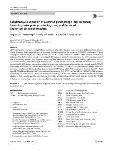
Fig. 1 Monte Carlo confidence intervals for the H and σ estimates with true H = 0.60, H = ^ − H, ∆σ = ^σ − σ, for the ML 0.90 and H = 0.95 (upper to lower panels), where ∆H = H estimator.

22 0.2 0.6 0.4

0

0.2 ∆σ

∆H

0.1

-0.1 Median -0.2

0 -0.2

75% CI

-0.4

95% CI -0.3

-0.6

0.2 0

2000

4000

6000

8000

0

0.4

0

0.2 ∆σ

∆H

0.1

-0.1

2000

0.6

Series Length

.

4000

6000

8000

Series Length

0 -0.2

-0.2

-0.4

-0.3

-0.6

0.2 0

2000

4000

6000

8000

0

2000

0.6

Series Length 0.1

4000

6000

8000

Series Length

0.4 0.2 ∆σ

∆H

0 -0.1

0 -0.2

-0.2

-0.4

-0.3

-0.6 0

2000

4000

6000

Series Length

8000

0

2000

4000

6000

8000

Series Length

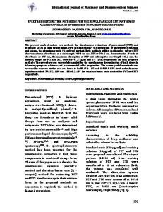
Fig. 2 Monte Carlo confidence intervals for the H and σ estimates with true H = 0.60, H = ^ − H, ∆σ = ^σ − σ, for the LSSD 0.90 and H = 0.95 (upper to lower panels), where ∆H = H estimator.

23 0.2 0.6 0.4

0

0.2 ∆σ

∆H

0.1

-0.1 Median -0.2

0 -0.2

75% CI

-0.4

95% CI -0.3

-0.6

0.2 0

2000

4000

6000

8000

0

0.4

0

0.2 ∆σ

∆H

0.1

-0.1

2000

0.6

Series Length

.

4000

6000

8000

Series Length

0 -0.2

-0.2

-0.4

-0.3

-0.6

0.2 0

2000

4000

6000

8000

0

2000

0.6

Series Length 0.1

4000

6000

8000

Series Length

0.4 0.2 ∆σ

∆H

0 -0.1

0 -0.2

-0.2

-0.4

-0.3

-0.6 0

2000

4000

6000

Series Length

8000

0

2000

4000

6000

8000

Series Length

Fig. 3 Monte Carlo confidence intervals for the H and σ estimates with true H = 0.60, H = ^ − H, ∆σ = ^σ − σ, for the LSV 0.90 and H = 0.95 (upper to lower panels), where ∆H = H estimator.

24 0.35

0.12 LSV

0.28

LSSD

0.09

RMSE

RMSE

ML

0.06

0.03

0.21 0.14 0.07 0

0 0.12 0

2000

4000

6000

8000

0.35

0

2000

Series Length

6000

8000

0.28 RMSE

0.09 RMSE

4000

Series Length

0.06

0.21 0.14

0.03 0.07 0 0.12 0

2000

4000

6000

0 0.35 0

8000

Series Length

4000

6000

8000

Series Length 0.28 RMSE

0.09 RMSE

2000

0.06

0.21 0.14

0.03 0.07 0

0 0

2000

4000

6000

Series Length

8000

0

2000

4000

6000

8000

Series Length

Fig. 4 Root mean square error (RMSE) (left of the estimated H and right of the estimated σ) as a function of series length for all three estimators, with H = 0.60, H = 0.90 and H = 0.95 (upper to lower panels) and σ = 1.

25 0.35 0.12

0.28 RMSE

RMSE

0.09 0.06 0.03

0 0.5

0.6

0.7

0.8

0.9

1

0.5

True H

0.6

0.7

0.8

0.9

1

0.9

1

0.9

1

True H

0.35

0.12

0.28 RMSE

0.09 RMSE

0.14 0.07

0

0.06 0.03

0.21 0.14 0.07 0

0 0.6 length:64 length:128 length:256 length:512 length:1024 length:2048 length:4096 length:8192

0.12 0.09

0.7

0.8

0.9

0.5

1

True H

0.6

0.7

0.8

True H

0.35 0.28 RMSE

0.5

RMSE

0.21

0.06 0.03

0.21 0.14 0.07

0

0 0.5

0.6

0.7

0.8

True H

0.9

1

0.5

0.6

0.7

0.8

Truel H

Fig. 5 Root mean square error (RMSE) of H (left) and σ (right) as a function of true H for all lengths. Upper to lower panels correspond to ML, LSSD and LSV methods.

26 1.2 series length:64

1

series length:128

0.8

series length:1024

Estimated mean,µ

0.6

series length:8192

0.4 0.2 0 -0.2 -0.4 -0.6 -0.8 -1 0.4

0.5

0.6

0.7 0.8 Estimated Hurst Parameter,H

0.9

1

Fig. 6 Estimated Hurst parameter H versus estimated mean µ from the ML method from 200 ensembles of synthetic time series with various lengths for true H = 0.8.

27 1.5 1.4

series length:64

Estimated standard deviation,s

series length:128 1.3 1.2

series length:1024 series length:8192

1.1 1 0.9 0.8 0.7 0.6 1.5 0.4

0.5

0.6

0.7 0.8 Estimated Hurst Parameter,H

0.9

1

0.5

0.6

0.7 0.8 Estimated Hurst Parameter,H

0.9

1

Estimated standard deviation,s

1.4 1.3 1.2 1.1 1 0.9 0.8 0.7 0.6 0.4

Fig. 7 Estimated Hurst parameter H versus estimated standard deviation σ from the ML method from 200 ensembles of synthetic time series with various lengths. The upper diagram corresponds to true H = 0.8 and the lower diagram coresponds to true H = 0.6.

28 0.05

0.08 0.07

0

0.06

-0.05

τH

∆H

0.05 0.04 0.03 -0.1

0.02

H=0.7 H=0.8

0.01

H=0.9 H=0.95

-0.15

0 15

25

35

45

55

65

75

85

95 105

15

25

35

45

55

q

65

75

85

95 105

65

75

85

95 105

q 0.3

0

-0.1 τσ

∆σ

0.24 0.18 0.12 -0.2 0.06 -0.3

0 15

25

35

45

55

65

75

85

95 105

15

25

35

q

45

55 q

Fig. 8 Mean of the estimated ∆H and ∆σ (left) and their corresponding standard deviations ^ − H, ∆σ from 200 ensembles of synthetic time series 128 long (right) versus q, where ∆H = H = ^σ − σ, τH and τσ are standard deviations and p = 6 for the LSV estimator. Definition of symbols used: 200

τH :=

(1/(200-1))

∑ (∆Hk)2, τσ :=

k=1

200

(1/(200-1))

∑ (∆σ)2

k=1

29 0.03

0.12

0

0.1 0.08 τH

∆H

-0.03

0.06

-0.06 0.04

H=0.7

-0.09

H=0.8

0.02

H=0.9 H=0.95

-0.12

0 2

3

4

5

6

7

8

9

10

11

2

p

0.32

3

4

5

6

7

8

9

10

11

7

8

9

10

11

p

0.35

0.24 0.28

0.16

0.21

0

τσ

∆σ

0.08

0.14

-0.08 -0.16

0.07

-0.24 -0.32

0 2

3

4

5

6

7

8

9

10

11

p

2

3

4

5

6 p

Fig. 9 Mean of the estimated ∆H and ∆σ (left) and their corresponding standard deviations ^ − H, ∆σ from 200 ensembles of synthetic time series 128 long (right) versus p, where ∆H = H = ^σ − σ, τH and τσ are standard deviations and q = 50 for the LSV estimator. (See definition of symbols used in caption of Fig. 8).

30 0.03 0

0.025

τH

∆H

0.02 -0.01

-0.02

0.015 0.01

H=0.7

0.005

H=0.8 H=0.9

-0.03 1

10

100

0

1000

1

10

m

0.01

100

1000

100

1000

m

0.12

0 -0.01 τσ

∆σ

0.08 -0.02

0.04

-0.03 -0.04 1

10

100

1000

m

0 1

10 m

Fig. 10 Mean of the estimated ∆H and ∆σ (left) and their corresponding standard deviations ^ − H, from 200 ensembles of synthetic time series 1024 long (right) versus m, where ∆H = H ∆σ = σ^ − σ, τH and τσ are standard deviations, p = 6 and q = 50 for the LSV estimator. (See definition of symbols used in caption of Fig. 8).

31 Table 1 Estimation results for H using 200 independent realizations 8,192 long where τ is the standard deviation of the sample containing the estimated H’s. H’s were estimated using the Matlab central file exchange functions package “Hurst parameter estimate” written by Chu Chen

(http://www.mathworks.com/matlabcentral/fileexchange/19148-hurst-parameter-

estimate), except the local Whittle estimates, where the local Whittle estimator written by Shimotsu was used (http://qed.econ.queensu.ca/faculty/shimotsu/) Estimation method Variance

DiffVar

Absolute

Higuchi

Var. of Residuals

R/S

Periodogram

Modified Periodogram

Local Whittle

^ H τ RMSE ^ H τ RMSE ^ H τ RMSE ^ H τ RMSE ^ H τ RMSE ^ H τ RMSE ^ H τ RMSE ^ H τ RMSE ^ H τ RMSE

0.6 0.595 0.027 0.027 0.567 0.073 0.080 0.594 0.028 0.029 0.599 0.028 0.028 0.600 0.024 0.024 0.619 0.031 0.036 0.604 0.024 0.024 0.565 0.037 0.051 0.601 0.023 0.023

True H 0.7 0.8 0.687 0.775 0.027 0.026 0.030 0.036 0.667 0.771 0.068 0.067 0.076 0.073 0.686 0.775 0.027 0.028 0.031 0.038 0.696 0.798 0.029 0.040 0.029 0.040 0.702 0.801 0.028 0.030 0.028 0.030 0.706 0.784 0.032 0.031 0.033 0.035 0.708 0.809 0.023 0.025 0.024 0.026 0.661 0.752 0.038 0.037 0.054 0.060 0.700 0.804 0.023 0.022 0.023 0.023

0.9 0.850 0.027 0.057 0.864 0.061 0.070 0.849 0.029 0.059 0.888 0.044 0.046 0.896 0.027 0.027 0.854 0.032 0.055 0.912 0.024 0.027 0.847 0.034 0.063 0.902 0.021 0.021

Note: Variance: a method based on aggregated variance; DiffVar: a method based on differencing the variance; Absolute: a method based on absolute values of the aggregated series; Higuchi: a method based on finding the fractal dimension; Var. of Residuals: a method based on residuals of regression, also known as Detrended Fluctuation Analysis (DFA); R/S: the original method by Hurst, based on the rescaled range statistic; Periodogram: a method based

32 on the periodogram of the time series; Modified Periodogram: similar as the Periodogram method but with frequency axis divided into logarithmically equally spaced boxes and averaging the periodogram values inside the box (see details in Taqqu et al. 1995); Local Whittle: a semiparametric version of the Whittle estimator (see details in Robinson 1995).

Table 2 Estimation results for H using 200 independent realizations 8,192 long where τ is the standard deviation of the sample containing the estimated H’s. Estimation method Maximum Likelihood

Least Squares Standard Deviation

Least Squares Variation

^ H τ RMSE ^ H τ RMSE ^ H τ RMSE

0.6 0.599 0.008 0.008 0.599 0.011 0.011 0.599 0.009 0.009

Nominal H 0.7 0.8 0.700 0.799 0.007 0.008 0.007 0.008 0.699 0.799 0.011 0.015 0.012 0.015 0.700 0.800 0.008 0.011 0.008 0.011

0.9 0.899 0.007 0.007 0.892 0.015 0.017 0.895 0.014 0.015