Proceedings of the 2004 IEEE Conference on Cybernetics and Intelligent Systems Singapore, 1-3 December, 2004
SINGLE EXPONENTIAL SMOOTHING METHOD AND NEURAL NETWORK IN ONE METHOD FOR TIME SERIES PREDICTION Dimce Risteski Computer Science Department Faculty of Electrical Engineering Skopje, Macedonia
[email protected]
Andrea Kulakov Computer Sciencc Department Faculty of Electrical Engincering Skopje, Macedonia
[email protected]
Ahtruct- the purpose of this paper is to present a new method that combines statistical techniques and neural networks in one method for the better time series prediction. In this paper- we presented single exponential smoothing method (statistical technique) merged with feed forward back propagation neurat network in one method named as Smart Single Exponential Smoothing Method (SSESM). The basic idea of the new method is to learn from the mistakes. More specifically, our neural network learns from the mistakes made by the statistical techniques. The mistakes are made by the smoothing parameter, which is constant. In our method, the smoothing parameter is a variable. It is changed according to the prediction of the neural network. Experimental results show that the prediction with a variable smoothing parameter is better than with a constant smoothing parameter.
I. INTRODUCTION To stay competitive, companies must plan there activitics into the future. This planning is vital for the succcss on the market. Companies collects information about there activities as saics, expenses, profit and many other aspects of there operations. In the human nature is to usc past to predict the future. To do successful planning companies must predict the future. Time series data is an ordered sequence of values of a variable at equally spaced time intervals. The time serics prediction goal is to observe or model the existing data series to enable future unknown data values to bc forccastcd accurately. Examples of data series include financial data series (stocks, indices, rates, etc.), physically observed data series (sunspots, weather, etc.), and mathematical data series (Fibonacci sequence, integrals of differential equations, etc.). The phrase “time series” generically refers to any data series, whether or not the data are dependent on a certain time increment. To do time series prediction we can use many deferent forecasting techniques, which are based OR histaricaI time series data and the trends the data reveal. In modern research, different methods taken from a variety of fields are employed for this task [I].
Neural Networks (NN) has been widely used as time series forecasters: most often these are feed-forward networks [Z]. Typical examples of use of neural networks in financial
0-780386434/04/$20.00 0 2004 IEEE
Danco Davcev Computer Science Department Faculty of Electrical Engincering Skopjc, Macedonja
[email protected]
forecasting are explained in many papers, for instance in stock forecasting [7], bankmptcy prediction for credit risk [5] and some guidelines for financial forecasting [6]. Proposals for better time series forccasting with NN, are given in many research papers published on various international journals and conferences [3, 4, 1 I]. Reference [I31 gives guidelines and limitations in time series forecasting with fced-fonvard neural nehvorks. The conclusion from that paper is that fcedforward neural network are cxtremcly scnsitivc to architecture and parameter choicc. The f i b r e of neural networks timc series forecasting seems to be in more complex network types that mcrge other technologics with neural network. The example of that kind of time series prcdiction is given in [4] where the authors usc smoothing unit based on the wavelet multiresolution analysis to reduce the influence of noise in time series prediction with neural network . They merge two different technologies to make a better time series prediction. The other techniques that are used for the timc series prediction are statistical methods or techniques [ I 11. The most common used method for forecast involving time series are exponential smoothing [9]. Exponential smoothing is a statistical family of methods or techniques. The basic method of this family i s a Single Exponential Smoothing Method (SESM). Single exponential smoothing method is very popular statistical method for the prediction o f time-series. The basic idea of our method named as Smart Single ExponentiaI Smoothing Method (SSESM) was to learn from the error that the SESM produces and io prcdict that error. The error is made by smoothing parameter. If we choose the right smoothing parameter than we can make a better prediction. SESM uses smoothing parameter with a constant value. In our method the better prediction is provided by using the neural network which learns when to increase or decrease the smoothing parameter from the train data. The smoothing parameter i s changed according to the prediction of the neural network. The comparison of predictions of our method and SESM shows that our method makes better predictions. In the second section of this paper we present in more details the single exponential smoothing method, while the feed-foiward neuraI networks with back propagation training is described in section 3. In section 4 we present our method, while in section 5 the evaluation results are given. The last section concludes the paper.
74 1
To make meaningful forccasts, the neural network has to be trained on an appropriate data series. Examplcs in the form of pairs are extracted from the data series, where input and output are vectors equal in size to the numbcr of network inputs and outputs, respectively. Then, for every example, back propagation training consists of three steps:
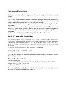
11. SINGEL EXPONENTIALSMOOTHING METHOD Exponential Smoothing is a very popular statistical family of techniques and scheme to produce a smoothed time series. This family of statistical tcchniques is the most common techniques for forecasts involving time series. Exponential smoothing assigns exponcntially decreasing weights as the observation get oldcr. in other words, recent observations havc relatively higher weights in forecasting than the older observations. In exponential smoothing there is one or more smoothing parameters to bc determined (or estimatcd) and these choices determine the wcights assigned to the observations .The single cxponential smoothing method is an exponential smoothing method with one smoothing parameter. The general formula for the calculations of the prediction of single exponential smoothing method is
Present an example’s input vector to the network inputs and run the nchvork: compute activation functions sequentially forward from the fust hidden layer to the output layer (Fig.1 from layer A to layer C). Compute the difference between the desired output for that example, output, and the actual network output (output of unit(s) in the output layer). Propagate the error sequentially backward from the output layer to the first hidden layer (Fig.] from layer C to layer A).
For every connection, change the weight modifying that connection in proportion to the error. where @O presents starting point value that usually is average of the data over some period, @I presents forecast for time period (L =l,2, ...), KO prescnts previous timc period‘s data value, Ki presents data value for time pcriod (I =1,2, ...),while a presents smoothing parameter which is a constant between 0 and I .
When these three steps have bccn performcd for evcry example from thc data serics, one epoch has occurred. Training usually lasts thousands of epochs; possibly until a prcdeterminqd maximum number of epochs (epochs limit) are reached or the network output error (error limit) falls below an acceptable threshold. Training can be time-consuming, depending on the network size, numbcr of examples, epochs limit, and error limit.
Equation ( I ) is a basic equation of exponential smoothing. One drawback of thc method is that we havc to use a great dcal of our data to calculate a starting point value (Qo) for the method. This value is usually the mean or average of the data over some period. A smoothing parameter denoted by a must be chosen to jump-start the forecast calculations. In the process of forecasting smoothing parameter is a constant. The smoothing parameter must be between 0 and 1 , The smaller parameter, the higher weight will be given to (initially) starting average (Qo). 111.
Over fitting is another major concept in the design of a NN. Ncural network that produces high forecasting error on unforeseen inputs, but low error on training inputs, is said to have over fitting the train data. When there is no enough data available to train the NN and the structure of NN is too complex, the NN tcnds to memorize the data rather than to generalize from it. Keeping the N N small is one way to avoid over fitting. In order to train NN better, all the data available should be used. To test the NN model, we partition the data into three parts. The first two parts are used to train (and validate) the NN while the third part of data is used to test the model. The NN is trained (with back propagation) directly on the training set, its generalization ability is monitored on the validation set, and its ability to forecast is measured on the test set. The general partition rule for training, validation and testing set is 70%, 20% and 10% respectively.
FEED-FORWARD BACKPROPAGATION NEURAL
NETWORK Nawrk
LayerA
To control over fitting, the following procedure to train the network we used: After every n epoch, we sum the total squared error for all examples from the training set. Also, sum the total squared error for all examples from the validation set.
Figure I . Feed-Forward Neural Network
Fig. 1 depicts an example feed-forward neural network. A neural network (”) can have any number of layers, units per layer, network inputs, and network outputs. This network has four units in the first layer (layer A) and three units in the second layer (layer E), which are called hidden layers. This network has one unit in the thud layer (layer C), which is called the output layer. Finally, this network has four network inputs and one network output. All data propagate along the connections in the direction from the network inputs to the network outputs, hence the term feed-forward. The leaming algorithm for this network is back propagation.
Stop training when the trend in the error from step 1 is downward and the trend in validation error from step 2 is upward.
When consistentlv the error in steo 2 increases. while the error in step 1 decreases, this indicates the network has overlearned or over fitted the data and training should stop.
742
.
IV. SMARTSINGLE EXPONENTIAL SMOOTIIING METMID Smart Single Exponcntial Smoothing Method (SSESM) is based on the single exponential smoothing method (SESM) and feed forward back propagation neural network (NN). The idea for this new method was to learn from the mistakes that SESM makes. The mistakes in thc SESM are made by the smoothing parametcr, which is constant. The difference between the right valuc for the smoothing constant for one time intcrval and the best smoothing constant of the SESM, represents a factor that we call changc factor (y). This factor has two states. One state means, increase the smoothing constant, while the other means decrcase the smoothing constant. In other words, the mistakes that SESM made are incorporated in the changc factor (y). NN learns from the time series of the change factor or N N learns from the mistakes that SESM makes. NN then predicts the next change factor. The trust in the N N prediction represents a factor that we call trust factor (T). Trust factor is a constant that we define. The smoothing parameter for thc SSESM depends on the changc factor and trust factor. In one case, the smoothing parameter is equal to the smoothing constant of SESM increased by thc trust factor, in another case it is equal to smoothing constant of SESM decreased by the trust factor. The procedure for making prediction with SSESM consists of two major steps. The first stcp is preparation step, and thc second step is prediction step. The SSESM schema is show on Fig.2.
smoothing constant of SESM. If the defcrence is positive we set (y) to 1 clse we set (y) to - I . Now we havc another time series for a change factor (y).The next stcp is training of fecd forward back propagation neural network for iteratively prediction for one step ahead. Fig.3 shows exampIcs of y pairs that are used for training NN for iterativcly prediction for one stcp ahcad.
Figure 3. Examples o f y pairs f i x N N training
B. Prediction step
Figure 4. Itemrivly prediction for one spep ahead
In the first step NN predict the next change factor (y) Fig.4. After that the smoothing parameter (0)for SSESM is calculate by (3)
In ( 3 ) rhc smoothing parameter a is the best smoothing constant for SESM that we found in the preparation step, T is the t y s t factor and y is the prediction of NN.In the next step, the forecast value is calcuhted by ( I ) where a=o. For another prediction, we repeat the previous steps. Figure 2. Smart Singet Exponential Smoothing Method Shema
A . Preparation step In the preparation step we train neural network to predict change factor. First we determined the best smoothing constant for SESM on data series by the several measures that are commonly used to determine the performance of forecasting methods. After we make prediction with SESM, we calculate the best smoothing constant for every time interval (ai)in time series by (2) which is derived from (1)
Then for every time interval we calculate the difference between best smoothing constant for that time intervaI and the
V.
EVALUATION
There are several measures that are commonly used to determine the performance of forecasting methods. These measures are based on the forecast errors, or the differences between the actual and forecast errors. The first of these measures is called cumulative sum of the forecast errors (CFE). To get the CFE, we add all the errors, keeping in mind that some are positive and some are negative. The closer the CFE is to zeTo, the better OUT forecasting method is performing. A positive value for the CFE means that our forecast havc been too low on average; a negative CFE means that the forecast have been too high. If we don't care for the positive and negative signs, we may take the absolute value of each of the forecast errors. If we sum these absolute values and divide by the total number we have, we obtain what is
743
called mean absolute deviation (MAD). It would be nice if this value would also be close to zero. The TS, or tracking signal, is the ratio of the CFE to the MAD. It is desirable to have thc TS between about -1.5 and + I .5, although it may range a little lower or higher (say from -3.0 to +3.0) depending on the judgment of the data miner. The mean square error (MSE) measures the prediction accuracy in a similar way to MAD. It averages the sizes of prediction errors avoiding the cancelling of positive and negative terms. The MSE, instead of using the absolute value of the prediction errors, uses their square value. The advantage of using the square value of the prediction errors is that it gives more weight to large prediction errors than MAD. Since the forecast errors should usually be normatly distributed, there is a rule of thumb that the ratio of the MAD to thc standard deviation (ST-DEV) is about 0.8. This allows a quick check to see if the forecasting technique is accurate. We’ll apply all these measures to our two data examples [ 121 and for two diffcrent forecasting methods we examined.
TABLE I.RESULTS FROM THE EXPERIMANTATION WITH FIRST DATA SERIES Method’s Measures
I CFE
1
~
-76
ST-DEV
28
MAD
23
I TS
SSESM with a ==&I ond
SESM with a d.1
1
-3.2
s=0.9
I
-32 17 .
[
13
-2.4
A . Experitnentd results fi-omjrst dcria series
The first data series is Monthly basic iron production in Australia that contains 473 data values. In the first experiment we chose starting point to be the average of first 300 data values of data series. Then we chose the best smoothing parameter for the single exponential smoothing method with U.=O. 1 . In the next step we calculate the change factor which is the data source for NN training. After that we use general partition rule for training, validation and testing set is 70%, 20% and 10% respectively to train and validate the NN prediction. The architecture of NN is 8 neurons in the input layer, 6 neurons in the hidden layer and one neuron to the output layer, The best parameters for NN are: learning rate (0.3), epoch.count (75) where we avoid the over fitting (according to the recommendations given in 1131). The results from the experimentation are shown in Table I. We can see the results for single exponential smoothing method with a =O. 1 and smart single exponential smoothing with smoothing parameter a =0.1 and t =0.9. The result of the smart exponential smoothing method is the best if the trust factor is equal to 0.9. Table 1 summarizes the results from the experimentations with first data series. In Table 1 we can see that CFE from smart single exponential smoothing with and 7 4 . 9 show 58 % better result than CFE from single exponential smoothing with smoothing parameter equal to 0. I . The standard deviation of SSESM with T =0.9 show 39% better result than SESM. The MAD from SSESM with T 4 . 9 is 43% better than MAD from SESM. The MSE from SSESM with ~ 4 . show 9 65% better result than MSE from SESM. . The tracking signal from SSESM with z =0.9 is a better from tracing signal from SBSM. On Fig. 5 we can see the prediction that SESM and SSESM make on data series. The Black line is real data time series, the blue line is the result from the single exponential smoothing method with smoothing constant U =O. 1.and the red line is the result from the smart single exponential smoothing with smoothing constant a =0.1 and trust factor T ~ 0 . 9We . can see that SSESM gives much better prediction than SESM.
Figure 5. Prediction by SESM and SSESM on first data series
B. Experimental results from second data series The second data series is Monthly Australian wine sales that contain 187 data values. In this experiment we chose starting point to be the average of the first 37 data values. The best smoothing parameter from the singIc exponcntiai smoothing is a =0.9. The architecture of NN is 8 neurons in the input layer, 6 neurons in the hidden layer and one neuron to the output laycr. The best parameters for NN are: learning rate (0.2), epoch count (50) where we avoid the over fitting. The best result for smart single exponential smoothing prediction is show when we use a trust factor equal to z ~ 0 . 5 . The results are summarized in Table 11. In Table I1 we can see that CFE from smart single exponential smoothing with trust factor T = O S is much closer to 0 than. CFE from single exponential smoothing with smoothing parameter equal to a =0.4.The standard deviation of SSESM with T =0.5 show 17% better result than SESM. The MAD from SSESM with ‘I=0.5 is 28% better than MAD from SESM. The MSE from SSESM with z =0.9 show 34% better result than MSE from SESM. The tracking signal from SSESM with T =0.9 is a bctter from tracing signal from SESM. On Fig.6 is shown the predictions by SESM and SSESM on second data series. The black line is real data time series, the blue line is the result from the single exponential smoothing method with smoothing constant a=O.9 and the red line is the result from the smart single exponential smoothing with smoothing constant ~ 0 . and 9 the trust factor ‘c 4 . 5 . We can see that the red line makes a better prediction than the blue line or that smart single exponential smoothing
744
smoothing parameter. The experimental results show that if the neural network produce right predictions than the predictions with the new method are more accurate. This means that the predictions of the ncw method depend on how good we predict with neural network. The results from the new Smart Single Exponential Smoothing Method show much better results then forecasting with Single Exponential Smoothing Method. In our future work, we plan to investigate the application of NN for better time series prediction of Double Exponential Smoothing Mcthod.
makes better prediction then single exponential smoothing, A number of other simulations wcre performed on several data series given in [12]. The results of simulation confirmed the superiority of our method as shown on the two examples given in the paper. TABLE ILRESULTS FROM THE EXPERIMANTATION WIT1 I SECOND DATA SERIES
I Mensu res
Method's SSESM wi3/~a =0.9 and ~~
SESM wifh a d.9
CFE
-1367
sr-mv
520
MAD MSE
TS
~
1 I
I
r4.5
REFERENCES
65
413
I
260847
I
[ I J Weigcnd A. and Gershenfeld N.A. "Time Scries Prediction: Forecasting the Future and understanding thc past," fnternuriond Jo~irnirl