May 23, 2018 - rings was well understood by Courant and Snyder in the theory of the ...... I would like to thank Karl Bane, Ronald Ruth, Robert. Warnock, and ...
PHYSICAL REVIEW ACCELERATORS AND BEAMS 21, 054002 (2018)
Singularity and stability in a periodic system of particle accelerators Yunhai Cai SLAC National Accelerator Laboratory, 2575 Sand Hill Road, Menlo Park, California 94205, USA (Received 7 November 2017; published 23 May 2018) We study the single-particle dynamics in a general and parametrized alternating-gradient cell with zero chromaticity using the Lie algebra method. To our surprise, the first-order perturbation of the sextupoles largely determines the dynamics away from the major resonances. The dynamic aperture can be estimated from the topology and pffiffiffiffi geometry of the phase space. In the linearly normalized phase space, it is scaled according to A ∝ ϕ L, where ϕ is the bending angle and L the length of the cell. For the 2 degrees of freedom with equal betatron tunes, the analytical perturbation theory leads us to the invariant or quasiinvariant tori, which play an important role in determining the stable volume in the four-dimensional phase space. DOI: 10.1103/PhysRevAccelBeams.21.054002
I. INTRODUCTION The linear motion of the particles in the modern storage rings was well understood by Courant and Snyder in the theory of the alternating-gradient synchrotron [1]. But the particle motion becomes nonlinear because of the sextupoles introduced for chromatic compensations. In general, the nonlinearity in a periodic system like a storage ring generates nonlinear resonances [2–4], which play an important role in the single-particle dynamics. The resonances define the topology and geometry of the phase space. Most importantly, the overlapping resonances [5] lead to chaotic motion. The canonical perturbation theory [6,7] has been widely used in the particle accelerators. It has been successfully applied to the analysis of an isolated resonance [8,9]. However, it fails to describe all nonlinear resonances in general due to the so-called problem of the small denominators resulting in the divergence of the perturbation series [10]. In particular, the formal symplectic transformation [11] to the normal form [12] has to be divergent [13]; otherwise the system is integrable in general. This issue is only partially resolved by the well-known Kolmogorov-Arnold-Moser (KAM) theorem [14–16], moving away from the general solutions and focusing on the special ones, namely invariant tori. It shows that the nonresonance tori in an integrable system will be distorted but preserved, provided that the perturbation is sufficiently small. These survived tori provide a definitive boundary to
general orbit with a constant energy in a two-dimensional system and therefore ensure the orbit stability. For a threedimensional system, the tori may not provide the stability of the orbit because of Arnold’s diffusion [17]. Given the sophisticated nature of the mathematics, a huge gap still exists between the theory and the practical design of circular accelerators. In this paper, we will try to bridge the gap by studying a periodical system that consists of two dipole magnets, two alternating focusing quadrupoles, and two nonlinear sextupoles. For simplicity, the sextupoles are set to make the chromaticity zero. The system is chosen to be a good approximation of storage rings and yet simple enough to be studied analytically. We will briefly introduce symplectic maps [18] of bending magnets and thin-lens elements in Sec. II. Continuing in Sec. III, we will analyze the linear and chromatic optics [19] of the alternating-gradient cell and then compensate the chromaticity. Nonlinear aberrations will be derived in Sec. IV by applying the Lie algebra method [20]. To connect to the canonical perturbation theory, we introduce the effective Hamiltonian [21]. Most importantly, we will study the Hamiltonian dynamics in comparison to the tracking in Secs. V and VI for 1 and 2 degrees of freedom, respectively. Finally, in Sec. VII, we will make some concluding remarks. II. SYMPLECTIC MAPS
Published by the American Physical Society under the terms of the Creative Commons Attribution 4.0 International license. Further distribution of this work must maintain attribution to the author(s) and the published article’s title, journal citation, and DOI.
2469-9888=18=21(5)=054002(18)
It is well known [7] that the dynamics of a charged particle in accelerators can be described by its canonical coordinates z ¼ ðx;px ; y; py ;δ;lÞ, where δ ¼ ðp − p0 Þ=p0 is the relative momentum deviation and l ¼ vt, v is the velocity of the particle, and t is the time of flight.
054002-1
Published by the American Physical Society
YUNHAI CAI
PHYS. REV. ACCEL. BEAMS 21, 054002 (2018)
For a beam line that consists of a sequence of elements, its map can be computed by concatenating the maps of the elements, M ¼ M1 ∘ M2 � � � ∘ Mn ;
generated by a Hamiltonian that depends only on the transverse positions x and y. For a combined thin quadrupole, and sextupole, the map is given by M1 ¼ x;
ð1Þ
x κ M2 ¼ px − − ðx2 − y2 Þ; f 2
where Mi is the transfer map of the ith element and index 1 is for the first element seen by the charged particle and n for the last. Here we have defined the concatenation of the map by M1 ∘ M2 ðzðs1 ÞÞ ≡ M2 ðM1 ðzðs1 ÞÞÞ;
M3 ¼ y; y M4 ¼ py þ þ κxy; f
ð2Þ
where z is the vector of phase space variables. Essentially, the concatenation of two maps is a substitution of the first map to the second one. The order of the concatenation is chosen because a map acts on the argument of functions. For example, the transfer map of a short sector bend can be obtained by solving the Hamiltonian’s equations with
M5 ¼ δ; M6 ¼ l;
ð5Þ
where f is the focusing (in the horizontal plane) length of the quadrupole and κ is the integrated strengths of the sextupole. III. CELL OF ALTERNATING GRADIENT
H¼
p2x
p2y
þ xδ − ; 2ð1 þ δÞ ρ
ð3Þ
where ρ is the bending radius. The map can be written as M1 ¼ x þ
� � L θδ px þ ; 1þδ 2
M2 ¼ px þ θδ; Lpy M3 ¼ y þ ; 1þδ M4 ¼ py ;
A. Optics
M5 ¼ δ; L M6 ¼ l þ θx þ 2ð1 þ δÞ2 �� � � θδ ; × p2x þ p2y þ θð1 þ 2δÞ px þ 3
ð4Þ
where L is the length and θ ¼ L=ρ the bending angle of the dipole. Another type of useful transfer map is the kick, 0
We would like to illustrate how the scheme works using a periodic alternating-gradient cell as an example. The cell is chosen because it contains the most essential ingredients in storage rings. A schematic drawing of the alternating focusing and defocusing cell (FODO) is shown in Fig. 1. The quadrupoles and sextupoles are lumped together as a thin multipole with a sector bending dipole in between. Here f f and f d are the focal lengths of the focusing and defocusing quadrupoles, respectively. Also ϕ is the total bending angle and L the length of the cell.
8d f −4dþ4f−1 8d f
B B B ð1−4fÞð4d−4fþ1Þ B 16df2 L B B B 0 B Mc ¼ B B B 0 B B B 0 B @ ð4f−1Þð8dþ1Þϕ 32d f
The cell starts at the center of the first focusing (in the horizontal plane) quadrupole with s ¼ 0 and ends at the middle of the next focusing quadrupole with s ¼ L. The transfer map Mcell of the cell can be obtained by initializing an identity map and then concatenating it through the maps of the elements. Here we use the explicit maps in Eqs. (4) and (5) for the bends and kicks, respectively. The computation is carried out using Mathematica [22]. Taking its Jacobian, we have the R-matrix [23],
ð4dþ1ÞL 4d
0
0
ð8dþ1ÞϕL 16d
8d f −4dþ4f−1 8d f
0
0
ð4f−1Þð8dþ1Þϕ 32d f
0
8d f þ4d−4f−1 8d f
ð4d−1ÞL 4d
0
0
ð1þ4fÞð4d−4f−1Þ 16df 2 L
8d f þ4d−4f−1 8d f
0
0
0
0
1
0
ð32dþ3ÞLϕ2 192d
ð8dþ1ÞLϕ 16d
0
054002-2
1 0C C C 0C C C C 0C C; C 0C C C 0C C A 1
ð6Þ
SINGULARITY AND STABILITY IN A PERIODIC …
PHYS. REV. ACCEL. BEAMS 21, 054002 (2018) where d ¼ f d =L; f ¼ f f =L are the dimensionless focusing lengths of the quadrupoles, normalized by the cell length L. Note that there is no dependence on the sextupole strengths κf;d . Comparing the R-matrix in Eq. (6) with the CourantSynder matrix [1] of a periodical system, we find that the betatron tunes, defined as the phase advances in unit of 2π, are given by � � 1 −1 8d f −4d þ 4f − 1 νx ¼ cos ; 2π 8d f � � 1 −1 8d f þ4d − 4f − 1 : νy ¼ cos 2π 8d f
FIG. 1. A periodic focusing and defocusing cell with dipole, quadrupole, and sextupole magnets.
ð7Þ
The focusing lengths can be obtained by solving these coupled equations and writing as
f¼
d¼
cos 2πνx − cos 2πνy þ
qffiffiffiffiffiffiffiffiffiffiffiffiffiffiffiffiffiffiffiffiffiffiffiffiffiffiffiffiffiffiffiffiffiffiffiffiffiffiffiffiffiffiffiffiffiffiffiffiffiffiffiffiffiffiffiffiffiffiffiffiffiffiffiffiffiffiffiffiffiffiffiffiffiffiffiffiffiffiffiffiffiffiffiffiffiffiffiffiffiffiffiffiffiffiffiffiffiffiffiffiffiffiffiffi ðcos 2πνx − cos 2πνy Þ2 þ 16ð2 − cos 2πνx − cos 2πνy Þ
; 8ð2 − cos 2πνx − cos 2πνy Þ qffiffiffiffiffiffiffiffiffiffiffiffiffiffiffiffiffiffiffiffiffiffiffiffiffiffiffiffiffiffiffiffiffiffiffiffiffiffiffiffiffiffiffiffiffiffiffiffiffiffiffiffiffiffiffiffiffiffiffiffiffiffiffiffiffiffiffiffiffiffiffiffiffiffiffiffiffiffiffiffiffiffiffiffiffiffiffiffiffiffiffiffiffiffiffiffiffiffiffiffiffiffiffiffi − cos 2πνx þ cos 2πνy þ ðcos 2πνx − cos 2πνy Þ2 þ 16ð2 − cos 2πνx − cos 2πνy Þ
:
ð8Þ
A6 ¼ l þ ηpx x − ηx px :
ð12Þ
8ð2 − cos 2πνx − cos 2πνy Þ
Moreover, we have the beta functions at s ¼ 0,
A1 ¼ x þ ηx δ; A2 ¼ px þ ηpx δ;
ð4d þ 1ÞL ; βx ¼ 4d sin 2πνx ð4d − 1ÞL ; βy ¼ 4d sin 2πνy
A3 ¼ y; A 4 ¼ py ; ð9Þ
A5 ¼ δ;
and the horizontal dispersion, ηx ¼
fð8d þ 1ÞLϕ : 2ð4d − 4f þ 1Þ
ð10Þ
αx;y ¼ 0 and ηpx ¼ 0 due to the reflection symmetry. It it worth noting that when νx ¼ νy ¼ ν, our results reduce to those in the standard Ref. [24]. B. Chromatic compensation
For its inverse, we simply switch the sign of ηx and ηpx . Again, the map can be computed with concatenation using Mathematica. In particular, a Taylor map [18] can be obtained by starting with a scaled identity map with diagonal components: xτ; px τ; yτ; py τ; δτ; lτ and then make a series expansion with respect to τ. Here, to apply the FODO cell, we use ηx in Eq. (10) and ηpx ¼ 0. The chromatic optics is fully characterized by an R-matrix with dependence of δ, which can be calculated using a Jacobian of the map [19],
In order to study the chromatic effects from sextupoles, we compute the map Mcell of the cell with respect to a dispersive orbit, M ¼ Aη ∘ Mcell ∘ A−1 η ; where the dispersive map Aη is given by
ð11Þ
MðδÞ ¼ J ðMÞjx¼0;px ¼0;y¼0;py ¼0;l¼0 :
ð13Þ
Then, the Courant-Synder parameters with δ dependence can be calculated using the matrix. In particular, by computing the phase advances up to the first order of δ, we derive the chromaticity,
054002-3
YUNHAI CAI
PHYS. REV. ACCEL. BEAMS 21, 054002 (2018) ξx ¼ ξx0 −
ð1 þ 12d þ 32d2 Þf 2 L2 ϕκf − ð1 − 12f þ 32f 2 Þd2 L2 ϕκd qffiffiffiffiffiffiffiffiffiffiffiffiffiffiffiffiffiffiffiffiffiffiffiffiffiffiffiffiffiffiffiffiffiffiffiffiffiffiffiffiffiffiffiffiffiffiffiffiffiffiffiffiffiffiffiffiffiffiffiffiffi ; 4πð4f − 4d − 1Þ ð4d þ 1Þð4f − 1Þð4d − 4f þ 1Þ
ξy ¼ ξy0 −
ð1 þ 4d − 32d2 Þf 2 L2 ϕκf − ð1 − 4f − 32f 2 Þd2 L2 ϕκd qffiffiffiffiffiffiffiffiffiffiffiffiffiffiffiffiffiffiffiffiffiffiffiffiffiffiffiffiffiffiffiffiffiffiffiffiffiffiffiffiffiffiffiffiffiffiffiffiffiffiffiffiffiffiffiffiffiffiffiffiffi ; 4πð4f − 4d − 1Þ ð4d − 1Þð4f þ 1Þð4f − 4d þ 1Þ
ð14Þ
where κ f;d are the integrated strengths of the sextupoles and the natural chromaticity, ξx0 ¼
4 þ 24ðd − fÞ þ 32ðd − fÞ2 qffiffiffiffiffiffiffiffiffiffiffiffiffiffiffiffiffiffiffiffiffiffiffiffiffiffiffiffiffiffiffiffiffiffiffiffiffiffiffiffiffiffiffiffiffiffiffiffiffiffiffiffiffiffiffiffiffiffiffiffiffi ; 4πð4f − 4d − 1Þ ð4d þ 1Þð4f − 1Þð4d − 4f þ 1Þ
ξy0 ¼
4 þ 8ðd − fÞ − 32ðd − fÞ2 qffiffiffiffiffiffiffiffiffiffiffiffiffiffiffiffiffiffiffiffiffiffiffiffiffiffiffiffiffiffiffiffiffiffiffiffiffiffiffiffiffiffiffiffiffiffiffiffiffiffiffiffiffiffiffiffiffiffiffiffiffi : 4πð4f − 4d − 1Þ ð4d − 1Þð4f þ 1Þð4f − 4d þ 1Þ
Clearly, we can use the two sextupoles to zero out the natural chromaticity. Solving two linear equations, we find the necessary strengths, κf ¼
2ð4d − 4f þ 1Þ ; f 2 ð8d þ 1ÞL2 ϕ
κd ¼
2ð4d − 4f þ 1Þ : d2 ð8f − 1ÞL2 ϕ
ð1Þ
fð32d f −32d2 − 8d þ 8f − 1ÞLϕ ; 2ð4d − 4f þ 1Þ2
ð1Þ
and ηpx ¼ 0.
FIG. 2.
It is worth noting that the natural chromaticity can be further simplified by substituting using Eq. (8) into Eq. (15) and writing as 3 cos 2πνx þ cos 2πνy − 4 ; 4π sin 2πνx cos 2πνx þ 3 cos 2πνy − 4 ¼ : 4π sin 2πνy
ξx0 ¼ ξy0
ð16Þ
With the formulas, we plot the strengths of the sextupoles in Fig. 2, which shows that the defocusing sextupole is stronger and it can be significantly reduced by lowering the vertical tune. Moreover, at these sextupole settings, we find the second-order dispersion, ηx ¼
ð15Þ
ð17Þ
ð18Þ
When νx ¼ νy ¼ ν, they reduce to ξx0 ¼ ξy0 ¼ − π1 tan πν, which agrees with that in the handbook [24]. IV. NONLINEARITY In general, the nonlinear map with general settings of the sextupoles is very complicated because of the two extra parameters. For simplicity, we use the settings in Eq. (16) for the zero chromaticity as an approximation to the cell in particle accelerators. In order to study the nonlinear effects of sextupoles, we again calculate the map Mcell of the cell with respect to a dispersive orbit,
The settings of focusing (left) and defocusing (right) sextupoles as a function of the betatron tunes.
054002-4
SINGULARITY AND STABILITY IN A PERIODIC … M ¼ Aη ∘ Mcell ∘ A−1 η ;
PHYS. REV. ACCEL. BEAMS 21, 054002 (2018) M ¼ Mη e∶f3 ∶ e∶f4 ∶ � � � ;
ð19Þ
where the dispersive map Aη is more refined and given by 1 ð1Þ A1 ¼ x þ ηx δ þ ηx δ2 ; 2 1 ð1Þ A2 ¼ px þ ηpx δ þ ηpx δ2 ; 2 A3 ¼ y;
where f n is a nth order polynomial of the phase space variables. This form is commonly called the Dragt-Finn factorization [25]. For the third-order Lie factor f 3, we need to compute, M−1 η ∘ M ¼ I 2;
A5 ¼ δ; A6 ¼ l þ ðηpx þ
− ðηx þ
ð1Þ ηx δÞpx :
f3 ¼
ð20Þ
It is truncated to the second-order dispersion because we only study the Lie generators up to third order in this paper. ð1Þ In particular, here we use ηx and ηx in Eqs. (10) and (17), ð1Þ respectively, and ηpx ¼ ηpx ¼ 0. Then, the map M in Eq. (19) of the first order is given by M1 ¼
ð8d f −4d þ 4f − 1Þ ð4d þ 1ÞL xþ px ; 8d f 4d
M2 ¼
ð1 − 4fÞð4d − 4f þ 1Þ ð8d f −4d þ 4f − 1Þ xþ px ; 2 16df L 8d f
M3 ¼
ð8d f þ4d − 4f − 1Þ ð4d − 1ÞL yþ py ; 8d f 4d
M4 ¼
ð1 þ 4fÞð4d − 4f − 1Þ ð8d f þ4d − 4f − 1Þ yþ py ; 2 16df L 8d f ð192d f −16d þ 16f − 1ÞLϕ2 δ: 48ð4d − 4f þ 1Þ
ð21Þ
We will note it as Mη . Once we have the linear map, we can represent the nonlinearity in terms of a sequence of the Lie operators [20],
3 1X ½z ðI − IÞ2k − z2k ðI 2 − IÞ2k−1 �; 3 k¼1 2k−1 2
ð24Þ
where I is the identity map and z ¼ ðx; px ; y; py ; δ; lÞ a phase space vector, its subscript representing its corresponding component. A. Chromatic aberrations Applying the procedure outlined previously and using Eqs. (23) and (24), we first derive the Lie factor f 3 as a third-order polynomial of the phase space variables, x; px ; y; py ; δ and then substitute them with the actions Jx;y and angles ψ x;y variables [7]: pffiffiffiffiffiffiffiffiffiffiffiffi 2J x βx cos ψ x ; pffiffiffiffiffiffiffiffiffiffiffiffiffiffi px ¼ − 2Jx =βx sin ψ x ; qffiffiffiffiffiffiffiffiffiffiffiffi y ¼ 2J y βy cos ψ y ; qffiffiffiffiffiffiffiffiffiffiffiffiffiffi py ¼ − 2Jy =βy sin ψ y : x¼
M5 ¼ δ; M6 ¼ l þ
ð23Þ
up to the second order, indicated by its subscript. “I” indicates that its linear part is an identity. Then f 3 is given by
A4 ¼ py ; ð1Þ ηpx δÞx
ð22Þ
ð25Þ
Here we have already used the fact that αx;y ¼ 0 and βx;y is given by Eq. (9). In practice, we can separate the polynomial into its chromatic and geometric parts, namely ðcÞ ðgÞ f 3 ¼ f 3 þ f 3 , indicated with their superscripts. After some straightforward algebra, we obtain the chromatic aberration at the third order,
ðcÞ
f 3 ¼ −δ½Jx sin 2πνx cosð2ψ x − 2πνx Þ þ Jy sin 2πνy cosð2ψ y − 2πνy Þ� þ
δ3 Lϕ2 ½41 − 10 cos 2πνx − 30 cos 2πνy − 6 cos 2πνx cos 2πνy þ 4 cos 4πνx þ cos 4πνy � : 384ð1 − cos 2πνx Þ2
The chromaticity terms with linear dependence on δ and constant Jx;y have been eliminated as expected because of the settings of the sextupoles we have chosen. The terms oscillating at twice of the betatron frequencies are the generators of the first-order δ in beta functions in the
horizontal and vertical plane, respectively. They cause the chromatic beta beating. It can be shown that the beating, Δβx;y ¼ −βx;y δ, is rather small. The third-order δ3 term does not affect dynamics since δ is a constant of motion.
054002-5
YUNHAI CAI
PHYS. REV. ACCEL. BEAMS 21, 054002 (2018)
FIG. 3. The coefficients of resonance driving terms: νx þ 2νy (left) and 3νx (right) as a function of the betatron tunes.
B. Geometric aberrations It is also straightforward but tedious to compute the geometric part, which consists of five resonance driving terms, 1 ðgÞ 1=2 f 3 ¼ pffiffiffiffi fðC2100 J 3=2 x þ C1011 J x J y Þ cosðψ x − πνx Þ ϕ L þ C3000 J3=2 x cos 3ðψ x − πνx Þ þ J1=2 x J y ½C1020 cosðψ x þ 2ψ y − πνx − 2πνy Þ þ C1002 cosðψ x − 2ψ y − πνx þ 2πνy Þ�g:
ð26Þ
It should be emphasized that the only dependence on the bending angle ϕpand ffiffiffiffi the length L of the cell is in a combination of ϕ L in its denominator. We will see later that essentially, this property leads to the scaling law of the
ðgÞ f3
dynamic aperture in the normalized coordinates. Here the coefficients Cjklm are functions of the betatron tunes νx;y . Their subscripts indicate the indices of power series in the complex variables. Two coefficients are selected to represent those with or without dependence on the vertical amplitude. With the dependence, they are complicated functions of the betatron tunes as shown on the left plot in Fig. 3. In general, they are regular in the middle and can become singular near the boundaries. Without the dependence, as seen in the right plot, the 3νx driving term has little variations with respect to the vertical tune. It increases rapidly beyond νx ¼ 1=4 and becomes infinite at 1=2. This property could explain why this type of cell was widely used in the particle accelerators but seldom larger than 900 in the phase advance. The expressions of Cjklm are very lengthy and can be simplified significantly for equal tunes, νx ¼ νy ¼ ν. In this case, the geometric aberration can be written as
� 3½7ðJx þ 2Jy Þ þ ðJ x þ 2Jy Þ cos 2πν þ 2ðJx þ 6Jy Þ sin πν�J 1=2 F x cosðψ x − πνÞ ¼ pffiffiffiffi − πν πν 2 ðcos 2 þ sin 2 Þ ϕ L −
ð−2 þ 9 cos 2πν þ cos 4πν − 14 sin πνÞJ3=2 x cos 3ðψ x − πνÞ πν πν 2 ðcos 2 þ sin 2 Þ
þ 6ð2 − 6 cos 2πν − 10 sin πν þ sin 3πνÞJ1=2 x J y cosðψ x þ 2ψ y − 3πνÞ � 1=2 þ 6ð−4 þ sin πνÞJx Jy cosðψ x − 2ψ y þ πνÞ ;
where F is an overall scaling factor, F ¼
4sin3 πν
pffiffiffiffiffiffiffiffiffiffiffiffiffiffiffiffiffiffiffiffiffiffiffiffiffiffiffiffiffiffiffiffiffiffiffiffiffiffiffiffiffi 2ð1 þ sin πνÞ csc 2πν ; 3ð7 þ cos 2πνÞ
ð27Þ
C. Effective Hamiltonian ð28Þ
for all the third-order resonances driven by the sextupoles.
Following Chao [21] to make a connection to the Hamiltonian perturbation theory, we introduce an effective Hamiltonian H defined by, e−∶H∶ ¼ Mη e∶f3 ∶ and compute it by applying the Cambell-Baker-Hausdorf (CBH) theorem to combine the Lie operators,
054002-6
SINGULARITY AND STABILITY IN A PERIODIC …
PHYS. REV. ACCEL. BEAMS 21, 054002 (2018) 1
2
Mη ¼ e−∶ð2πνx Jx þ2πνy Jy −2λδ Þ∶ ;
ð29Þ
and e∶f3 ∶ . After some straightforward algebra, we obtain its geometric part at the first-order approximation, 1 1=2 HðgÞ ¼ 2πνx J x þ 2πνy Jy þ pffiffiffiffi ½ðh2100 J 3=2 x þ h1011 J x J y Þ cos ψ x ϕ L 1=2 1=2 þ h3000 J 3=2 x cos 3ψ x þ h1020 J x J y cosðψ x þ 2ψ y Þ þ h1002 J x J y cosðψ x − 2ψ y Þ�:
ð30Þ
This Hamiltonian should be interpreted as the first-order smooth approximation of the periodical system. Note that the lack of any sine terms is due to the reflection symmetry. We have defined πνx πνx 3πνx C2100 ; h1011 ¼ − C1011 ; h3000 ¼ − C ; sin πνx sin πνx sin 3πνx 3000 πðνx þ 2νy Þ πðνx − 2νy Þ ¼− h1002 ¼ − C1020 ; C : sin πðνx þ 2νy Þ sin πðνx − 2νy Þ 1002
h2100 ¼ − h1020
ð31Þ
Here we see the problem of the small denominators near the resonance conditions. Again, for equal tunes, it can be simplified to ðgÞ
H
� F 3πνð7 þ cos 2πν þ 2 sin πνÞJ3=2 x cos ψ x ¼ 2πνðJx þ Jy Þ − pffiffiffiffi − πν πν 2 sin πνðcos 2 þ sin 2 Þ ϕ L 6πνð7 þ cos 2πν þ 6 sin πνÞJ1=2 x J y cos ψ x − πν 2 sin πνðcos πν þ sin 2 2Þ −
3πνð−2 þ 9 cos 2πν þ cos 4πν − 14 sin πνÞJ 3=2 x cos 3ψ x πν πν 2 sin 3πνðcos 2 þ sin 2 Þ
18πνð2 − 6 cos 2πν − 10 sin πν þ sin 3πνÞJ1=2 x J y cosðψ x þ 2ψ y Þ sin 3πν � 6πνð−4 þ sin πνÞJ 1=2 x J y cosðψ x − 2ψ y Þ þ : sin πν þ
The small denominator, sin πν in the driving terms of resonances νx and νx − 2νy is suppressed by F which contains a factor of sin3 πν. Here we only see the problem of the small denominators in the sum resonances: 3νx and νx þ 2νy , and they will become dominant when 3ν equals an integer.
ð32Þ
vertical tune as seen in the right plot of Fig. 3. Therefore it is convenient to use νx ¼ νy ¼ ν without much loss of physics. So for simplicity, we will assume that the tunes are equal in this section. A. Single resonance
V. 1 DEGREE OF FREEDOM For 1 degree of freedom, namely the horizontal motion, we know that there is little variation with respect to the
ðrÞ
f3 ¼ −
We consider a single resonance 3νx near a third integer resonance, ν ¼ 1=3 þ Δν for very small Δν. Taking its ðgÞ driving terms from f 3 in Eq. (27),
F J3=2 x ð−2 þ 9 cos 2πν þ cos 4πν − 14 sin πνÞ cos 3ðψ x − πνÞ pffiffiffiffi ; πν 2 ϕ Lðcos πν 2 þ sin 2 Þ
its corresponding term in the one-turn effective Hamiltonian in Eq. (32) becomes singular as ν approaches to 1=3. Intuitively, we know that the particles inside three resonance islands come back to the same island every three turns and 054002-7
YUNHAI CAI
PHYS. REV. ACCEL. BEAMS 21, 054002 (2018)
therefore the three turns could lead to a better periodical system. Here we consider another effective Hamiltonian defined by ðrÞ
e−∶3H∶ ¼ ðMη e∶f3 ∶ Þ3 . Again applying the CBH theorem and similarity transformations, we obtain H ¼ 2πΔνJx −
3πΔνF J3=2 x ð−2 þ 9 cos 2πν þ cos 4πν − 14 sin πνÞ cos 3ψ x pffiffiffiffi : πν 2 ϕ L sinð3πΔνÞðcos πν 2 þ sin 2 Þ
ð33Þ
Now, the driving term becomes well behaved pffiffiffiffiffiffiffi pffiffiffiffiffiffiffi at the limit of Δν going to zero. Rewriting it in terms of the normalized coordinates, x ¼ 2J x cos ψ x and px ¼ − 2Jx sin ψ x , with substitution of 1 Jx ¼ ðx2 þ px 2 Þ; 2
1 2 2 J 3=2 x cos 3ψ x ¼ pffiffiffi xðx − 3px Þ; 2 2
ð34Þ
and F in Eq. (28), we have H ¼ πΔνðx2 þ p2x Þ þ kxðx2 − 3p2x Þ;
ð35Þ
pffiffiffiffiffiffiffiffiffiffiffiffiffiffiffiffiffiffiffiffiffiffiffiffiffiffiffiffiffiffiffiffiffiffiffiffiffiffiffi 2πΔνsin3 πν ð1 þ sin πνÞ csc 2πνð−2 þ 9 cos 2πν þ cos 4πν − 14 sin πνÞ pffiffiffiffi : k¼− πν 2 ϕ L sinð3πΔνÞð7 þ cos 2πνÞðcos πν 2 þ sin 2 Þ
ð36Þ
where k is given by
A stable region bounded by the separatrices is shown in Fig. 4. The contours including the separatrices agree with the results [6,21] derived from the Hamiltonian theory or the Lie algebra method. The tracking orbits and the contours from the theory are in excellent agreement.
Here we have defined the scale of the region of stability: a ¼ πΔν=3k, by the position of the perpendicular line of the separatrices. It is worth noting that the scale is inversely proportional to k the driving term of the resonance. B. None resonance When the tune ν is away from the third integer, the effective Hamiltonian for the horizontal motion can be obtained simply by setting Jy ¼ 0 in Eq. (32) and rewriting it in terms of the normalized coordinates, H ¼ πνðx2 þ p2x Þ þ κxðx2 − 3p2x Þ þ χxðx2 þ p2x Þ;
ð37Þ
where κ and χ is given by
FIG. 4. Comparison of the contours (in blue color) of the effective Hamiltonian in Eq. (35) near 1=3 resonance with a deviation of Δν ¼ 0.005 and the orbits (in red color) by the tracking using the symplectic maps in Eqs. (4) and (5) with the cell length L ¼ 15 m and angle ϕ ¼ π=96.
FIG. 5. blue.
054002-8
Resonance driving terms: 3νx in red color and νx in
SINGULARITY AND STABILITY IN A PERIODIC …
PHYS. REV. ACCEL. BEAMS 21, 054002 (2018)
pffiffiffiffiffiffiffiffiffiffiffiffiffiffiffiffiffiffiffiffiffiffiffiffiffiffiffiffiffiffiffiffiffiffiffiffiffiffiffi 2πνsin3 πν ð1 þ sin πνÞ csc 2πνð−2 þ 9 cos 2πν þ cos 4πν − 14 sin πνÞ pffiffiffiffi κ¼ ; πν 2 ϕ L sin 3πνð7 þ cos 2πνÞðcos πν 2 þ sin 2 Þ pffiffiffiffiffiffiffiffiffiffiffiffiffiffiffiffiffiffiffiffiffiffiffiffiffiffiffiffiffiffiffiffiffiffiffiffiffiffiffi 2πνsin2 πν ð1 þ sin πνÞ csc 2πνð7 þ cos 2πν þ 2 sin πνÞ pffiffiffiffi : χ¼ πν 2 ϕ Lð7 þ cos 2πνÞðcos πν 2 þ sin 2 Þ
They are plotted as a function of the tune in Fig. 5. The driving term of 3νx , namely κ, dominates in the entire range and becomes extremely large between 1=3 and 1=2. Its singularity at 1=3 is clearly seen. 1. Separatrix Since the Hamiltonian in Eq. (37) itself is an invariance of the particle motion, namely the total energy E, the simplest way to see the orbit of the motion is to plot the contours of E in the phase space: x and px as shown in Fig. 6. The separatrix is the contour that includes the straight perpendicular line at x=a ¼ −1, where we have introduced a scaling factor: a ¼ πν=ðχ − 3κÞ. It can seen from Fig. 5 that it is positive when ν < 1=3. We find the condition of the perpendicular line by first solving px in Eq. (37), pffiffiffiffiffiffiffiffiffiffiffiffiffiffiffiffiffiffiffiffiffiffiffiffiffiffiffiffiffiffiffiffiffiffiffiffiffiffiffiffiffiffiffiffi κx3 þ χx3 þ πνx2 − H pffiffiffiffiffiffiffiffiffiffiffiffiffiffiffiffiffiffiffiffiffiffiffiffiffiffiffiffi px ¼ � ; 3κx − χx − πν
FIG. 6. (right).
ð39Þ
ð38Þ
and then detecting a singularity at x ¼ −a. Moreover, the point ð−a; 0Þ on the separatrix defines its value of the contour: Hs ¼ 4κπ 3 ν3 =ð3κ − χÞ3 . Knowing this value, the entire contour can be defined by analytical expressions. In particular, on the x axis where px ¼ 0, we have three points, x ¼ −a;
pffiffiffiffiffiffiffiffi pffiffiffiffiffiffiffiffi 2ðκ þ −κχ Þ 2ðκ − −κχ Þ a; a: ðκ þ χÞ ðκ þ χÞ
ð40Þ
Note the solution is valid only in the range of the betatron, 0.114205 < ν < 1=3, to keep a positive value in the square root. Naturally, the averaged dynamic aperture Ax is given the half distance between the first two points, namely, pffiffiffiffiffiffiffiffi 3κ þ χ þ 2 −κχ a: Ax ¼ 2ðκ þ χÞ
ð41Þ
It can be seen through the expression of the scaling factor a pffiffiffiffi that it is proportional to ϕ L and the coefficient is a
Topology of the phase space for the effective Hamiltonian in Eq. (37) at the betatron tunes: ν ¼ 0.194 (left) and ν ¼ 0.28
054002-9
YUNHAI CAI
PHYS. REV. ACCEL. BEAMS 21, 054002 (2018)
FIG. 7. Comparison of the contours (blue color) of the effective Hamiltonian and the stable orbits (red color) by tracking using the symplectic maps with ν ¼ 0.194 (left) and ν ¼ 0.28 (right).
function of tune ν. The third point changes its sign near ν ¼ 0.227328. This change leads to two kinds of topology in the phase space as seen in Fig. 6. However, in the most important region near the origin, the geometry is similar, bound by the straight line, x ¼ −a, and two curved segments, sffiffiffiffiffiffiffiffiffiffiffiffiffiffiffiffiffiffiffiffiffiffiffiffiffiffiffiffiffiffiffiffiffiffiffiffiffiffiffiffiffiffiffiffiffiffiffiffi 4κ − 4κðaxÞ þ ðκ þ χÞðaxÞ2 : px ¼ �a ð3κ − χÞ
ð42Þ
They intersect qffiffiffiffiffiffiffiffi with the straight line at two saddle points ð−a; �a 9κþχ 3κ−χ Þ. 2. Persistence To compare the theory to the tracking with the maps, we chose the betatron tunes ν ¼ 0.194 and ν ¼ 0.28 to void the low-order resonances, 1=3; 1=4, and 1=5. The stable orbits from the tracking are shown in Fig. 7 in comparison to the contours of the effective Hamiltonian in Eq. (37). The cell parameters used in the tracking are L ¼ 15 m and ϕ ¼ π=96. The initial conditions are spaced at a=10 on the negative side of the x axis with δ ¼ 0. The tracking is performed with 10 000 in repetition for each initial condition. At small amplitudes, the agreement is excellent. The deviation grows larger as the amplitude increases, which is a manifestation of higher order perturbations. Although the large-amplitude orbits are distorted significantly, the tracked particle is mostly not lost, essentially retaining the
same stable scale a defined by the third-order Hamiltonian. In particular, at ν ¼ 0.28, the largest stable orbit in the tracking initiates at the separatrix, achieving more than 100% of persistence. It is worth noting that it happens to be also the fractional part of the horizontal tune for LHC. When ν > 1=3, the straight perpendicular line in the separatrix switches to the positive side of the x as shown in the left plot of Fig. 8 with the positive scale factor defined as a ¼ πν=ð3κ − χÞ. More importantly, the separatrix intersects with the x axis only once, at the point (a, 0). As a result, the separatrix does not enclose a stable region like the previous case when 0.114205 < ν < 1=3. There is an opening toward the negative side of the x axis, intrinsically resulting in a smaller stability region. Here, the averaged dynamic aperture Ax ≈ a. The analysis is consistent with the tracking results shown in the right plot of Fig. 8. We scan the dynamic aperture for three sets of cell pffiffiffiffi parameters while holding ϕ L to a constant. The average of the dynamic aperture in the normalized phase space is plotted in Fig. 9 in comparison to the theory. Since the theory is only up to the third order, it is expected that it misses the dips at the higher order resonances: 1=4; 1=5, and 1=6. Away from these resonances, the agreement is excellent except in the region ν < 0.114205 where the separatrix does not enclose a stable region and perhaps the driving terms are too small so that the perturbation by the higher order terms becomes dominant. A peculiar blip in the tracking occurs near the point ν ¼ 0.227328 where the topology of the phase space changes.
054002-10
SINGULARITY AND STABILITY IN A PERIODIC …
PHYS. REV. ACCEL. BEAMS 21, 054002 (2018)
FIG. 8. Open geometry in the phase space for the effective Hamiltonian in Eq. (37) on the left and comparison to tracking on the right with betatron tune ν ¼ 0.396.
the orbits but do not break them. As a result, the dynamic aperture is estimated from the separatrix in the phase space. Among the resonance driving terms, we find that the 3νx resonances play the dominant role in determining the dynamic aperture. VI. 2 DEGREES OF FREEDOM Now, we consider a two-dimensional system including the vertical motion. The particle motion in the fourdimensional phase space is much more complicated. So we will focus on the solvable problems, starting with simple and then move to more general ones. A. Degenerate resonance FIG. 9. Scan of the normalized dynamic aperture A¯ x as a function of the betatron tune inpthe ffiffiffiffi horizontal plane for three sets of the cell parameters with ϕ L ¼ constant.
In summary of 1 degree of freedom, we have studied the nonlinear dynamics of on-momentum particles in the cell with zero chromaticity. The first-order perturbation of the sextupoles, or more precisely the third-order effective Hamiltonian, largely determines the dynamics away from the other major resonances: 1=4, 1=5, 1=6, and 1=7. The higher-order perturbations distorted the contours of
Let us to consider both the 3νx and νx þ 2νy resonances near the third integer resonance, νx ¼ νy ¼ ν ¼ 1=3 þ Δν. The effective Hamiltonian is defined by two driving terms and computed similarly as the case of the single resonance normalized coordinates, pffiffiffiffiffiffiffi case. Introducing the pffiffiffiffiffiffiffi y ¼ 2Jy cos ψ y and py ¼ − 2Jy sin ψ y , in the vertical plane, we have H ¼ πΔν½ðx2 þ p2x Þ þ ðy2 þ p2y Þ� þ kxðx2 − 3p2x Þ þ q½xðy2 − p2y Þ − 2ypx py �; where k is given in Eq. (36) and
054002-11
ð43Þ
YUNHAI CAI
PHYS. REV. ACCEL. BEAMS 21, 054002 (2018) pffiffiffiffiffiffiffiffiffiffiffiffiffiffiffiffiffiffiffiffiffiffiffiffiffiffiffiffiffiffiffiffiffiffiffiffiffiffiffi 12πΔνsin3 πν ð1 þ sin πνÞ csc 2πνð2 − 6 cos 2πν − 10 sin πν þ sin 3πνÞ pffiffiffiffi : q¼ ϕ L sinð3πΔνÞð7 þ cos 2πνÞ
ð44Þ
Here in the system of 2 degrees of freedom, the Hamiltonian in Eq. (43) remains an invariance of the motion, but it is not enough to determine the motion completely. We have to look for an additional integral of the motion. 1. Invariant tori Given the Hamiltonian in Eq. (43), we can write the Hamilton equations as dx ¼ 2πΔνpx − 2qypy − 6kxpx ; dn dpx ¼ −2πΔνx þ qðp2y − y2 Þ þ 3kðp2x − x2 Þ; dn dy ¼ 2πΔνpy − 2qðxpy þ ypx Þ; dn dpy ¼ −2πΔνy þ 2qðpx py − x yÞ: dn
In general, they are nonlinear and coupled ordinary differential equations and can only be solved numerically. To find a specific solution, we substitute py ¼ c1 x; y ¼ −c1 px into Eq. (45) and find dx ¼ 2πΔνpx þ 2ðc21 q − 3kÞxpx ; dn dpx ¼ −2πΔνx − ðc21 q − 3kÞðp2x − x2 Þ; dn dp −c1 x ¼ 2πΔνc1 x þ 2c1 qðp2x − x2 Þ; dn dx ¼ 2πΔνc1 px þ 4c1 qxpx : c1 dn
ð45Þ
the vertical line in the separatrix. Numerically, it becomes smaller because of the coupled motion in the vertical plane. This special solution is compared with tracking for a positive c1 as shown in Fig. 10. The agreement is excellent. It is worth noting that the particle orbits not only on the tori
ð46Þ
Here we have assumed that c1 is a constant. To make the first equation consistent with the fourth, and the second with the third, we obtain sffiffiffiffiffiffiffiffiffiffiffiffiffiffiffiffi 2q þ 3k c1 ¼ � : ð47Þ q As a result, the four equations are reduced to two, dx ¼ 2πΔνpx þ 4qxpx ; dn
dpx ¼ −2πΔνx − 2qðp2x − x2 Þ: dn ð48Þ
They can be considered as the Hamilton equations with the Hamiltonian, H1 ¼ πΔνðx2 þ p2x Þ −
2q 3 ðx − 3xp2x Þ: 3
ð49Þ
It is the same as the Hamiltonian for the single resonance in Eq. (35) with the substitution of k → −2q=3, resulting in a scale factor a ¼ −πΔν=2q that defines the position of
FIG. 10. Invariant tori inside the separatrix in the 4D phase spaces near 1=3 resonance with a deviation of Δν ¼ 0.005. The red dots represent the orbits from tracking with cell length L ¼ 15 m and angle ϕ ¼ π=96 and the blue lines are the contours derived from the Hamiltonian in Eq. (49).
054002-12
SINGULARITY AND STABILITY IN A PERIODIC …
PHYS. REV. ACCEL. BEAMS 21, 054002 (2018)
FIG. 11. A second set of invariant tori inside the separatrix in the 4D phase spaces near 1=3 resonance with a deviation of Δν ¼ 0.005. The red dots represent the orbits from tracking with cell length L ¼ 15 m and angle ϕ ¼ π=96 and the blue lines are the contours derived from the Hamiltonian in Eq. (51).
in the phase spaces, x and px or y and py , as expected but also in the physical space, namely x and y. Similarly, we find another special solution of y ¼ c2 x; py ¼ c2 px with a constant, sffiffiffiffiffiffiffiffiffiffiffiffiffiffiffiffi 2q − 3k c2 ¼ � ; q
ð50Þ
and the reduced Hamiltonian, H2 ¼ πΔνðx2 þ p2x Þ þ
2q 3 ðx − 3xp2x Þ: 3
ð51Þ
The contours in the x − px plane generated by this Hamiltonian are a mirror image of the ones in H1 in Eq. (49) with x → −x. This special solution is also compared with tracking for a positive c2 as shown in Fig. 11. The orbits from tracking are significantly deviated from the contours from the Hamiltonian in Eq. (51). The large difference is due to the nonlinearity, perhaps the detuning from the larger vertical amplitudes seen from a comparison of the scale of the right plot to the one on the left. In fact, to find the invariant tori in tracking, we have to use a value of c2 50% higher than the one from Eq. (50). The first set of invariant tori was found in tracking with various initial conditions in the vertical plane while minimizing the width of the orbit in the horizontal phase space. The analysis was done after knowing the linear relationships between x and py as well as y and px . The reversed order was true for the second set; because of the
large vertical nonlinearity, we did not found them initially in the tracking. 2. Stability Given the invariant tori, how are they related to a general orbit? First, we plot a typical orbit starting with a different value of c1 in Eq. (47) in comparison to the first kind of tori with the same energy as shown in Fig. 12. The general orbit is more complicated and oscillating around the invariant tori. More importantly, the general orbit is bounded by two tori with different values of energy as expected from the KAM theory. According to the KAM theory, the orbit inside the largest invariant tori should be stable. Since we have four kinds of tori, the stable volume should be the common region covered by the largest tori from each kind. The result is illustrated in Fig. 13 as the black hexagons. Indeed, the stable region is confirmed by tracking particles indicated by the green dots as the initial condition based on a uniform random distribution. The 10% gap between the green and black hexagons is necessary because of the effects of higher order perturbation. B. Quasi-invariant tori For simplicity, we continue to consider the special case of equal tunes in a two-dimensional system away from the resonance. We start with rewriting the effective Hamiltonian in Eq. (32) in terms of the normalized coordinates,
054002-13
YUNHAI CAI
PHYS. REV. ACCEL. BEAMS 21, 054002 (2018)
FIG. 12. A typical orbit (in blue color) in comparison to an invariant tori (in red color) with the same energy in the 4D phase spaces near 1=3 resonance with a deviation of Δν ¼ 0.005.
FIG. 13.
Hexagons: the region of stability in the 4D phase spaces near 1=3 resonance with a deviation of Δν ¼ 0.005.
H ¼ πν½ðx2 þ p2x Þ þ ðy2 þ p2y Þ� þ χxðx2 þ p2x Þ þ ζxðy2 þ p2y Þ þ κxðx2 − 3p2x Þ þ θ½xðy2 − p2y Þ − 2ypx py � þ ξ½xðy2 − p2y Þ þ 2ypx py �;
ð52Þ
where κ and χ are given in Eqs. (38), and pffiffiffiffiffiffiffiffiffiffiffiffiffiffiffiffiffiffiffiffiffiffiffiffiffiffiffiffiffiffiffiffiffiffiffiffiffiffiffi 12πνsin3 πν ð1 þ sin πνÞ csc 2πνð2 − 6 cos 2πν − 10 sin πν þ sin 3πνÞ pffiffiffiffi ; θ¼− ϕ Lð7 þ cos 2πνÞ sin 3πν pffiffiffiffiffiffiffiffiffiffiffiffiffiffiffiffiffiffiffiffiffiffiffiffiffiffiffiffiffiffiffiffiffiffiffiffiffiffiffi 4πνsin2 πν ð1 þ sin πνÞ csc 2πνð−4 þ sin πνÞ pffiffiffiffi : ξ¼− ϕ Lð7 þ cos 2πνÞ 054002-14
ð53Þ
SINGULARITY AND STABILITY IN A PERIODIC …
PHYS. REV. ACCEL. BEAMS 21, 054002 (2018) It turns out that the coefficients of the driving terms cos ψ x and J 1=2 x J y cosðψ x þ 2ψ y Þ have a simple relation: ζ ¼ 2ξ. The effective Hamiltonian in Eq. (52) is a generalization of the Henon-Heiles [26] Hamiltonian and perhaps not integrable. To get a qualitative idea, we first plot the coefficients of the four driving terms as a function of the betatron tune in Fig. 14. Clearly, the sum resonance terms 3νx and νx þ 2νy dominate. Hence, we can make a reasonable approximation with χ ¼ ξ ¼ 0. Under this approximation, the Hamiltonian is reduced to the form in Eq. (43), with substitution of Δν → ν; k → κ, and q → θ. As a result, we can simply use the formulas derived in the previous section as an approximation. J1=2 x Jy
FIG. 14. Resonance driving terms: 3νx in red color, νx in blue, νx þ 2νy in green, and νx − 2νy in black.
FIG. 15. Two sets of quasi-invariant tori in the normalized 4D phase spaces at the betatron tune: ν ¼ 0.28. The dots represent the orbits from tracking with cell length L ¼ 15 m and angle ϕ ¼ π=96.
054002-15
YUNHAI CAI
PHYS. REV. ACCEL. BEAMS 21, 054002 (2018)
To search the tori by tracking, we start with the first type of solution, namely py ¼ c1 x and y ¼ −c1 px with rffiffiffiffiffiffiffiffiffiffiffiffiffiffiffiffi 2θ þ 3κ ; c1 ¼ � θ
ð54Þ
and then vary the value of c1 to minimize the width of the line in the x and py plane. The searching results are shown in the first row of Fig. 15. In the numerical search, we start with c1 ¼ 0.97 and end by c1 ¼ 1.17 for small amplitudes and c1 ¼ 1.45 for the largest one shown in the figure. Similarly, we search the second type of the tori with y ¼ c2 x and py ¼ c2 px with rffiffiffiffiffiffiffiffiffiffiffiffiffiffiffi 2θ − 3κ : c2 ¼ � θ
ð55Þ
The searching results with the starting value c2 ¼ 1.75 and final value c2 ¼ 0.94 for small amplitudes and c2 ¼ 0.89 for the largest one are shown in the second row in Fig. 15. These orbits shown in the figure have a finite width as a contour and therefore they should be called quasi-invariant tori. Most importantly, they define a stable volume in the 4D normalized phase space and the dimension of the volume is given by a ¼ πν=2θ, where θ is the coefficient of the driving term for the sum resonance νx þ 2νy . C. Dynamic aperture Finally, we consider the general case of a twodimensional system away from the resonances without assuming equal tunes. We start with rewriting the effective Hamiltonian in Eq. (30) in terms of the normalized coordinates,
H ¼ π½νx ðx2 þ p2x Þ þ νy ðy2 þ p2y Þ� þ χxðx2 þ p2x Þ þ ζxðy2 þ p2y Þ þ κxðx2 − 3p2x Þ þ θ½xðy2 − p2y Þ − 2ypx py � þ ξ½xðy2 − p2y Þ þ 2ypx py �;
ð56Þ
where the coefficients of the resonance driving terms are given by πν πν 3πν pffiffiffiffiffiffi x C2100 ; ζ ¼ − pffiffiffiffiffiffi x C1011 ; κ ¼ − pffiffiffiffiffiffi x C3000 ; 2ϕ 2L sin πνx 2ϕ 2L sin πνx 2ϕ 2L sin 3πνx πðνx þ 2νy Þ πðνx − 2νy Þ C1020 ; C1002 : θ ¼ − pffiffiffiffiffiffi ξ ¼ − pffiffiffiffiffiffi 2ϕ 2L sin πðνx þ 2νy Þ 2ϕ 2L sin πðνx − 2νy Þ χ¼−
ð57Þ
In the design of storage rings, it is often required to have an adequate dynamic aperture for off-axis injection. To compute the dynamic aperture, we track the particles with the initial condition: px ¼ py ¼ 0 with different amplitudes as shown in Fig. 16. Similar to the 1 degree of freedom in finding the boundary of stability, we first solve px with a fixed value of the Hamiltonian in Eq. (56) and find a singularity at x¼
πνx : 3κ − χ
ð58Þ
This singularity defines a contour that leads to infinity in the direction of the momentum px . Along with the initial condition of px ¼ py ¼ 0, the contour defines a maximum value of the Hamiltonian or “energy,” with which we derive the entire contour that consists of a straight line defined by Eq. (58) and two curves, sffiffiffiffiffiffiffiffiffiffiffiffiffiffiffiffiffiffiffiffiffiffiffiffiffiffiffiffiffiffiffiffiffiffiffiffiffiffiffiffiffiffiffiffiffiffiffiffiffiffiffiffiffiffiffiffiffiffiffiffiffiffiffiffiffiffiffiffiffiffiffiffiffiffiffiffiffiffiffiffiffiffiffiffiffiffiffiffiffiffiffiffiffiffiffiffi −4π 2 κν2x þ4πκνx ð−3κ þχÞx−ðκ þχÞð−3κ þχÞ2 x2 y¼� : ðθ þξþζÞð−3κ þχÞ2 ð59Þ
FIG. 16. Comparison of the theory (magenta lines) at betatron tunes νx ¼ 0.28, νy ¼ 0.31 and the frequency map by tracking using the symplectic maps with the cell length L ¼ 15 m and angle ϕ ¼ π=96.
054002-16
SINGULARITY AND STABILITY IN A PERIODIC …
PHYS. REV. ACCEL. BEAMS 21, 054002 (2018) 1.6
0.2 0.2
0.4
0.3
1.4
0.
0.4
0.6
0.2
2
0.8
0.2
0.6
y
0.2
0.8
0.8
0.8
0.15
1
0.6
0.6
0.1
1
0.4
1.2
0.4
0.05
0.2
0.2
2
0.2
1
0.8
0.4
0.6
0.8
1.4
6
1.
1.6
1.
0.2
0.4
1.4
4
0.
0.2
Vertical Betatron Tune:
1
0.4
0.6
0.4
0.2
1.2
0.2
0.4
0.25
0
0
0.14
0.16
0.18
0.2
0.22
0.24
0.26
Horizontal Betatron Tune:
0.28
0.3
0.32
x
FIG. 17. A p comparison of tune scan of the calculated (left) and simulated (right) dynamic apertures in the normalized coordinates ffiffiffiffi divided by ϕ L.
1. Frequency map This contour is compared to the frequency map [27] obtained by tracking particles and computing theffi amplitude qffiffiffiffiffiffiffiffiffiffiffiffiffiffiffiffiffiffiffiffiffi change of the betatron tunes:
higher-order perturbations, the calculation agrees with the tracking very well. The theory captures the essence of the dynamical landscape in the tune planes.
Δν2x þ Δν2y , within a
thousand turns as shown in Fig. 16. The tunes, νx ¼ 0.28 and νy ¼ 0.31, are chosen to avoid major resonances and also coincide with the fractional parts of the betatron tunes of the LHC at its injection energy. The particles in the yellow region are lost quickly within a thousand turns. Up to a million turns, the particles get lost in those highlighted bands in the blue region. As we can see clearly from the figure, the calculated dynamic aperture is in good agreement with the one obtained using the frequency analysis or the long-term tracking, which also confirms the scaling property shown previously in the horizontal plane. It is worth noting that two roots of x for y ¼ 0 along with the singularity condition in Eq. (58) are identical to the three roots in Eq. (40) from the 1D analysis. This implies that our analysis of dynamic aperture in the 1D case is valid here in the horizontal plane. 2. Tune scan To see the resonance effects, we scan the dynamic aperture by tracking at various betatron tunes. The averaged dynamic aperture, two points on the horizontal axis and one onpthe ffiffiffiffi vertical, in the normalized coordinates divided by ϕ L is color coded on the right map in Fig. 17. The highorder resonances, 1=4; 1=5; 1=6, and 1=7, are clearly seen as they should be. For a comparison to the theory, the same averaged dynamic aperture is calculated using the Eqs. (58) and (59) and mapped on the left side in the figure. The numbers on the plots are the labels of the contours. Aside from those high-order resonances, which should be in
VII. CONCLUSION We have analytically solved the linear optics in a general alternating-gradient cell. The cell can be completely characterized by four independent parameters: its betatron tunes νx , νy , bending angle ϕ, and length L. Formulas of the lattice functions and natural chromaticity are derived. Two sextupoles are introduced to zero out the chromaticity. After the chromatic compensation, we derive the complete third-order polynomials, including chromatic and geometric aberrations in the form of the Lie generator. The chromatic aberration has been reduced to a minimum. The geometric aberration contains an explicit overall factor pffiffiffiffi of 1=ϕ L, leading to an important scaling property in the normalized phase space. An effective Hamiltonian is constructed from the Lie generator and then used to analyze the dynamics in comparison to the tracking with good agreement. In the 2 degrees of freedom with equal betatron tunes, the perturbation theory guides us to find the invariant or quasiinvariant tori, which play an important role in determining the stable region in the four-dimensional phase space. To prove rigorously that they are indeed the survived tori based on the KAM theorem requires further investigation [28,29]. Perhaps a technique called the interval arithmetic is necessary. Most importantly, we have derived a formula of the dynamic aperture in the normalized coordinates based on a constant-energy contour that has a path leading to the infinity of the phase space. The formula gives a definitive relationship between the dynamic aperture and the resonance driving terms. Also it qualitatively agrees with the
054002-17
YUNHAI CAI
PHYS. REV. ACCEL. BEAMS 21, 054002 (2018)
results by conventional particle tracking. More importantly, the theory predicts that the dynamic aperture in the linearly normalized pffiffiffiffi phase space should be scaled according to A ∝ ϕ L. The proportional coefficient is about 0.2 to 1.6, depending only on the tunes. The scaling law is confirmed precisely with the simulations. It is obvious that our simplified model is far from realistic circular accelerators, especially without the synchrotron oscillation in the third dimension. The model has to be extended to include a straight section without any dispersion so that a rf cavity can be placed. A double-bend achromat [30] could be a good choice for the next study, perhaps along with an investigation of the Arnold’s diffusion in 3 degrees of freedom. ACKNOWLEDGMENTS I would like to thank Karl Bane, Ronald Ruth, Robert Warnock, and Juhao Wu for many helpful discussions. This work was supported by the Department of Energy under Contract No. DE-AC02-76SF00515.
[1] E. D. Courant and H. S. Snyder, Theory of the alternatinggradient synchrotron, Ann. Phys. (N.Y.) 3, 1 (1958). [2] R. Hagedorn, Stability and amplitude ranges of twodimensional nonlinear oscillators with periodical Hamiltonian, Report No. CERN 57-1, 1957. [3] A. Schoch, Theory of linear and nonlinear perturbations of betatron oscillations in alternating gradient synchrotrons, Report No. CERN 57-21, 1958. [4] G. Guignard, A general treatment of resonances in accelerators, Report No. CERN 78-11, 1978. [5] B. V. Chirokov, A universal instability of many-dimensional oscillator systems, Phys. Rep. 52, 263 (1979). [6] E. D. Courant, R. D. Ruth, and W. T. Weng, Stability in dynamical system I, Report No. SLAC-PUB-3415, 1984. [7] R. D. Ruth, Single-particle dynamics in circular accelerator, AIP Conf. Proc. 1, 150 (1985). [8] J. M. Symon, Extraction at a third integral resonance, I, II, III, IV, Fermilab Notes FN-130, 134, 140, and 144, 1968. [9] A. Chao et al., Experimental Investigation of Nonlinear Dynamics in the Fermilab Tevatron, Phys. Rev. Lett. 61, 2752 (1988). [10] H. Poincare, Les Methods Nouvelles de la Macanique (Gauthier-Villars, Paris, 1893). [11] E. Forest, M. Berz, and J. Irwin, Normal form methods for complicated periodic systems: A complete solution using differential algebra and Lie operators, Part. Accel. 24, 91 (1989). [12] G. D. Birkhoff, Dynamical Systems (American Mathematical Society, Providence, 1927).
[13] C. L. Siegel, On the integral of canonical systems, Ann. Math. 42, 806 (1941). [14] A. N. Kolmogorov, On conservation of conditionally periodic motions of small perturbation of Hamiltonian, Dokl. Akad. Nauk SSSR 98, 527 (1954). [15] V. I. Arnold, Proof of a theorem of A. N. Kolmogokov on the invariance of quasiperoidic motions under small perturbations of the Hamiltonian, Usp. Mat. Nauk 18, 13 (1963); [Russ. Math. Surv. 18, 9 (1963)]. [16] J. Moser, On invariant curves of area-preserving mappings on an annulus, Nachr. Akad. Wiss. Gottingem, Math. Phys. K1 2, 1 (1962). [17] V. I. Arnold, Instability of dynamical systems with several degrees of freedom, Sov. Math. 5, 581 (1964). [18] M. Berz, Differential algebra description of beam dynamics to very high order, Part. Accel. 24, 109 (1989). [19] Yunhai Cai, Symplectic maps and chromatic optics in particle accelerators, Nucl. Instrum. Methods Phys. Res., Sect. A 797, 172 (2015). [20] A. J. Dragt, Lie algebraic theory of geometrical optics and optical aberrations, J. Opt. Soc. Am. 72, 372 (1982); A. Dragt, F. Neri, G. Rangarajan, D. R. Douglas, L. M. Healy, and R. D. Ryne, Lie algebraic treatment of linear and nonlinear beam dynamics, Annu. Rev. Nucl. Part. Sci. 38, 455 (1988). [21] A. Chao, Lecture notes on topics in accelerator physics, Report No. SLAC-PUB-9574, 2002. [22] Mathematica version 9, A system for doing mathematics by computer, Wolfram Research, Inc. (2014). [23] K. L. Brown, A first- and second-order matrix theory for the design of beam transport systems and charged particle spectrometers, Adv. Part. Phys. 1, 71 (1967). [24] E. Keil, Lattices for collider storage rings, in Handbook of Accelerator Physics and Engineering, 2nd ed., edited by A. Chao, K. H. Mess, M. Tigner, and F. Zimmermann (World Scientific, Singapore, 2013). [25] A. J. Dragt and J. M. Finn, Normal form for mirror machine Hamiltonian, J. Math. Phys. (N.Y.) 20, 2649 (1979). [26] M. Henon and C. Heiles, The applicability of the third integral of motion: Some numerical experiments, Astron. J. 69, 73 (1964). [27] D. Robin, C. Steier, J. Laskar, and L. Nadolski, Global Dynamics of Advanced Light Source Revealed through Experimental Frequency Analysis, Phys. Rev. Lett. 85, 558 (2000). [28] R. L. Warnock and R. D. Ruth, Invariant tori through direct solution of the Hamiltonian-Jacobi equation, Physica D (Amsterdam) 26D, 1 (1987). [29] A. Celletti and L. Chierchia, KAM tori for N-body problems: A brief history, Celest. Mech. Dyn. Astron. 95, 117 (2006). [30] M. Sommer, Optimizing of the emittance Of electrons (positrons) storage rings, LAL Report No. LAL/RT/83-15, 1983.
054002-18