Singularity of inertial particle concentration in the ...

Flow, Turbulence and Combustion manuscript No. (will be inserted by the editor)

Singularity of inertial particle concentration in the viscous sublayer of wall-bounded turbulent flows Dmitrii Ph. Sikovsky

Received: date / Accepted: date

Abstract The exact kinetic equation for probability density function (PDF) of the velocity and the position of inertial particle transported by turbulent non-Gaussian fluid velocity fields in the viscous sublayer of wall-bounded turbulent flow is analyzed by the method of matched asymptotic expansions. It is shown that the particle concentration near the wall exhibits a power-law singularity giving rise to the phenomenon of particle accumulation. It is shown how the corresponding exponent depends upon the particle Stokes number. The result is in good agreement with previously published results of numerical simulations. A corresponding singularity is found for the standardized higherorder moments of particle velocity. Keywords Particle-laden flows · Particle accumulation · Wall-bounded turbulent flows PACS 47.27.N- · 47.55.Kf

1 Introduction One of the most interesting phenomena caused by the interaction of inertial particles with fluid turbulent eddies is the formation of regions with preferential concentration of particles. In wall-bounded flows the similar phenomenon of segregation, or accumulation of inertial particles occurs in the viscous sublayer near the wall and has a great influence on transport processes of practical D.Ph.Sikovsky Institute of Thermophysics, Siberian Branch of Russian Academy of Sciences, Acad. Lavryentiev Ave. 1, Novosibirsk, 630090, Russian Federation; Novosibirsk State University, Pirogova street 2, Novosibirsk, 630090, Russian Federation Tel.: +7-383-3308128 Fax: +7-383-3356290 E-mail: [email protected]

2

Dmitrii Ph. Sikovsky

importance, such as the deposition of particles, heat and mass transfer. Previous studies of this phenomenon in particle-laden wall-bounded flows by the direct numerical simulation (DNS) with Lagrangian particle tracking revealed the key role of the interaction of near-wall coherent turbulent structures with inertial particles in the phenomenon of the particle accumulation [1]. Accumulation of particles in the viscous sublayer is observed when the particle relaxation time is comparable with the Lagrangian integral timescale, so that the ratio of these two timescales, which is known as the Stokes number, is of order one. In this case the particles do not follow the fluid, and the traditional approaches to the modeling of particle-laden flows assuming the fluctuations of particle velocity in (or close to) statistical equilibrium with the local fluid velocity fluctuations are violated. There is a common viewpoint that the only DNS or LES together with the Lagrangian particle tracking can capture the physics of wall-bounded turbulent flows laden with inertial particles with the Stokes number larger than one [2]. However, such treatments as DNS and LES coupled with Lagrangian particle tracking are still not enter mainstream engineering practice owing to their great computational burden. There is a vital requirement for the more practical feasible treatment of particle-laden flows compatible with emerging engineering CFD software, and statistical models of turbulent particle-laden flows based on the kinetic transport equation for particle PDF [3–6] can provide a basic framework for the development of such models. Among them Langevin PDF models and more simple Eulerian twofluid models should be mentioned. The Langevin PDF method [5,7–9] utilizes a stochastic differential equation (SDE) for the fluid velocity along the particle trajectory, which is a derivative of the generalized Langevin model used by Pope [10]. The terms in Langevin SDE, namely, the drift vector and diffusion matrix, are chosen in such a way that to reproduce the given spatial distributions of the fluid mean velocity, Reynolds stresses and Lagrangian timescales under the so-called local homogeneity assumption, which can be questionable for near-wall turbulence [11]. The standard form of Langevin PDF model [8,9] is unable to predict correctly the rate of particle deposition in turbulent pipe flows in a wide range of Stokes numbers without the utilization of some additional phenomenological model of the influence of coherent structures on the particle dynamics [9], in which the particle entering the viscous sublayer deposits only if its residence time in the near-wall zone (y+ < 30) is greater than some prescribed residence timescale. A more refined analysis for particle-laden turbulent channel flow [11] has shown that the accumulation of particles and the statistical moments of particle velocity up to third order can be successfully predicted by the improved Langevin PDF model, in which the correct form of the drift vector evaluated from DNS data is used. However, the model [11] has no universal formulation applicable to the flows different from plane channel flow and is not as convenient as the standard Langevin PDF model, since it requires the calculation of the fluid-particle velocity covariances, which are unknown before the solution is obtained.

Singularity of inertial particle concentration in the viscous sublayer

3

Eulerian two-fluid models describe a particulate phase as a continuum and can be derived from the transport equations for the statistical moments of particle velocity, which can be in turn generated from the kinetic equation for the PDF of particle velocity [3,4,6,12]. The difficulty of this approach is the infinite number of these equations, since the transport equation for the n-th moment of particle velocity contains the gradient of (n + 1)-th moment. Usually the closure problem for this infinite set of equations is solved in the spirit of the Chapman-Enskog method of the kinetic theory of gases [13]: it is assumed that the state of a particulate phase are entirely characterized by a few low-order moments of particle velocity. In the most refined second-moment closure models for the particulate phase these moments are the particle concentration, mean velocity and particle Reynolds stresses, while the more simplified versions reduce this list to the particle concentration and velocity, or to the particle concentration only [2]. To close the transport equation for second moments of particle velocity the third moments are extracted from their transport equation using the quasi-homogeneous local-equilibrium assumption and the quasinormal approximation for the fourth-order moments [15]. Differential second-moments closure models for particulate phase [14, 15] give a good agreement with experimental and DNS/Lagrangian tracking data on the particle deposition rate, but the agreement of predicted profiles for the particle concentration is worse. A more detailed study of particle Reynolds stress transport model [15] applied to the problem of the particle deposition in turbulent channel flows revealed spurious subcritical bifurcation for particle Reynolds stresses and related hysteresis of the particle deposition velocity [16]. Nevertheless, in certain complex turbulent flows, such as the backward-facing step or the impinging jet, Eulerian two-fluid models can provide reasonably good predictions being as good as those obtained by Lagrangian particle tracking models [17, 18]. In [19, 20] the kinetic equation for particle PDF for the case of high inertia particles was simplified to a Fokker-Planck equation and solved using the finite-difference method [19] or the pseudo spectral method [20]. The HermiteDiscontinious Galerkin numerical methods proposed in [21] for the numerical solution of the kinetic equation for particle-fluid PDF gives promising results, but this approach requires a substantial mesh refinement to resolve a sharp peak of PDF in the vicinity of the wall especially for the Stokes number of order 10 and lower [21]. Below we will show that at these Stokes numbers the particle PDF has a near-wall singularity, which seems to be the the main source of numerical difficulties encountered in [21]. Hence, all up-to-date statistical models of particle transport in wall-bounded turbulent flows are based on some assumptions of quasi-equilibrium or quasihomogeneity, which applicability is questionable for near-wall turbulence with the inherent rapid changes of the turbulent intensity in a wall-normal direction. As the one of the weaknesses of the above mentioned models we should refer to the modeling of the fluid velocity seen by particle as a Gaussian random process. Statistics of wall-normal fluid velocity in the viscous sublayer exhibits strong non-Gaussian behavior with the flatness factor exceeding 40

4

Dmitrii Ph. Sikovsky

[22], so that the Gaussian assumption may fail to predict the particle dynamics near the wall. The aim of the present paper is to study the phenomenon of particle accumulation in the wall turbulence on the base of more general formulation of the problem of particle dynamics without any closure assumptions. We analyze the near-wall asymptotic behavior of the solution of exact Kramers-Moyal equation for the PDF of particle velocity, which is taking into account the nonGaussianity of the fluid velocity seen by particle. The analysis of this equation by the method of matched asymptotic expansions shows that the solution becomes singular at the wall. The singularity of power-law type is shown not only for the particle concentration, but also for the standardized moments of wall-normal particle velocity. While the first one manifests the phenomenon of particle accumulation, the second one points to the inappropriateness of quasinormal closure assumption for Eulerian two-fluid models owing to strong intermittency of the wall-normal particle velocity in the vicinity of the wall. The paper is organized as follows. In Sec. 2 of the present paper the formulation of the problem and the exact Kramers-Moyal equation for the particle PDF are introduced. The asymptotic analysis of its solution in the vicinity of the wall is performed by the method of matched asymptotic expansion in Sec. 3. The analogy between the particle accumulation in wall-bounded flows and the particle clustering in homogeneous isotropic turbulence is discussed in Sec. 4. Comparison with DNS/Lagrangian tracking simulation data is presented in Sec. 5.

2 Kinetic equation for the transport of particles in wall turbulence Consider the motion of small particles suspended in the fully developed turbulent flow in a plane channel. The particles are assumed to be much heavier than fluid and having diameter smaller than Kolmogorov lengthscale, so that the point-particle approach for the equation of their motion can be used as a good approximation [2]. The equation of particle motion will be used the form dvp (t)/dt = (u(xp (t), t) − vp (t))/τp , where vp , xp (t) are the particle velocity and position, τp is the particle response time, u(xp (t), t) is the fluid velocity ’seen’ by particle. We also consider a dilute suspension of particles with the negligible particle feedback on the fluid and inter-particle collisions. Due to the streamwise and spanwise homogeneity of the flow the problem can be simplified to the one-dimensional formulation for the motion of a particle in wall-normal direction y. Unless indicated otherwise, wall units (the friction velocity vτ and the fluid kinematic viscosity ν) are implicit throughout for the representation of all variables. The equations for the particle’s position and velocity are

dyp = vp , dt

dvp u − vp = , dt τ

(1)

Singularity of inertial particle concentration in the viscous sublayer

5

Assuming the wall-normal fluid velocity seen by particle u as a random variable we can derive from Eq. (1) the Liouville equation for the particles phase-space density p(v, y, t) = δ(v − vp (t))δ(y − yp (t)). After averaging this equation over the ensemble of particle trajectories the kinetic equation for the probability distribution function (PDF) of particle velocity and position P (v, y, t) = ⟨p⟩ can be written as ∂P ∂P ∂(vP ) ∂⟨up⟩ +v − τ −1 = −τ −1 , ∂t ∂y ∂v ∂v

(2)

The exact expression for the probability diffusion current in the righthand side of Eq. (2) was obtained by Reeks [3] with the help of the cumulant expansion technique (see also [23]). Using this expression the kinetic equation for the particle PDF can be written in the form of Kramers-Moyal expansion ∞ n−1 ∂P ∂P ∂(vP ) ∑ ∑ ∂ ( ∂ n−1 P ) +v − τ −1 = λnk n−k−1 k , ∂t ∂y ∂v ∂v ∂v ∂y n=2

(3)

k=0

where diffusion coefficients λnk are

λnk =

(−1)n τ k−n (n − k − 1)!k!

∫

∫

∞

∞

dt1 . . . 0

dtn−1 × Cn (t1 , . . . , tn−1 ; y)

0

( n−1 k [ ( t )] ∑ tl ) ∏ l 1 − exp − × exp − , τ τ l=k+1

(4)

l=1

where Cn (t1 , . . . , tn−1 ; y) = ⟨⟨u(t)u(t − t1 ) . . . u(t − tn−1 )⟩⟩y,v and ⟨⟨·⟩⟩y,v denotes a cumulant associated with the conditional average ⟨·⟩y,v in which the values of the fluid velocity evaluated along particle trajectories satisfying y(t) = y, v(t) = v. The cumulant Cn is independent of t due to the steady statistics of the fluid turbulence considered. If the fluid velocity seen by particle is Gaussian random process, then λnk = 0 for n > 2, and Eq. (3) becomes the kinetic equation derived in [3–6,24]. Note that the diffusion coefficients in Eq. (4) contain the averages along particle trajectories, and the determination of their values is a non-trivial task requiring the invoking of some closure assumptions, e.g., Corrsin’s hypothesis etc. [4, 6,25]. However, for our further analysis we only need the limiting form of Eq. (4) for small y, which can be derived without any closure assumptions from general considerations, as it will be demonstrated below. In the limit y → 0 we can use the asymptotics of the wall-normal fluid veloc− → ity u = ay 2 + O(y 3 ) [26], where a = −0.5∇ · → s and− s = (∂ux /∂y, ∂uz /∂y)y=0 is the vector of the wall shear. The coefficient a(x, z, t) can be considered as the random field correlated on the times of the order of Lagrangian timescale of the wall-normal velocity TL , which value can be estimated as TL ≃ 5 ÷ 10 [11, 27,28]. It is interesting to note that this value is close to the Taylor

6

Dmitrii Ph. Sikovsky

timescale of streamwise velocity near the wall [29], which is also the characteristic timescale of bursting events in wall turbulence [30]. It agrees with the well-known viewpoint that the intermittent bursting events causing intense ejections and sweeps near the wall play the major role in the wall-normal transport of momentum, heat, scalar and particles [1,31]. The cumulant Cn has the following asymptotic behavior Cn = ⟨⟨a(t)y 2 (t)u(t − t1 ) . . . u(t − tn−1 )⟩⟩y,v + h.o.t.,

(5)

where a(t) ≡ a(xp (t), zp (t), t). Since the wall-normal fluid velocity decorrelates at the times larger than TL , the main contribution in the cumulant Eq. (5) is created by the fluid velocities seen by particle, when their time lags t1 , ..., tn−1 are of the order of TL . To estimate the velocity u(t − ti ) one have to know the position of particle at the time t − ti provided the particle has the position yp = y and the velocity vp = v at the time t. Obviously, the vertical displacement ∆y of the particle during the time interval ti ∼ TL depends on the velocity of particles v and is of the order of vTL . If this velocity is O(1), then this displacement is of the order of TL , so that at the time t − ti the particle was at the position y = O(TL ), or somewhere near the edge of viscous sublayer, where the fluid velocity is O(1). Thus, from Eq. (5) it follows that Cn = O(y 2 ) and λnk = O(y 2 ),

y → 0, v = O(1)

(6)

Below we will need also the estimate of diffusion coefficients at small velocities v = O(y) and v = O(y 2 ). In the first case the displacement of particle is O(y), so that at the time t − ti the particle remains near the wall and we can replace all fluid velocities in Eq. (5) with their asymptotics Cn = ⟨⟨a(t)y 2 (t)a(t − t1 )y 2 (t − t1 ) . . . a(t − tn−1 )y 2 (t − tn−1 )⟩⟩y,v + h.o.t.,(7) From this it is follows that diffusion coefficient for these particles is substantially lower than Eq. (6) and λnk = O(y 2n ),

y → 0, v = O(y)

(8)

If the particle velocity is v = O(y 2 ), then the displacement of particle ∆y ∼ y 2 is much smaller that its position. In that case the particle position are almost constant during the time intervals of the order of TL , and we can replace y(t − ti ) with y(t) = y in Eq. (7). This is the most simple case, when the cumulant Cn can be replaced with its Eulerian version independent from v Cn = y 2n ⟨⟨a(t)a(t − t1 ) . . . a(t − tn−1 )⟩⟩ + h.o.t.,

(9)

Singularity of inertial particle concentration in the viscous sublayer

7

Thus, we can write the following asymptotics y → 0, v = O(y 2 ),

λnk = Λnk (τ )y 2n + o(y 2n ),

(10)

where the coefficients Λnk (τ ) do not depend on particle velocity v. Below the object of the analysis will be the steady solution of the equation (3) in its near-wall limit. For this equation the following wall boundary condition will be posed

P (v, 0) = χP (−v, 0), v > 0

(11)

where χ is the probability of the particle rebound from the wall. The case χ = 0 corresponds to a particle deposition on completely absorbing wall, while the case χ = 1 represents the elastic rebound of all particles colliding with the wall.

3 The asymptotic analysis of the kinetic equation for particle PDF in the vicinity of the wall 3.1 Outer and inner asymptotic expansions From the analysis of Sec. 2 it follows that in the limit y → 0 the right hand side of Eq. (3) (diffusion term) is O(y 2 ) for fast particles and O(y 4 ) for slow particles. Since the diffusion term contains the highest derivatives, then near the wall the equation (3) becomes singularly perturbed. Indeed, if we try to construct the asymptotic expansion of the solution of Eq. (3) in the form (o) (o) P = P0 + O(y 2 ), then we obtain the the following equation for P0 (o)

v

∂P0 ∂y

− τ −1

(o)

∂(vP0 ) = 0, ∂v

(12)

Solution of Eq. (12) satisfying Eq. (11) can be readily obtained by the method of characteristics. Characteristic lines for Eq. (12) are the lines y+vτ = const coinciding with the trajectories of particles moving in a stagnant fluid. Particle trajectories, or the characteristic lines, come from the locations far away from the wall in the half of phase space where the particles have negative velocities (Fig. 1). As it is shown on Fig. 1, if the trajectory meets with the wall at some point (−v, 0), then it starts again from the point (v, 0) due to the rebound of the particle (if χ ̸= 0). Since according to the Eq. (12) the value (o) vP0 is invariant along the characteristic line being the function of v+y/τ only, then we can construct the solution of Eq. (12) for negative particle velocities by the matching along the characteristic lines the steady solution P (v, y; τ ) of Eq. (3) away from the wall as

8

Dmitrii Ph. Sikovsky

y

Slope = t-1

v

Particle bouncing

Fig. 1 Characteristic lines for Eq. (12).

(o)

vP0

= v0 P (v0 , y0 , τ ) ≡ −F (v + y/τ ; τ ),

v Λ21 /Λ20 and even becomes singular at τ = Λ21 /Λ20 . Fortunately the particular solution P˜ (i) (V, y; 2) is not a unique solution of Eq. (15). Due to linearity of Eq. (15) we can add to this solution an arbitrary superposition of the functions Eq. (16) with different ’eigenvalues’ αj P (i) = P˜ (i) (V, y; 2) +

∑

P (i) (V, y; αj ),

(33)

j

Below in Sec. 3.4 we will show that the singularity of the particular solution P˜ (i) (V, y; 2) at τ = Λ21 /Λ20 is compensated by the second term in r.h.s. of Eq. (33). To determine the possible set of ’eigenvalues’ αj we have to address the matching conditions with the region y = O(1). Before to do it in the next section let us write the composite expansion [32] of the solution of Eq. (3), as the sum of the outer solution Eq. (14) and inner solution Eq. (33) corrected by subtracting their common part Eqs. (25) and (26) P (c) =

∑

P (i) (V, y; αj ) + P˜ (i) (V, y; 2) +

j

F (−v − y/τ, τ ) − F (−y/τ, τ ) − v F (v + y/τ, τ ) − F (y/τ, τ ) −H(−v) , v

+H(v)χ

(34)

3.3 Matching the core of the flow In Eq. (34) we have such undetermined quantities as the function F and a set of ’eigenvalues’ αj of inner solution, which have to be determined from the matching of the solution of Eq. (3) in the region y = O(1). Below the latter will be referred to as the core of the flow. Consider first the function F (0, τ ) appearing in the matching conditions Eqs. (25), (26) for the inner solution. As it was shown in Sec. 3.1, the function F (0, τ ) can be determined by matching the outer solution Eq. (14) with the solution of the Eq. (3) in the core of the flow P (v, y; τ ) along the characteristic

14

Dmitrii Ph. Sikovsky

F(0,t)

TL

t

Fig. 2 Sketch of qualitative behavior of function F (0, τ ) versus Stokes number

line y + vτ = 0 in some position y0 , where the near-wall limit considered is still valid. Then according to Eq. (13) F (0, τ ) = (y0 /τ )P (−y0 /τ, y0 ; τ )

(35)

From physical considerations the position y0 may be considered as the edge of viscous sublayer, where statistical moments of fluid velocity (the mean and r.m.s. velocity etc.) can be well approximated by their first-order terms of Taylor expansions. As it is known, y0 is equal to 3 ÷ 5 [34]. Since the particle PDF P (v, y; τ ) is usually exponentially decaying at large |v|, precisely, if |v| is much larger than the r.m.s. of particle velocity which is O(1) at the edge of the viscous sublayer, then looking at Eq. (35) we may assume that F (0, τ ) is exponentially small provided y0 /τ ≫ 1, or for small Stokes numbers τ ≪ y0 . It means that F (0, τ ) grows exponentially if τ = O(y0 ). Since y0 is close to TL (see Sec. 3.1), we may conclude that the formation of the outer layer begins at τ ∼ TL . With the increase of τ the value of function F in the outer solution Eq. (14) grows rapidly at τ > TL from exponentially small values at τ < TL . On the other hand, at large Stokes numbers τ ≫ y0 the value F (0, τ ) decays obviously as τ −1 (Fig. 2). The estimation of the function F (0, τ ) for the Gaussian fluid velocity seen by particle will be given below in Sec. 4 on the base of simple heuristical arguments. To sum up, for small Stokes numbers F is small and the inner layer contribution dominates in Eq. (34), while the formation of the outer layer begins at τ ∼ TL . At these Stokes numbers the fastest inertial particles of the buffer layer begin to penetrate the viscous sublayer and reach the wall driving by their own inertia. Apparently these particles should be moved by the largest negative fluctuations of fluid velocity (the left tail of particle PDF at the position y0 , as seen from Eq. (35), or so-called sweeps created by the nearwall coherent structures. This conclusion agrees with the physical mechanism of particle accumulation in the wall turbulence proposed in [1], according to which the particle entrainment by sweeps and ejections is the main driving force of particle transport toward the viscous sublayer. In the viscous sublayer ”particles that have acquired enough momentum may coast through the accumulation region and deposit by impaction directly at the wall; otherwise,

Singularity of inertial particle concentration in the viscous sublayer

15

after a long residence time, particles can deposit under the action of turbulent fluctuations” [1]. First ones can be referred to as free-flight particles according to conventional terminology for the particle deposition [39] and the second ones was already above referred to as diffusional. It is argued in [39] that the at τ = 5 only 10% of particles deposited on the wall are free-flight, while at τ = 15 the portion of free-flight particles grows four times up to 40%. This corroborates the aforesaid conclusion about the beginning of the rapid formation of the outer solution for Stokes numbers τ greater than Lagrangian timescale TL . The presence of two groups of particles with strikingly different velocities is expressed mathematically by the composite asymptotic expansion Eq. (34), in which the two first terms in r.h.s. describe the contribution of diffusional particles to PDF, while remaining terms are the contribution of free-flight particles. As a next step we will consider the constraints imposed by matching the core of the flow on the set of possible ’eigenvalues’ αj of inner solution. For this purpose let us consider the the particle net flux toward the wall ∫

∞

J=

vP dv

(36)

−∞

which does not depend on wall distance because of assumed streamwise and spanwise homogeneity of the flow. According to above analysis the particle net flux can be subdivided on two contributions: the outer layer contribution from free-flight particles Jo and the inner layer contribution from diffusional particles Jd . First one can be calculated by direct substitution of Eq. (14) into Eq. (36). The second contribution is only from the inner solution and for to calculate it we can also substitute Eq. (33) into Eq. (36). However, for to exclude the contribution from the outer layer the limits of integration must be changed from [−∞; ∞] to [−vo ; vo ], where vo = y 2ε , 0 < ε < 1, such as vo lies somewhere in the overlap region between outer and inner layer. Then it is easy to show that the contribution to integral Eq. (36) from the term P˜ (i) (V, y; 2) has the order of F (0, τ )y 2ε having regard to boundary conditions Eqs. (25), (26). The remaining terms in Eq. (33) have zero boundary conditions at infinity and corresponding integrals converge. Hence, the asymptotic expansions for the inner layer particle net flux and inner layer particle concentration can be written as

Jd =

∞ ∑∑ j

Φ(i) =

∞ ∑∑ j

where

n=0

Φn (αj )y n−αj +

Jn (αj )y 2+n−αj + O(F y 2ε )

(37)

(1 + χ)F (0, τ ) −2 y + O(y −1 ) 2τ 2 (Λ21 − Λ20 τ )

(38)

n=0

16

Dmitrii Ph. Sikovsky

∫ Jn (αj ) =

∞

V Pn(i) (V ; αj )dV

(39)

Pn(i) (V ; αj )dV

(40)

−∞ ∫ ∞

Φn (αj ) =

−∞

Multiplying Eqs. (17), (18) by V and integrating over [−∞; ∞] we can derive the following expressions J0 (αj ) = 0; J1 (αj ) = τ [(αj − 4)Λ20 τ + αj Λ21 ]Φ0 (αj ), ...

(41)

Since the contribution of inner layer to particle concentration is dominated over the contribution from outer layer, which is O(F ln y) as follows from Eq. (14), then Eq. (38) represents also the leading-order terms of av asymptotic expansion of particle concentration. Then, in view of Eqs. (37), (41) the leading-order terms for the particle concentration and net flux have the form ∑

J1 (αj )y 3−αj + h.o.t.

(42)

(1 + χ)F (0, τ ) −2 y + h.o.t. 2τ 2 (Λ21 − Λ20 τ )

(43)

Jd =

j

Φ=

∑

Φ0 (αj )y −αj +

j

3.4 Wall singularity of particle concentration The case of zero particle net flux corresponds to the eigenvalue of α0 satisfying J1 (α0 ) = 0. From Eq. (41) it follows that 4Λ20 τ α0 (τ ) = =4 Λ20 τ + Λ21

∫∞ A (t)e−t/τ dt 0∫ 2 ∞ A2 (t)dt 0

(44)

where Eqs. (20), (21) were taken into account. If the particle net flux is non-zero at the wall, then this case, as seen from Eq. (42), corresponds to eigenvalue α1 = 3 and the leading-order term for the net particle flux is Jw ≈ J1 (3). The corresponding contribution to the particle concentration can be derived from Eq. (41) and equal to Φ0 (3)y −3 , where

Φ0 (3) =

Jw τ (3Λ21 − Λ20 τ )

(45)

Finally we can write the following general expression for the particle concentration in the near-wall limit y → 0

Singularity of inertial particle concentration in the viscous sublayer

17

Jw y −3 (1 + χ)F (0, τ )y −2 + + ... = τ (3Λ21 − Λ20 τ ) 2τ 2 (Λ21 − Λ20 τ ) τ −1 Jw [y −3 − y −α0 ] (1 + χ)F (0, τ )[y −2 − y −α0 ] − − + ...(46) (Λ20 τ + Λ21 )[3 − α0 ] τ 2 (Λ20 τ + Λ21 )[2 − α0 ]

b0 (α0 )y −α0 (τ ) + Φ=Φ Φ0 (α0 )y −α0

where the rearrangement of terms with y −α0 is made for to avoid the divergence of second and third terms due to zero denominators at τ = 3Λ21 /Λ20 and Λ21 /Λ20 , respectively. Indeed, if τ = Λ21 /Λ20 , then α0 = 2 and −

(1 + χ)F (0, τ )[y −2 − y −α0 ] (1 + χ)F (0, τ ) −2 → 2 y ln y τ 2 (Λ20 τ + Λ21 )[2 − α0 ] τ (Λ20 τ + Λ21 )

If τ = 3Λ21 /Λ20 , then α0 = 3 and −

τ −1 Jw [y −3 − y −α0 ] τ −1 Jw → y −3 ln y (Λ20 τ + Λ21 )[3 − α0 ] (Λ20 τ + Λ21 )

Just as the function F in Eq. (35) the value of the coefficient Φ0 (α0 ) in Eq. (46) should be also determined by matching the solution Eq. (34) with the solution of Eq. (3) in the core of the flow. In this connection it is important to pay attention to the very interesting fact that both the inner solution Eq. (16) and the diffusive flux Eqs (37),(41) and the two first terms of the expression for the particle concentration in r.h.s. of Eq. (46) do not depend explicitly on the parameter χ controlling the conditions of the particle interaction with the wall. It seems controversial, but the diffusional particles are really not interacting with the wall in the leading-order of approximation considered here! From physical point of view, when the diffusional particle approaches the wall, its velocity decays as y 2 , so that the infinite time is required for the particle to touch the wall. Mathematically it is explained by the singular nature of the Hilbert-class solution Eq. (16) mentioned above in Sec. 3.1, which is valid uniformly only outside the near-wall boundary layer (similar to the Knudsen layer in the kinetic theory of gases) having the thickness proportional to the small parameter of the problem Eq. (15) (see below the further discussion of its issue in Sec. 3.6). But since in our case the small parameter is the distance to the wall, the thickness of this boundary layer is formally equal to zero. This is of course the peculiarity of point-particle approach used, since the finitesized particles do reach the wall (see Sec. 3.6). The influence of wall boundary conditions and the parameter χ on the inner solution Eq. (16) can be only via the matching with the outer solution Eq. (14) and with the solution of Eq. (3) in the core of the flow. Hence, the particle concentration exhibits the singular behavior near the wall and is a superposition of three power-law singularities. The main contribution to the particle concentration is given by the first and the second terms in r.h.s. of Eq. (46) (second line), which are always positive in contrast to the

18

Dmitrii Ph. Sikovsky

always negative third term. In Sec. 3.3 the arguments in favor of that the value of F becomes non-negligible only at τ > TL ∼ Λ21 /Λ20 were discussed. But if τ > Λ21 /Λ20 , then according to Eq. (44) α0 > 2 and the third term with y −2 in Eq. (46) has the smaller order of magnitude than the first term with y −α0 at y → 0. However, the first term in Eq. (46) seems to be dominant, as the particle deposition rate Jw is small parameter having a values not exceeding O(10−1 ). From Eq. (46) the following qualitative picture of the behavior of particle concentration can be expected. For the particles having Stokes number lower or of the order of TL , which will be below referred to as having low or moderate inertia, respectively, the leading singularity in Eq. (46) is the first term in r.h.s. with the power exponent growing with Stokes number according to Eq. (44). Particle accumulation near the wall becomes more and more pronounced with the increase of Stokes number. The limiting value of Eq. (44) at large Stokes numbers is equal to four. However, at large Stokes numbers τ ≫ TL the negative contribution of the third term in r.h.s. of Eq. (46) can reduce the near-wall concentration. Therefore, there must be the Stokes number at which the particle accumulation is maximal. This conclusion is corroborated by the results of DNS/Lagrangian particle tracking [1] according to which the particle accumulation has a maximal effect at τ = 25. It is important to stress that the power exponent of the wall particle concentration singularity depends only on the autocorrelation function of wallnormal fluid velocity seen by particle. It means that strong non-Gaussianity of near-wall turbulence has no impact on this parameter. This surprising fact is a consequence of an equilibrium nature of the leading-order term in the inner expansion Eq. (16), which results in that the relationship Eq. (41) between the leading-order terms of particle net flux and concentration contains only second-order diffusion coefficients Λ20 , Λ21 . 3.5 Statistics of particle velocity: the singularity of standardized moments From Eq. (34) the following expression can be derived for the higher moments of particle velocity ∫ ⟨v ⟩Φ = n

∞

∫ n

v P −∞

(c)

n

∞

dv = [χ + (−1) ] F (−v, τ )v n−1 dv + 0 ] [∑ 2n−αj y + O(y), y→0 +O

(47)

j

Since αj < 4, then for n ≥ 2 the residual of Eq. (47) (second term in r.h.s.) is o(1). As a consequence the first term in r.h.s. of Eq. (47) is dominant provided χ ̸= 1 ⟨v n ⟩Φ = O(1),

n≥2

(48)

Singularity of inertial particle concentration in the viscous sublayer

19

If χ = 1, then from Eq. (47) it follows that all odd moments of particle velocity are zero at the wall by definition of the boundary condition Eq. (11). From Eq. (48) the following estimation for the standardized moments of particle velocity can be obtained ⟨v 2n ⟩ n−1 ) = O(y −α0 (n−1) ), n = O(Φ ⟨v 2 ⟩

n>1

(49)

which is valid for all n = (m+1)/2 provided χ ̸= 1, where m ≥ 1 is integer, and for all integer n, if χ = 1. Hence, the standardized higher moments of particle velocity are not only extremely large near the wall, but diverge at y → 0. Large values of the standardized higher moments appear due to the influence of the long tails of PDF formed by free-flight particles (the third and fourth terms in r.h.s. of Eq. (34)), while the concentration singularity is mainly contributed by the diffusional particles (first two terms in r.h.s. of Eq. (34)) with the r.m.s. velocity decaying to zero at y → 0. An important consequence of presented analysis is the inappropriateness of closure assumptions for the third-order moments of particle velocity based on the quasinormal assumption used in the most of the second-moment closure models of particle-laden flows. Consider the model [4], which gives the following relation for the third moment of particle velocity

⟨v 3 ⟩ = −τ (⟨v 2 ⟩ + gu ⟨u2 ⟩)

∂⟨v 2 ⟩ ∂y

(50)

where gu = TL fv (τ )/τ . From Eq. (48) it follows that near the wall ⟨v 2 ⟩ ∼ y α0 , so that ⟨v 2 ⟩ ≫ ⟨u2 ⟩ , and the r.h.s. of Eq. (50) is O(y 2α0 −1 ). On the other hand from Eq. (48) it must be ⟨v 3 ⟩ ∼ y α0 . Thus the third moment is incorrectly predicted by the gradient-type model Eq. (50) near the wall: it is strongly underestimated provided α0 > 1 and overestimated, if α0 < 1.

3.6 Regularization of the singularity: the effect of a particle finite size and the finite time of the observation ∫y According to Eq. (46) the amount of particles 0 Φdy segregated in the wall layer with the thickness y becomes infinite provided Stokes number is such that α0 > 1. Hence, the particles segregate near the wall unlimitedly until all of them touch the wall. Of course, this situation is unattainable in real flows mainly owing to the two reasons. First is the finite particle radius r preventing its approach to the wall on the distances lower than r. Second is the finite time of observation of particle-laden flows, in which the steady state of the particle statistics has not had enough time to be developed.

20

Dmitrii Ph. Sikovsky

In the mathematical problem statement in Sec. 2 the account of the finite particle radius changes only the boundary condition Eq. (11), which have to be posed not on the wall now, but at y = r P (v, r) = χP (−v, r), v > 0

(51)

While the outer solution Eq. (14) can be easily adjusted to new boundary condition by the change from y to y − r, we can see that the inner expansion Eq. (16) cannot satisfy Eq. (51). The reason of it was already mentioned in Sec. 3.1: the Hilbert-class expansion Eq. (16) cannot provide uniformly valid solutions. This problem is well-known in the kinetic theory of gases [13] and resolved by the introducing of the boundary, or Knudsen, layer, in which the solution can be constructed in such a way that to relate a given boundary condition on PDF to the Hilbert solution which holds outside the boundary layer. Usually the contribution of the boundary layer solution to the general solution of kinetic equation is exponentially small far away from the boundary layer, so that outside the boundary layer the Hilbert expansion can represent the solution of kinetic equation with the arbitrary given accuracy. We can assume that in our case the general solution of kinetic equation Eq. (3) satisfying the boundary condition Eq. (51) has the same structure and can be split into two parts: the expansion Eq. (34) plus the additional boundary layer correction PB which is appreciably differs from zero only in a thin layer, adjacent to the position y = r, of thickness of the order of lb . The value of lb is connected with diffusion coefficients of Eq. (3) and can be estimated by the same way as the estimation of so-called Milne extrapolation length in the theory of Brownian motion [40], namely, from the condition that the second and third term in l.h.s. of Eq. (3) have to be the same order as the r.h.s. of Eq. (3). It 1/2 gives lb = O(λ20 τ 3/2 ). Taking the diffusion coefficient from Eqs (10),(24) with 1/2 y = r, we obtain lb = O(A2 (0)r2 τ ), or lb = O(10−2 r2 τ ). Thus, we expect that the theory presented will be valid not only for the point particles, but for the finite-size particles in the range of distances y − r ≫ lb . Note that lb ≪ r at moderate Stokes numbers. Let us estimate now the time it takes a particle concentration to reach the steady-state distribution. The motion of the slowest, diffusional particles near the wall can be roughly represented as a diffusion process with the diffusivity coefficient is of the order of eddy diffusivity Eq. (22). Then, the time of relaxation of particle concentration field to steady distribution at the distance from the wall y can be estimated roughly as trel ∼ y 2 /Dt ∼ b−1 y −2 . For the point particles this time is infinite, for the particles with the radius r the relaxation time is finite but large: trel ∼ y 2 /Dt ∼ b−1 r−2 . Using the relation between the relaxation time and the radius of spherical particle τ = (2/9)˜ ρr2 , where ρ˜ is the particle-to-fluid density ratio, we obtain the following estimation for the relaxation time trel ∼

2˜ ρ ∼ 6 · 105 τ −1 , 9bτ

(52)

Singularity of inertial particle concentration in the viscous sublayer

21

where the values b = 2.5 · 10−4 (see the end of Sec. 3.1) and ρ˜ = 769 (as in DNS/Lagrangian tracking benchmark test [41]) were taken. From Eq. (52) it follows that the typical time for particle concentration to reach a statistically-steady state is very large and inversely proportional to Stokes number: while for τ = 1 the r.h.s. of Eq. (52) is equal to 6 · 105 , at Stokes number trel = 25 it reduces to 2 · 104 . This estimate agrees well with the observation made in [41] that at the time t = 2 · 104 the accumulation of particles with τ = 25 has reached a statistically-steady state, while for particles with Stokes numbers τ = 1, 5 the accumulation is not finished yet. Since the most up-to-date DNS/Lagrangian tracking of wall-bounded particleladen turbulent flows were performed with the simulation times of the same order, we may expect that for the particles with the Stokes number in the range τ = 1 ÷ 10 the results of numerical simulations for the particle concentration are suffered from unsteadiness of particle statistics in some thin near-wall √ region. The thickness of this region ∆y can be roughly estimated as ∆y ∼ Dt Tsim , where Dt ∼ b(∆y)4 , so that we have ∆y = (bTsim )−1/2 .

(53)

For Tsim = 3 · 104 and b = 2.5 · 10−4 from Eq. (53) it follows that ∆y ∼ 0.4. Thus, the effect of the finite time of observation (simulation) is that the singularity of particle concentration is smoothed out in the layer y = O(∆y) adjacent to the wall. The thickness of this layer shrinks slowly with the time −1/2 of observation (simulation) as Tsim . To summarize the account of the finite particle size leads to a cut-off of particle concentration singularity at y = r. However, when r → 0 the particle concentration at y = r tends to infinity again for the steady solution. But the qualitative analysis shows that the infinite time is needed for the point-particle solution of Eq. (3) to reach the such steady state. The finite time of observation (simulation) leads to the smoothing of particle concentration singularity near the wall. 4 Analogy with the particle clustering in homogeneous isotropic turbulence We remark that the phenomenon of particle accumulation in the viscous sublayer of wall-bounded turbulence (WBT) has much in common with the particle clustering in homogeneous isotropic turbulence (HIT). The relative distance and velocity of two particles in HIT obey the same equations as Eq. (1), where u becomes the fluid velocity difference between the positions of two particles and y is considered as the relative distance between these particles. As in the case considered in present paper we have u = 0 at y = 0, and the role of the viscous sublayer in WBT is played by the dissipative range in HIT. In the latter u depends linearly upon y in contrast to its quadratic y-dependence in viscous sublayer, while the Kolmogorov inertial range in HIT plays the role of

22

Dmitrii Ph. Sikovsky

the logarithmic layer in the core of the flow in WBT. As it is mentioned in [42], the collision of particles with the wall in WBT is analogous to the collision of two particles in HIT, which are also referred to as ’caustic formation’, since when particles collide, then phase-space manifolds describing the dependence of particle velocity upon particle position fold over. Recent analysis [43] of the joint steady-state PDF of relative velocities and particle separations for particles suspended in fluid with the Gaussian white-noise statistics of velocity fields has shown that the particles can be divided on two groups in the limit of small particle separations y → 0. First group has the small relative velocities and almost constant separations, so that Eq. (1) is close to the same for the Ornstein-Uhlenbeck process. Second group includes the particles acquired their large relative velocity from the fluid when their separation was large. When they approach each other closely, their relative velocity remains much larger than the fluid one, so that they move along the linear trajectories in phase space (v, y), which are the same as in Fig. 1. The close analogy between these results and the results of the theory presented is obvious: the first group of particles is similar to diffusional particles, while the particles of the second group resemble free-flight particles. As mentioned in [43] the first group of particles forms the body of PDF, which give rise to the singularity of the radial distribution function manifesting particle clustering. Analogous to Eqs (25), (26) power-law tails of probability distribution of relative velocities giving rise to its large moments is also found in [42, 43]. Similar to the composite expansion Eq. (47) the expression for the moments of relative velocity of particles is also obtained in [42,43] (cf. Eq.18 in [42]). A simple heuristical method termed as ’variable-range projection’ for the estimation of the PDF of the free-flight particles velocity and position in the case of Gaussian statistics of the fluid velocity is suggested in [44]. According to the ideology of this method the PDF for the particles at large separations from the wall y0 in Eq. (35) can be estimated as the equilibrium expression ] [ v02 Φ(y0 ) . exp − P (v0 , y0 ) = √ 2fv u2rms (y0 ) 2πfv urms (y0 ) After the substitution this expression into Eq. (35) we have to maximize it with respect to y0 . Neglecting for the simplicity the preexponential factor in the last expression we obtain [ ] C1 F (0, τ ) ∼ fv−1/2 τ −1 exp − , fv τ 2

(54)

which agrees with the qualitative dependence of F from Stokes number described in Sec. 3.3 (see Fig. 2). Since the function F determines the contribution of free-flight particles to the particle net flux, then in view of Eq. (54) the rate of particle-wall collisions increases rapidly with the Stokes number and can be considered as an activated process in analogy with the sensitive temperature dependence of

Singularity of inertial particle concentration in the viscous sublayer

23

chemical reaction rates in Arrhenius law. It is interested to note that both the rate of caustic formation for particles in HIT and the collision rate of particles obey the ’activated law’ similar to Eq. (54), namely, proportional to exp(−C2 /St)[42]. We emphasize that the analytical treatment in [42–44] deals with the Gaussian white-noise limit for the statistics of the fluid velocity seen by particle. The present theory accounts both the non-Gaussianity and the finite correlation time of the fluid velocity seen, but the main results of the present analysis is qualitatively the same as in [42–44], which may testify their universality. The more detailed discussion of the differences and similarities between the present asymptotic theory and the approach developed in [42–44] is beyond the scope of the present paper. Note, however, that in the framework of theory presented the white-noise limit gives incorrect results for the power exponent of particle concentration singularity: from Eq. (44) with A2 (t) ∼ δ(t) we have α0 = 4, which contradicts the data of numerical simulations considered in the next Section.

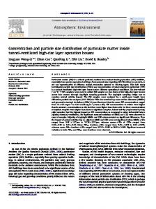
5 Comparison with the data of DNS/Lagrangian tracking For to compare the presented theory with the results of DNS/Lagrangian tracking of wall-bounded particle-laden turbulent flows we have to bear in mind that according to the considerations discussed in Sec. 3.6 the particle concentration in the vicinity of the wall can be smoothed due to unsteady effects. The estimate of the width of this region in Eq. (53) gives a value ∆y ∼ 0.4, which is relatively large, because the theory presented is valid only for small values of y, namely, y < y0 ≈ 3 ÷ 5 (see Sec. 3.3). The ratio ∆y/y0 seems to be on the edge of the validity range for the presented asymptotic theory, which can be applied if ∆y ≪ y < y0 holds. Unfortunately, according to Eq. (53) to improve the situation by reducing the ratio ∆y/y0 , say, to ten times one have to increase the simulation time of DNS/Lagrangian tracking to 100 times complicating thereby the computational efforts substantially. Below we will use for the comparison with theory the numerical data obtained in an international collaborative benchmark test of particle dispersion in the channel flow by different DNS codes presented in [41], where the computational time was Tsim = 2.1 · 104 . Particles in [41] were assumed to bounce the wall elastically, which corresponds to the case Jw = 0 in Eq. (46). Fig. 3 presents the profiles of particle concentration calculated by C.Marchioli and A.Soldati [41] with the pronounced near-wall peaks related with the accumulated particles for all three Stokes numbers τ = 1, 5, 25. As seen from Fig. 3, the power law for particle concentration profiles observed everywhere in the near-wall region y+ < 3 only for the most inertial particles with τ = 25, while the concentration profiles for particles with τ = 1, 5 are flattened in the region y+ < 1. As it was discussed in previous Section, this behavior is explained by the insufficient computational time to reach the steady statistics for particles with small Stokes numbers. This conclusion is also corroborated by Fig.5 from

24

Dmitrii Ph. Sikovsky

F/Fm

t 1 5 25

100

10

1

0.1

0.01 1

10

100

y

Fig. 3 Particle concentration across the channel for particle Stokes numbers τ = 1, 5, 25. Data of DNS/Lagrangian tracking simulation of C.Marchioli and A.Soldati [41]. Lines are the least-square fits of the numerical data in the range 1 < y < 3 (inside the rectangle).

[41]. It was shown in Sec. 3.4 that if Jw = 0, the leading term in Eq. (46) is the first one with power-law singularity, so that numerical data can be approximated by power-law fits. To extract the exponent α of power-law dependence −α Φ ∼ y+ we fitted all numerical data by straight lines in log-log plot using least-square fits in the range 1 < y+ < 3, where all numerical concentration profiles are almost linear in log-log coordinates (see this range highlighted by rectangle on Fig. 3). The same procedure was carried out for concentration profiles from the results of other contributors of the database [41] and the result is presented on Fig. 4. Power-law exponents extracted by the same way from the data of DNS/Lagrangian tracking [45] are also presented for comparison, though they had less computation time Tsim = 4000 and one should bear in mind that they are suffered from the influence of unsteady statistics much stronger than the data [41]. It is seen from Fig. 4 that the power exponents of near-wall concentration singularity show a clear trend of increasing with the Stokes number in spite of some tangible scatter. The reasons for such scatter between the data of different contributors are discussed in [41], where they are related mainly to the matter of the numerics, such as diverse numerical schemes, grid discretizations, interpolation techniques, the choice of the time-step size for particle tracking. In view of the complexity of numerical implementation of DNS/Lagrangian tracking method, the authors [41] believe this scatter to be acceptable. For the calculation of the analytical power-law exponent Eq. (44) we used the approximations Eq. (24). Then Eq. (44) becomes

α(τ ) =

4τ τ + TL

where the subscript ′ 0′ is omitted for brevity.

(55)

Singularity of inertial particle concentration in the viscous sublayer

25

a(t)

3

2 1 2 3 4 5 6

1

0 0

1

10

10

t

Fig. 4 Power exponent of the particle concentration singularity vs. particle relaxation time extracted from DNS/Lagrangian tracking numerical data of different contributors in the collaborative benchmark test [41] and [45]. Symbols: 1 - Marchioli and Soldati, 2 - Arcen and Tani` ere, 3 - Cargnelutti and Portela, 4 - Kuerten, 5 - Goldensoph and Squires (all from [41]), 6 - Chen, McLaughlin [45]. Curve is the expression Eq. (55)

The Lagrangian integral timescale of the fluid velocity seen by particle is taken from the model of Zaichik [15],[46] TL = {1 + 0.6875f (StE )}TLf , f (StE ) =

StE 0.45St2E − 1 + StE (1 + StE )2 (2 + StE )

(56)

where StE = (16/27)τ /TLf , TLf = 5 . From Fig. 4 it is seen the good agreement of the values of the power exponent calculated from Eqs. (55), (56) with those ones extracted from numerical data within their scatter. It is interesting to note that the good agreement is achieved with the help of a simple approximation for velocity autocorrelation function and the Lagrangian timescale model [46] developed for locally homogeneous isotropic turbulence. Fig. 5 presents the comparison of profiles of the flatness of wall-normal particle velocity and the particle concentration scaled by some factor for to superimpose these two distributions in a vicinity of the wall and to check the validity of Eq. (49) for n = 2

Fv =

⟨v 4 ⟩ ⟨v 2 ⟩

2

∼ Φ ∼ y −α ,

(57)

The singular behavior of the flatness predicted by the presented theory is clearly seen on Fig. 5. The corresponding profiles for τ = 1 are not presented here, because the particle statistics for this Stokes number did not reach the

26

Dmitrii Ph. Sikovsky

30F/Fm Fv,

48F/Fm Fv,

t=5

1000

100

100

10

10

1 1

10

t=25

1000

100

y

1 1

10

100

y

Fig. 5 Comparison of the profiles of the particle concentration and the flatness of the wallnormal particle velocity for Stokes number τ = 5 (left) and τ = 15 (right). Symbols are the numerical data C.Marchioli and A.Soldati [41]: black circles are the particle concentration scaled by the factor indicated on the title of vertical axis, white circles are the flatness of the particle velocity. Lines are the power-law least square fits for the concentration from Fig. 2.

steady state in the simulations [41] and the congruence of flatness and particle concentration profile is not yet developed. Since the numerical simulations [41] are made for the case χ = 1, the skewnesses of wall-normal velocity of particles are zero at the wall, as it was discussed above in Sec. 3.5.

6 Discussion and conclusions The method of matched asymptotic expansions has been applied to study the exact Kramers-Moyal equation Eq. (3) for the PDF of the normal velocity and the position of a point particle in the viscous sublayer of wall-bounded turbulent flow. It is shown that since the diffusion coefficients multiplying the higher derivatives in the Kramers-Moyal equation are goes to zero close to the wall, then the solution of this equation becomes singularly perturbed. The phase space are divided into the outer and inner layer with different solutions within each layer. The outer layer is occupied by the free-flight particles with large velocities thrown by large negative deviations of the fluid velocity from the core of the flow. Some of free-flight particles, which have no sufficient momentum to reach the wall, are stopping and decrease their velocities to the values comparable with small fluctuations of the near-wall fluid velocity and begin to move in statistical equilibrium with the fluid turbulent fluctuations. Such slow diffusional particles occupy the inner layer lying in the vicinity of the line v = 0 in the phase space and having the thickness decaying as y 2 . The Hilbert-class expansion Eq. (16) is constructed for the inner solution showing a singular behavior of the PDF at y → 0, which results in the power-law singularity of the particle concentration near the wall with the main contribution from the slow diffusional particles. The exact expression Eq. (44) for the leading exponent of the concentration power-law is obtained, which turned out to be a functional of the autocorrelation function of wall-normal fluid velocity seen by particle

Singularity of inertial particle concentration in the viscous sublayer

27

and the particle Stokes number only. The power-law singularities of the standardized moments of particle velocity such as the flatness, the skewness (in the case of the partial particle deposition χ ̸= 1) etc. at y → 0 are also shown. The predicted power-law exponents of near-wall singularities of the particle concentration and the particle velocity flatness are in good agreement with the corresponding exponents extracted from the data of numerical simulations of particle-laden turbulent flow in a plane channel. The singular behavior of PDF is the consequence of the point-particle approach, which is widely used for the modelling of particle-laden flows. The diffusional particles moving to the wall by turbophoresis are segregated until they touch the wall. The finite radius r of particles serves as the natural cut-off of the singularity at the distance y = r. Since the particle concentration singularity is formed by diffusional particles, which velocities are small and goes to zero at the wall, the build-up of the concentration profile with such singularity takes the infinite time. Thus, the finite time of observation (or simulation) plays the role of yet another regularizing factor smoothing the concentration profile at distances to the wall inversely proportional to the square root of observation time according to Eq. (53). This results is important for the proper choice of the simulation time in the Lagrangian tracking of particle-laden flows, in which the point-particle approach is used commonly and the finite radius of particles is taken into account by means of the boundary conditions at the wall [41]: the simulation time needed for to reach the steady-state statistics is inversely proportional to the square of the particle radius Eq. (52). In spite of the strong non-Gaussianity of wall-normal fluid velocity, the leading exponent Eq. (44) depends only on the second-order correlator of fluid velocity seen by particle, that is its value is the same for both Gaussian and non-Gaussian fields of the fluid velocity seen by particle. This might indicate good development perspectives for the Gaussian random walk models of particle dispersion, which appear to be able to simulate the near-wall particle concentration build-up at least qualitatively [11]. As for the continuum models of particulate phase, such as Eulerian two-fluid models, they cannot model this phenomenon even at a qualitative level, since, as is shown above, the particulate phase in a viscous sublayer is not a single continuum, but separates on two different groups of particles: free-flight and diffusional particles with strikingly different r.m.s. velocities. As a result at least the two-fluid description of particulate phase is needed in the continuum models. Wall singularity of the flatness of particle velocity resulting from ’free-flight-diffusional’ intermittency demonstrates the breakdown of the quasinormal closure assumption lying in the most second-moment closures for the particulate phase. The examples of non-physical behavior of the second-moment particle Reynolds stress models in wall-bounded turbulent flows can also be found in Chapter 2.6.1 of the book [15] and in [16]. The particle concentration singularity and the extreme intermittency of particle velocities seem necessary to take into account in further developments of the wall treatment for statistical models of turbulent particle-laden flows.

28

Dmitrii Ph. Sikovsky

Acknowledgements Work is supported by the grant of RF Government for Support of Scientific Research under the Direction of Leading Scientists in Russian Universities (No. 11.G34.31.0046, leading scientist Prof. Kemal Hanjalic, Novosibirsk State University) and by Program of Basic Research of the Energy, Engineering Industry, Mechanics and Control Processes of the Russian Academy of Sciences (No. 10-2). Author thanks Prof. Michael W. Reeks for the very useful and fruitful discussion. Author is grateful to anonymous referees for their penetrative and constructive comments. Author is cordially grateful to late Prof. Leonid Zaichik for inspiration.

References 1. Soldati, A., Marchioli, C. Physics and modelling of turbulent particle deposition and entrainment: Review of a systematic study. Int. J. Multiphase Flow, 35, 827-839 (2009). 2. Balachandar, S., Eaton, J.K.: Turbulent dispersed multiphase flows, Ann. Rev. Fluid Mech., 42, 111-133 (2010). 3. Reeks, M.W.: On a kinetic equation for the transport of particles in turbulent flows, Phys. Fluids A, 3, 446-456 (1991). 4. Zaichik, L.I.: A statistical model of particle transport and heat transfer in turbulent shear flows, Phys. Fluids, 11, 1521-1534 (1999). 5. Pozorski, J., Minier, J.-P.: Probability density function modeling of dispersed two-phase turbulent flows, Phys. Rev.E, 59, 855-863 (1999). 6. Derevich, I.V.: Statistical modelling of mass transfer in turbulent two-phase dispersed flows. I. Model development, Int. J. Heat Mass Transfer, 43, 3709-3723 (2000). 7. Simonin, O., Deutsch, E., Minier, J.P.: Eulerian prediction of fluid-particle correlated motion in turbulent two-phase flows, Appl. Sci. Res., 51, 275-283 (1993). 8. Minier, J.-P., Peirano, E.: The PDF approach to polydispersed turbulent two-phase flows, Physics Reports, 352, 1-214 (2001). 9. Chibbaro, S., Minier, J.-P.: Langevin PDF simulation of particle deposition in a turbulent pipe flow, J. Aerosol Sci., 39, 555-571 (2008). 10. Pope, S.B.: Lagrangian PDF methods for turbulent flows, Ann. Rev. Fluid Mech., 26, 23-63 (1994). 11. Arcen, B., Tani` ere, A.: Simulation of a particle-laden turbulent channel flow using an improved stochastic Lagrangian model, Phys. Fluids, 21, 043303 (2009). 12. Simonin, O.: Statistical and continuum modelling of turbulent reactive particulate flows. Part I: Theoretical derivation of dispersed phase Eulerian modelling from probability density function kinetic equation, von Karman Institute for Fluid Dynamics: Lecture Series, Belgium (2000). 13. Cercignani, C.: The Boltzmann equation and its application. Springer-Verlag, New York (1988) 14. Zaichik, L.I., Alipchenkov, V.M., Avetissian, A.R.: Transport and deposition of colliding particles in turbulent channel flows, Int. J. Heat Fluid Flow, 30, 443-451 (2009). 15. Zaichik, L.I., Alipchenkov, V.M., Sinaiski, E.G.: Particles in turbulent flows. Wiley-VCH Verlag, (2008). 16. Sikovsky, D.Ph.: Deposition of inertial particles from turbulent flow in channels at high Reynolds numbers, Thermophysics and Aeromechanics, 18, 235-254 (2011). 17. Tian, Z.F., Tu, J.Y., Yeoh, G.H.: Numerical simulation and validation of dilute gasparticle flow over a backward-facing step, Aerosol Sci. Tech., 39, 319-332 (2005). 18. Pakhomov, M.A., Terekhov, V.I.: Second-moment closure simulation of flow and heat transfer in a gas-droplets turbulent impinging jet, Int. J. Therm. Sci., 60, 1-12 (2012). 19. Kroshilin, A.E., Kukharenko, V.N., Nigmatulin, B.I.: Particle deposition on a channel wall in a turbulent disperse flow with gradient, Fluid Dynamics, 20, 542-547 (1985). 20. Swailes, D.C., Reeks, M.: Particle deposition from a turbulent flow. I: A steady-state model for high-inertia particles, Phys. Fluids, 6, 3392-3403 (1994). 21. van Dijk, P.J., Swailes, D.C.: Hermite-DG methods for pdf equations modelling particle transport and deposition in turbulent boundary layers, J. Comp. Phys., 231, 4904-4920 (2012).

Singularity of inertial particle concentration in the viscous sublayer

29

22. Lenaers, P., Li, Q., Brethouwer, G., Schlatter, P., Orlu, R.: Rare backflow and extreme wall-normal velocity fluctuations in near-wall turbulence. Phys. Fluids, 24, 035110 (2012). 23. Swailes, D.C., Darbyshire, K.F.F.: A generalized Fokker-Planck equation for particle transport in random media, Physica A, 242, 38-48 (1997). 24. Klyatskin, V.I.: Stochastic Equations through the Eye of the Physicist, 1st Edition. Elsevier, 2005. Chapter 5.4.1. 25. Reeks, M.W.: On the continuum equations for dispersed particles in nonuniform flows, Phys. Fluids A, 4, 1290-1303 (1992). 26. Piquet, J.: Turbulent Flows: Models and Physics. 2nd ed. Berlin: Springer (2001). 27. Oesterl´ e, B.,Zaichik, L.I.: On Lagrangian time scales and particle dispersion modeling in equilibrium turbulent shear flows, Phys. Fluids, 16, 3374-3384 (2004). 28. Shin, M. Kim, D.S., Lee, J.W.: Deposition of inertia-dominated particles inside a turbulent boundary layer, Int. J. Multiphase Flow, 29, 893-926 (2003). 29. Metzger, M.: Length and time scales of the near-surface axial velocity in a high Reynolds number turbulent boundary layer, Int. J. Heat Fluid Flow, 27, 534-541 (2006). 30. Metzger, M., McKeon, B., Arce-Larreta, E.: Length and time scales of the near-surface axial velocity in a high Reynolds number turbulent boundary layer, Physica D, 239, 12961304 (2010). 31. Robinson, S.K.: Coherent motions in the turbulent boundary layer, Ann. Rev. Fluid Mech., 23, 601-639 (1991). 32. Van Dyke, M.: Perturbation methods in fluid mechanics. Academic Press, New York (1964). 33. Tchen, C.M. Mean value and correlation problems connected with the motion of small particles suspended in a turbulent fluid. Ph.D. Thesis, Delft (1947). 34. Monin, A.S., Yaglom, A.M.: Statistical fluid mechanics. Vol. 1. Mechanics of Turbulence. M.I.T. Press, Cambridge, Mass. (1971). 35. Hoyas, S., Jimenez, J.: Reynolds number effects on the Reynolds-stress budgets in turbulent channels, Phys. Fluids, 20, 101511 (2008). 36. Garcia-Ybarra, P.L.: Near-wall turbulent transport of large-Schmidt-number passive scalars, Phys. Rev. E, 79, 067302 (2009). 37. Scalo, C., Piomelli, U., Boegman, L.: High-Schmidt-number mass transport mechanisms from a turbulent flow to absorbing sediments, Phys. Fluids, 24, 085103 (2012). 38. Smits, A.J., McKeon, B.J., Marusic, I.: High-Reynolds number wall turbulence, Ann. Rev. Fluid Mech., 43, 353-375 (2011). 39. Narayanan, C., Lakehal, D., Botto, L., Soldati, A.: Mechanism of the particle deposition in a fully developed turbulent open channel flow, Phys. Fluids, 15,763-775 (2003). 40. Burschka, M.A., Titulaer, U.M.: The kinetic boundary layer for the equation with absorbing boundary, J. Stat. Phys., 25, 569-582 (1981). 41. Marchioli, C., Soldati, A., Kuerten,J.G.M., Arcen, B., Taniere, A., Goldensoph, G., Squires, K.D., Cargnelutti, M.F., Portela, L.M.: Statistics of particle dispersion in direct numerical simulations of wall-bounded turbulence: Results of an international collaborative benchmark test, Int. J. Multiphase Flow, 34, 879-893 (2008). Datasets are downloaded from the web at http://cfd.cineca.it/cfd/repository/ 42. Gustavsson, K., Meneguz, E., Reeks, M., Mehlig, B.: Inertial-particle dynamics in turbulent flows: caustics, concentration fluctuations and random uncorrelated motion, New J. Phys., 14, 115017 (2012). 43. Gustavsson, K., Mehlig, B.: Distribution of relative velocities in turbulent aerosols, Phys. Rev. E, 84, 045304(R) (2011). 44. Gustavsson, K., Mehlig, B., Wilkinson, M., Uski, V.: Variable-Range Projection Model for Turbulence-Driven Collisions, Phys. Rev. Lett., 101, 174503 (2008). 45. Chen, M., McLaughlin, J.B.: A new correlation for the aerosol deposition rate in vertical ducts, J. Colloid and Interface Sci., 169, 437-455 (1995). 46. Oesterl´ e, B.,Zaichik, L.I.: Time scales for predicting dispersion of arbitrary-density particles in isotropic turbulence, Int. J. Multiphase Flow, 32, 838-849 (2006).