SITE INDEX: CONCEPTS AND METHODS OSCAR GARCIA Professor and Endowed Chair in Forest Growth and Yield University of Northern British Columbia, 3333 University Way, Prince George, BC, Canada V2N 4Z9,
[email protected]
Abstract Site index ideas are reviewed, stressing conceptual foundations and issues that are frequently misunderstood. The structure of site index models is explained first within a traditional deterministic context. When variability due to environmental fluctuations and observational errors is introduced, it is found that difficulties of procedure and interpretation appear. Overlooked differences in the definitions of site index implicitly used by various authors can cause confusion. The relationship between growth functions and differential equations is also examined. Rational parameter estimation requires a clear model for the error structure, and a general formulation is offered. The article ends with a brief review of several site modelling methods in terms of the concepts previously exposed.
1
Introduction
Site index models relate height, age and site quality (potential productivity) in even-aged single-species stands. They are used for predicting stand height development, and for assessing site quality. Various approaches are described in textbooks such as Belyea (1931), Spurr (1952), Clutter et al. (1983), and general reviews have been published by Jones (1969), Carmean (1975), H¨ agglund (1981), Ortega and Montero (1988), Grey (1989). In a deterministic setting, the ideas are relatively straightforward. However, when variability due to weather conditions and to sampling and/or measurement error is introduced, subtle pitfalls have caused confusion and controversy. Stochastic aspects are also important in devising and evaluating estimation procedures. What follows is an exposition of key issues, focusing on general concepts and estimation strategies.
2
Site index, deterministic
2.1 Basics. In order to reduce stand density effects, the height used in site index models is usually some measure based on the largest trees in a stand, such as the mean height of dominants and codominants or the average for a fixed number of largest trees per hectare. I shall refer to it as top height, or simply “height”. Age may be age from seed, age since planting, or age since reaching breast height. This last one, breast-height age, is sometimes easier to obtain and can eliminate variability in early stand development that is unrelated to site quality (Husch 1956). The basic site index idea is simple (Figure 1). Stands in better sites are supposed to follow height-age trajectories that are higher than those in poorer sites. Conceptually, there is an infinite number of curves, labeled by some parameter q. In symbols, H = f (t, q) ,
(1)
where H is top height and t is age (Bailey and Clutter 1974, H¨ agglund 1981). This is a 100
60
q5 q4
50
q3 q2
Top Height
40
q1
30
20
10
0 0
10
20
30
40 Age
50
60
70
80
Figure 1: Site curves, indexed by a site-dependent parameter q. one-parameter family of curves (James 1992, Kreyszig 1993)1 . Given a stand age and height, the site quality is assessed through the relative position of the curve that passes through that point. Conversely, for a given site quality, the corresponding curve predicts future stand height development. 2.2 Site index. Different site parameters q might be used. Clearly, any one-to-one transformation of q would serve equally well for identifying site quality. The most common labeling scheme uses a site index, defined as the curve height at a specified base age or index age (Figure 2). If S is site index and tb is the base age, the site index is related to any other q by substituting in (1): (2) S = f (tb , q) . It should be noted that the base age is essentially arbitrary, a conventional value used in labeling the site curves. 2.3 Local and global parameters. In specific models there are one or more other adjustable parameters (p1 , p2 , . . .) ≡ p. Therefore, we may write more fully: H = f (t, p, q) .
(3)
The pi are common to all stands or sample plots, while q is site-dependent, specific to each stand or plot. As shorthand, the site parameter q, which varies from place to place, has been 1 Alternatively, (1) could be seen as a surface where the site index curves are “slices” of constant q (e. g., Cieszewski 2002). However, the slices of constant t are less meaningful, and the family of curves interpretation seems simpler and more direct.
101
60
S5 S4
50
S3 S2
Top Height
40
S1
30
20
10
0 0
10
20
30
40 Age
50
60
70
80
Figure 2: Site index as curve labels. Base age 40. called “local”, and the pi , which stay the same over the whole population of stands, were called “global” (Garc´ıa 1983). 2.4
Examples. The Schumacher (1939) equation H = a exp(−b/t)
(4)
is often used in site index models. In “anamorphic” models, the site curves are vertically proportional. Therefore, in that case the proportionality constant a = q is the local parameter, and b is global. Alternatively, a site index S may be used as a local parameter instead of a. These parameters are related by S = a exp(−b/tb ), or a = S exp(b/tb ). Substituting in (4), H = S exp[−b(1/t − 1/tb )] .
(5)
Another popular height-age function is the Richards (von Bertalanffy 1949, Richards 1959), H = a[1 − exp(−bt)]c .
(6)
One so-called “polymorphic” (many shapes) version might have b = q as local, and a and c as globals (in fact, the curves are then horizontally proportional, with a common shape). The parameter b is related to S by S = a[1 − exp(−btb )]c , or b = − ln[1 − (S/a)1/c ]/tb . Substituting in (6) and simplifying, we obtain the model in terms of S: H = a{1 − [1 − (S/a)1/c ]t/tb }c .
(7)
More generally, (6), for instance, could be reparameterized: one might have a = a(q), b = b(q), c = c(q), with these functions involving other global parameters. Analytical solutions for a local parameter are not always available. 102
When applying a site index model, only estimates for the global parameters are needed. The site index or other local parameter selects a particular curve from the family, and it is not given any specific fixed value. 2.5 Base-age invariance. Bailey and Clutter (1974) introduced the idea of base-age invariance: because the choice of base age is arbitrary, it would be undesirable for a model to produce different results if different base ages are used. At least from an esthetical point of view. There are actually two forms of base-age invariance: 1. The equation form does not change when changing the base age. The examples above are base-age invariant, but there are many site index models in the literature where this is not the case. 2. The estimation procedure results in the same model no matter what base age (if any) is used in it.
3
Stochastics
3.1 Variability and definitions. So far, I have described height development in deterministic terms, ignoring variability over time and observational errors. In reality, differences in weather and other factors cause any particular stand to deviate from the expected trend. In addition, measurement and/or sampling error can make observations to differ from the real values (Figure 3)2 .
60
50
Top Height
40
30
20
10
0 0
10
20
30
40 Age
50
60
70
80
Figure 3: Actual stand height (continuous curve), and measurements (dots). 2 Measurement error can be substantial in permanent sample plots (PSPs), but may be small or negligible in stem-analysis data. On the other hand, stem analysis is prone to distortions from tree selection and changes of dominance, that can add to the actual height deviations.
103
Ignoring random variation is not necessarily bad in itself. A deterministic model may represent expected or most likely predictions. Often, this is all what a decision-maker wants, needs, and can use. Variability, however, can introduce interpretation and inference difficulties. The definition of site index was clear in the deterministic setting. Which or what is the site index in the situation described in Figure 3? Researchers appear to have adopted one of two positions: 1. Take literally the deterministic definition: site index is the height at base age. That is, the point corresponding to base age on the continuous curve of Figure 3. This is a property of the particular stand. We may call it “stand site index”. 2. More convoluted wording, trying to preserve the original concept of site index as a property of the site: an expected, average, or most likely height at base age. The point corresponding to base age on the dashed curve of Figure 3. Call it “site site index”. Definitions may be more or less natural, more or less useful, but they can not be wrong. However, failing to recognize implicit differences in meanings may have caused controversy and misunderstandings (e. g., Goelz and Burk 1992, Bailey and Cieszewski 2000, and references therein). I take a site site index view: “Site index is the most likely top height at a base age among all the hypothetical stands that could grow on the site”. Similarly, site curves and q are interpreted as most likely values. 3.2 Modelling. A second question relates to estimation. Devising rational estimation procedures requires having a reasonable stochastic model for the data error structure. I describe a very general formulation first. It is clear that the height deviations of a sample plot (or stand) from the expected trend are serially correlated: once the stand is on one side of the trend, more likely than not it will be on the same side in the future (Figure 3). To understand the stand trajectory, it is best to think of it as the accumulation or integration of height growth rates, either periodic, ∆H, or instantaneous, dH/dt. The choice between descriptions in discrete or in continuous time is often largely a question of personal taste. It is not usually expected for a continuous projection to make sense at scales below one year, unless some kind of “physiological time” that takes into account seasonal growth changes is used. On the other hand, finite increments can be generated from integration of instantaneous rates, ignoring the intra-annual detail if so desired, and tools for working with derivatives are more convenient and more highly developed than those for finite differences. This is one of those instances in mathematics where embedding a particular case (discrete time) into a more general class of problems (continuous time) makes it easier to handle3 . Therefore, let us model the growth rate dH/dt. In general, this rate is a function of the current height, and possibly age, and contains a local parameter and one or more global parameters. For the perturbations due to weather, etc., a random value u(t) is included, which belongs to some random process u representing “environmental noise”: dH = g(H, t, p, q, u(t)) dt
(8)
H(t0 ) = H0 . In the initial condition, t0 = H0 = 0 for curves through the origin, H0 = 1.3 at t0 = 0 when using breast-height age, or for added flexibility, t0 or H0 may be left as a free parameter to be estimated from the data. Equation (8) is a stochastic differential equation (SDE), since it includes a stochastic process u. Again, we do not need to go into the theory of SDEs, we just use some of the jargon. 3 Fortunately, little or no differential equation (DE) theory is usually needed. Most univariate DEs in forestry are separable. To solve, move all occurrences of the dependent variable to the left-hand side, all those of the independent variable to the right, and integrate both sides.
104
Our data consists of several observations h1 , h2 , . . . in each sample plot, taken at ages t1 , t2 , . . .. These measurements may contain measurement and/or sampling errors εi : hi = H(ti ) + εi .
(9)
It is necessary to estimate the parameters p, and perhaps t0 or H0 .
4
Estimation
I shall discuss briefly the principles behind three of the most commonly used site index model estimation methods, followed by an approach based on the stochastic structure just described. I assume that each sample plot has several observations, either from PSP remeasurement or from stem analysis. For methods appropriate when only single height-age pairs in temporary plots are available, see Walters et al. (1989). It is necessary to estimate the global parameters p, and to somehow handle also the local parameter qi associated with each plot. This makes for a very large number of parameters, requiring specialized methods. 4.1 Parameter prediction. This method (see e. g., Clutter et al. 1983) proceeds in two stages: 1. Consider all the parameters as locals. That is, fit separately the model to each plot. The local parameter qi is usually the site index. 2. Keep the qi , and re-estimate common values for the globals. This is commonly done by regressing each global parameter over qi , using the estimates from the first stage. In general, the site curves obtained do not pass through the site index at base age. Often the model is somehow adjusted to correct this, mostly cosmetic, defect. With the usual choice of S for q, the method is not base-age invariant. 4.2 Mixed effects. Recently, linear or nonlinear mixed-effects models have become popular in site index modelling (Lappi and Bailey 1988, Gregoire et al. 1995, Hall and Bailey 2001). Attractive features are that they are part of mainstream Statistics, and that they are easily accessible through standard statistical packages (for instance, Venables and Ripley 2002). These methods consider q as a random variable (random effect) that varies within a population of stands. Interest focuses on estimating fixed effects, here the global parameters. Serial correlation can be approximated by an autoregressive error process (Gregoire et al. 1995, Seber and Wild 2003). The theory assumes that q has a certain probability distribution in the population, and that the q in the sample correspond to the same distribution. That is, it is assumed that the sample plots constitute a simple random sample. This is rarely, if ever, the case in practice. 4.3 Growth functions and differential equations. To explain the third class of site index modelling methods, a digression into the relationship between growth curves and differential equations is needed. It is often incorrectly assumed that there is a unique differential equation (DE) associated with any (deterministic) growth function. Given a growth function (1) for a fixed q, possibly written with a transformation of H such as its logarithm, it is differentiated producing a DE dH = g(t, H, q) . dt
(10)
However, being at a point on the curve (Figure 4), it is possible to substitute (1) into the right-hand side of (10) to obtain a DE dH/dt = g1 (t, q) that does not contain H. Or t may 105
be eliminated between (1) and (10) to obtain a DE dH/dt = g2 (H, q) that has only H on the right-hand side (there are good physical and biological arguments to prefer this form). Or anything in-between; e. g., write H = H k H 1−k , and substitute in only one of the factors.
60
50 dH/dt
Top Height
40
30
20
10
0 0
10
20
30
40
50
60
70
80
Age Figure 4: Growth function and derivative. All these DEs are equivalent in the deterministic case, in that by integration they generate the same growth curve. Once we are off the curve, however, they differ. A particularly interesting alternative is to eliminate q between (1) and (10), to get dH = g3 (t, H) . dt
(11)
This conveniently gets rid of the local parameters, leaving only the few globals to be estimated. The idea is behind the Bailey-Clutter difference equation method described next. Of course, used away from the growth curve this DE does not make sense: it would imply that the growth rate is independent of site quality4 . 4.4 Difference equation. Although not usually presented this way, this method (Bailey and Clutter 1974, Clutter et al. 1983) can be seen as an application of the q-free DE (11). Integrate (11) between two consecutive measurements, e. g., after separation of variables. This gives a relationship between each measurement, the previous measurement, and the global parameters. The parameters can then be estimated by least-squares. As a simpler, although perhaps less instructive derivation of the same relationship (Clutter et al. 1983), solve (1) for q. Then, substitute the observations from one measurement occasion 4 This equation form is presented in textbooks as the DE of a family of curves (e. g., Kreyszig 1993), which might be slightly confusing. True, it describes or generates the family, but it should not be interpreted as a growth rate. A simple way of obtaining it, when feasible, is to solve (1) for q, differentiate, and re-arrange.
106
for t and H. Do the same for the following measurement. The two right-hand sides must be equal. Incidentally, the method name is somewhat of a misnomer, since it does not involve difference equations in the standard meaning of the term (a relationship between consecutive elements of a sequence). 4.5 SDE. The preceding estimation methods are relatively simple and convenient, and may (or may not) produce satisfactory results in practice. They do ignore the error structure, or use a rough approximation. I attempted to use a more realistic model of the error structure implied by the general SDE discussed before (Garc´ıa 1983, Rennolls 1995, Seber and Wild 2003). A simple model could be linear, with parameters a and b: dH = b(a − H) + noise . dt Much more flexibility is achieved by allowing a power transformation of H: dH c = b(ac − H c ) + σ w(t) ˙ . dt
(12)
Here c and σ are additional parameters to be estimated, and w˙ is the formal derivative of a Wiener stochastic process, also known as white noise or Brownian motion. The basic assumption in this “environmental noise” term is that non-overlapping time intervals are independent. Integration of the SDE (12) results in a Richards function like (6), plus an error term with the serial correlation and increasing variance that one might expect5 . In addition to the environmental variation, measurement/sampling error is modelled as hci = H c (ti ) + ηεi ,
(13)
where the εi are normal and independently distributed. In general, each of the parameters a, b, c, σ, and η can be either global, local, or fixed at a known value, possibly after re-parameterization. All the parameters are estimated simultaneously by Maximum Likelihood, using a customized optimization algorithm. Software for carrying-out the estimation has recently been made more flexible and easy to use, and is available from http://www.unbc.ca/forestry/forestgrowth/sde. This method has given good results in a number of studies. The advantages of better error structure modelling and efficient information utilization may be most important with scarce and poor quality data.
5
Summary and conclusions
Site index ideas are relatively simple in a deterministic setting. The models can be interpreted as families of curves, or height-age equations that contain global and local parameters. Site index is seen as a special instance of local parameter. Two forms of base-age invariance were identified. When considering the deviations of individual stands from the nominal height-age trajectories, conceptual and communication difficulties arise. Differences between “stand site index” and “site site index” views can cause confusion and unnecessary controversy. The nature of heightage variability can be described by a general stochastic differential equation, plus measurement and/or sampling error. Another source of confusion has been the non-uniqueness in the differential representation of growth functions. Contrary to a common misconception, there is an infinity of differential 5 Rennolls (1995) independently developed essentially the same model, but through the somewhat more involved Fokker-Plank partial differential approach instead of the more recent SDE formalism. Growth functions other than the Richards could be used: there is a two-parameter transformation that linearizes almost all the models used in forestry (http://web.unbc.ca/∼garcia/unpub/unigrow.pdf).
107
equations that integrate to the same growth function. Under deviations from the deterministic trend, however, they are not equally meaningful as representing growth rates. Three commonly used estimation procedures, and another approach based on the stochastic differential equation, were reviewed in light of the concepts previously exposed. It is felt that various methods can produce acceptable results with good quality data, but that efficient procedures based on more accurate modelling of error structures become critical in data-poor situations.
References Bailey, R. L. and Cieszewski, C. J. (2000). Development of a well-behaved site-index equation: jack pine in north-central Ontario: Comment. Can.J.For.Res., 30:1667–1668. Bailey, R. L. and Clutter, J. L. (1974). Base-age invariant polymorphic site curves. For.Sci., 20:155–159. Belyea, H. C. (1931). Forest Measurement. Wiley, New York. 302 p. Carmean, W. H. (1975). Forest site quality evaluation in the United States. In Brady, N. C., editor, Advances in Agronomy, Vol. 27, pages 209–269. Academic Press, New York. Cieszewski, C. J. (2002). Comparing fixed- and variable-base-age site equations having single versus multiple asymptotes. For.Sci., 48(1):7–23. Clutter, J. L., Fortson, J. C., Pienaar, L. V., Brister, G. H., and Bailey, R. L. (1983). Timber Management: A Quantitative Approach. Wiley, New York. 333 p. Garc´ıa, O. (1983). A stochastic differential equation model for the height growth of forest stands. Biometrics, 39:1059–1072. Goelz, J. C. G. and Burk, T. E. (1992). Development of a well-behaved site-index equation: jack pine in north central Ontario. Can.J.For.Res., 22:776–784. Gregoire, T. G., Schabenberger, O., and Barrett, J. P. (1995). Linear modelling of irregularly spaced, unbalanced, longitudinal data from permanent-plot measurements. Can.J.For.Res., 25:137–156. Grey, D. C. (1989). Site index — A review. South African Forestry Journal, (148):28–32. H¨ agglund, B. (1981). Evaluation of forest site productivity. Forestry Abstracts, 42:515–527. Hall, D. B. and Bailey, R. L. (2001). Modelling and prediction of forest growth variables based on multilevel nonlinear mixed models. For.Sci., 47:311–321. Husch, B. (1956). Use of age at dbh as a variable in the site index concept. J.For., 54:340. James, R. C. (1992). Mathematics Dictionary. Chapman & Hall, New York, Fifth edition. 548 p. Jones, J. R. (1969). Review and comparison of site evaluation methods. Research Paper RM-51, USDA Forest Service. 27 p. Kreyszig, E. (1993). Advanced Engineering Mathematics. Wiley, New York, Seventh edition. 1271 p. Lappi, J. and Bailey, R. L. (1988). A height prediction model with random stand and tree parameters: an alternative to traditional site index methods. For.Sci., 34:907–927. Ortega, A. and Montero, G. (1988). Evaluaci´on de la calidad de las estaciones forestales. Revisi´on bibliogr´ afica. Ecolog´ıa, 2:151–184. 108
Rennolls, K. (1995). Forest height growth modelling. Forest Ecology and Management, 71:217– 225. Richards, F. J. (1959). A flexible growth function for empirical use. Journal of Experimental Botany, 10:290–300. Schumacher, F. X. (1939). A new growth curve and its application to timber-yield studies. J.For., 37:819–820. Seber, G. A. F. and Wild, C. J. (2003). Nonlinear Regression. Wiley-Interscience, New York. 768 p. Spurr, S. H. (1952). Forest Inventory. Ronald Press, New York. 476 p. Venables, W. N. and Ripley, B. D. (2002). Modern Applied Statistics with S. Springer, New York, fourth edition. 495 p. von Bertalanffy, L. (1949). Problems of organic growth. Nature, 163:156–158. Walters, D. K., Gregoire, T. G., and Burkhart, H. E. (1989). Consistent estimation of site index curves fitted to temporary plot data. Biometrics, 45:23–33.
109