Size and Effort Estimation Techniques for Software Development

ISSN (Print): 2279-0063 ISSN (Online): 2279-0071

International Association of Scientific Innovation and Research (IASIR) (An Association Unifying the Sciences, Engineering, and Applied Research)

International Journal of Software and Web Sciences (IJSWS) www.iasir.net Size and Effort Estimation Techniques for Software Development 1

Chander Diwaker, 2Astha Dhiman, Faculty of Computer Sc. & Engineering, 2Research Scholar Department of Computer Science & Engineering, University Institute of Engineering & Technology, Kurukshetra University, Kurukshetra -136 119, Haryana, INDIA. 1

Abstract: Software development Cost estimation is process of predicting the most realistic use of cost required for developing software based on some parameters. The estimation of various project parameters that include project size, effort required to develop the software, project duration and cost. It has always the biggest challenges in computer science for last decades because cost and time estimate at the early stage are difficult to obtain and they are often least accurate. Nowadays software project managers should be aware about increasing of project failures. The main reason for project failure is imprecision in the estimation. Project managers stress on importance of improving estimation accuracy and methods to support better estimates. The researchers have examined several existing methods for software development cost estimation. Suitability of estimation methods depends on factors like software application domain, product complexity, availability of historical data, team expertise etc. Keywords: COCOMO; COCOMO II; Effort; Cost; Size; Function point Metric I.

Introduction

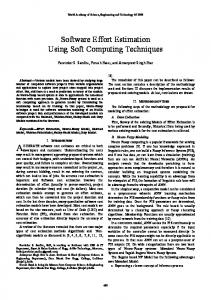
Software is expensive to develop and the major cost factor in corporate information systems budgets. Over the years, as hardware cost has reduced slowly, but cost of producing software has not changed significantly [1]. Software estimation process includes estimating the size of software product to be produced, estimating the effort needed, developing the preliminary project schedules, and finally estimating overall cost of the project. In last three decades, many software cost estimation methods have been developed including algorithmic methods, estimating by analogy, expert judgment method, price to win method, top-down method, and bottom-up method. These methods are not necessarily better or worse than other methods but their strengths and weaknesses are often complimentary to each other [2]. In this paper, we study various methods for development of Software cost Estimation. The next section discusses the Software Size Estimation Techniques. In section 3, we discussed effort estimation methods. We conclude in Section 4. II. Software Size Estimation Techniques Software size is one of the key cost drivers that affect the cost of software projects [3]. The project size defines the measurement of problem complexity in terms of effort and time required to develop the product. To accurately estimate the project size, some metric is defined in Figure 1 which can express the software size [4]. Metrics for software size estimation

LOC

FP

Feature point Metric

UCP

Object Points

Figure 1 Software Size Estimation Metrics Software Size Estimation Techniques are defined one by one below: 2.1 Line of Code (LOC): In LOC, the project size is estimated by counting the number of source instructions in the developed program, excluding comments and header lines. Exact LOC can only be obtained after the project has completed. It has some drawbacks. No accepted standard definition exists for LOC. It is very difficult to accurate estimate LOC in final product from problem specification. So, the LOC metric is of little use to project managers during project planning [4]. 2.2 Function Point (FP): It overcomes the problems of LOC [3]. Albrecht (1983) presented Function Point metric to measure the functionality of the project [9]. Instead of counting the LOCs of a developed solution for

IJSWS 13-134; © 2013, IJSWS All Rights Reserved

Page 36

Chander et al., International Journal of Software and Web Sciences, 4(1), March-May, 2013, pp. 36-40

the problem, it counts the size of the problem to solve [3]. The five user function types for which counts are made are divided into two categories [7]:  Data function Types: Internal Logical File (ILF) & External Interface Files (EIF). 

Transactional function types: External Input (EI), External Output (EO) & External Inquiry (EI).

Each instance of these above five function types is then classified by the complexity level. Complexity levels determine a set of weights, which are applied to their corresponding function counts to determine unadjusted function points (UFP) quantity. Classify each function count into Low, Average and High complexity levels depending on the number of data element types contained and the number of file types referenced. Table 1 shows the complexity rating matrix for the different categories calculated [8]. For ILF and EIF Record Elements

For EO and EQ

Data Elements 1-19

20-50

51+

Record Elements

For EI

Data Elements 1-5

6-19

20+

Record Elements

Data Elements 1-4

5-15

16+

1

low

low

avg

0-1

low

low

avg

0-1

low

low

avg

2-5

low

avg

high

2-3

low

avg

high

2-3

low

avg

high

6+

avg

high

high

4+

avg

high

high

4+

avg

high

high

Table 1 Function point complexity matrix [8] Apply the complexity weights as given in Table 2. The weight reflects relative value of the function to the user [8]. Function Type

Internal Logical Files External Interface Files External Inputs External Outputs External Inquiries

Complexity-Weight Low 7.0 5.0 3.0 4.0 3.0

Average 10.0 7.0 4.0 5.0 4.0

High 15.0 10.0 6.0 7.0 6.0

Table 2 Function Point Complexity Weight Metrics [8] The UFP is calculated by multiplying the complexity weights and the counts for each function component. Add all the weighted functions counts to get UFP [8]. In addition to the value of these components, 14 other software system characteristics are also considered in the measurement process. The sum of their rating scores is called Technical Complexity Factors (TCF) that expresses their influence on the overall complexity of the software system [1]. Each component can rated from 0 to 5 where 0 indicate that the component has no effect on the project and 5 means the component is compulsory and very important respectively [9]. Computation: According to paper [9], the TCF is calculated as: TCF = 0.65+0.01(SUM (Fi)) The TCF can range between 0.65 (if all Fi are 0) and 1.35 (if all Fi are 5). The final Function Point can be calculated as [9]: FP=UFC*TCF FP is not dependent on construction method [8]. Function points are independent of the language, tools or methodologies used for the implementation [2]. But the calculation of function points is complex and varies for different classes of software systems [8]. 2.3 Feature Point Metric: Feature Point metric extends the function points to include algorithms as a new class. Each algorithm used is given a weight range from 1 (elementary) to 10 (sophisticated algorithms). The feature point is weighted sum of the algorithms plus the function points. Another extension of the function points is Full Function Point (FFP) for measuring real-time applications [5]. 2.4 Use-Case Points (UCP): Use-Case Points method was developed by Gustav Karner of Objectory. Use-case Points are counted from the use-case analysis of system. UCP are counted during early phases of an objectoriented project that captures its scope with use cases. Each use-case is scaled as easy, medium, or hard to produce the point count. The use-case points can be also adjusted for project’s technical and personnel attributes, and directly converted to the hours in order to obtain a rough idea of a nominal project schedule [8]. 2.5 Object Points: While feature point and FFP extend function point, the object point measures the size from a different dimension.

IJSWS 13-134; © 2013, IJSWS All Rights Reserved

Page 37

Chander et al., International Journal of Software and Web Sciences, 4(1), March-May, 2013, pp. 36-40

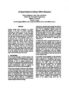
This measurement is based on the number and complexity of following objects i.e. screens, reports and 3GL components. This is relatively new measurement and not been yet very popular. But as it is easy to use at the early phase of the development cycle and also measures software size reasonably well so this measurement has been used in major estimation models such as COCOMO II for cost estimation [5]. III. Software Development Effort Estimation Techniques Software organizations are using various cost estimation models, techniques or methods to estimate the exact and accurate cost that will be used in the development of software project [3]. Figure 2 represents software development effort estimation methods. Software development effort estimation method

Expert based

Bottom-up

Top-down

Analogy based

SLIM

COCOMO I

COCOMO II

Figure 2 Software Development Effort Estimation Techniques 3.1 Expert Judgment Technique: Experts usually use their experience and understanding of a new project and available information about new and past projects to derive an estimate [3]. This is dependent on the ‘expert’ [5]. Another technique namely ‘Delphi approach’ tries to overcome some of the shortcoming of the Expert judgment approach. The coordinator prepares a summary of the responses from the experts on a form requesting another iteration of the experts’ estimates and the rationale for the estimates [5]. 3.2 Bottom-up Estimating Method: The cost of each software components is estimated and then combines the results to arrive at an estimated cost of overall project. It is more stable because estimation errors in the various components have a chance to balance out. But it is more time-consuming [2]. 3.3 Top-down Estimating Method: It is opposite of bottom-up method [5]. An overall cost estimation for project is derived from global properties of software project. Then project is partitioned into various low-level components. It is faster, easier to implement but not identify low-level problems [2]. 3.4 Analogy based Methods: It solves new problem by modifying solutions that were used to solve an old problem. The advantage of this method is that estimation is based on actual project characteristic data. Also Past experience and knowledge can be used which is not easy to be quantified [2]. 3.5 Software Life Cycle Management (SLIM) Method: Putnam developed a constraint model called SLIM that is applied to projects exceeding 70,000 lines of code. This model is very sensitive to development time as decreasing the development time can greatly increase the person months needed for development. The problem with this model is that it is based on knowing or being able to estimate accurately the size in lines of code of the software to be developed. There is great uncertainty in the software size. So it may result in inaccuracy of cost estimation [2]. 3.6 Constructive Cost Model (COCOMO I): This is one of the best-known and best-documented software effort estimation methods. It is the set of three modeling levels: Basic, Intermediate, and Detailed [3]. It has been experiencing difficulties in estimating the cost of software developed to new life cycle processes and capabilities including rapid-development process model, reuse-driven approaches and object-oriented approaches. For these reasons the newest version COCOMOІІ was developed [2]. 3.7 COCOMO ІІ: The capabilities of COCOMO II are size measurement in KLOC, Function Points, or Object Points. COCOMO II adjusts for software reuse and reengineering. This new model served as a framework for an extensive current data collection and analysis effort to further refine and calibrate the model's estimation capabilities [2]. This model has three sub-models defined below [8]: 3.7.1 Application Composition Model: involves prototyping efforts to resolve potential high-risk issues like as user interfaces, software/system interaction, performance, or technology maturity. It uses object points for sizing. 3.7.2 Early Design Model: involves exploration of alternative software/system architectures. It involves use of function points for sizing and a small number of additional cost drivers. 3.7.3 Post-Architecture (PA) Model: involves actual development and maintenance of a software product. It uses source instructions and/or function points for sizing, with modifiers for reuse and software breakage [8]. According to paper [8], COCOMO II method calculates the software development effort (in person months) by using the following equation: Effort = A × (SIZE) E × Πi EMi. Where, A- multiplicative constant with value 2.94 that scales the effort according to specific project conditions.

IJSWS 13-134; © 2013, IJSWS All Rights Reserved

Page 38

Chander et al., International Journal of Software and Web Sciences, 4(1), March-May, 2013, pp. 36-40

Size - Estimated size of a project in Kilo Source Lines of Code or Unadjusted Function Points. E - An exponential factor that accounts for the relative economies or diseconomies of scale encountered as a software project increases its size. EMi - Effort Multipliers. This model uses 17 Effort Multipliers (EMs) [8].Table 3 summarizes COCOMO II effort multipliers cost drivers by the categories of Product, Computer, Personnel and Project factors [10]. Cost Drivers

Description

Type

RELY

Required software reliability

Product

DATA

Data base Size

Product

RUSE

Developed for Reusability

Product

DOCU

Documentation needs

Product

CPLX

Product complexity

Product

TIME

Execution Time Constraints

Computer

STOR

Main Storage Constraints

Computer

PVOL

Platform Volatility

Computer

ACAP

Analyst Capability

Personnel

PCAP

Programmer Capability

Personnel

AEXP

Application Experience

Personnel

PEXP

Platform Experience

Personnel

LTEX

Language ad tool experience

Personnel

PCON

Personnel Continuity

Project

TOOL

Use of Software Tools

Project

SITE

Multi site Development

Project

SCED

Required Development Schedule

Project

Table 3 Cost driver for COCOMO-II PA model [10] The coefficient E is determined by weighing the predefined scale factors (SFi) and summing them using following equation [8]: E = 0.91 + 0.01 ∑i SFi The development time (TDEV) is derived from the effort according to the following equation [8]: TDEV = C × (Effort) F Latest calibration of the method shows that the multiplier C is equal to 3.67 and the coefficient F is determined is a similar way as the scale exponent by using following equation [8]: F = 0.28 + 0.002 ∑i SFi According to paper [8], when all the factors and multipliers are taken with their nominal values, then the equations for effort and schedule are given as follows: Effort = 2.94 × (Size) 1.1 Duration: TDEV = 3.67 × (Effort) 3.18 COCOMOII is clear and effective calibration process by combining Delphi technique with algorithmic cost estimation techniques. It is tool supportive and objective [6]. This model is repeatable, versatile [8]. But its limitation is that most of extensions are still experimental and not fully calibrated till now [6]. IV. Conclusion In this paper, an overview of software estimation techniques classifying them in broad categories. The strengths and weaknesses of these approaches have been discussed. The ideal size estimation method would define a relatively simple metric directly related to product size, would not depend on chosen construction technology and could be applied starting early in the project life-cycle. For known projects, we should use the expert judgment method or analogy method if the similarities of them can be got, since it is fast and reliable. For large and lesser known projects, it is better to use algorithmic model like COCOMO II. It is served as a framework for an extensive current data collection and analysis effort to further refine and calibrate the model's estimation capabilities. It provides the accurate result because more variables are considered including reuse parameter. This parameter is one of the essential variables in estimating the cost in the web-based application development. The search for reliable, accurate and the low cost estimation methods must continue. Trying to improve the performance of existing methods and introducing new methods for estimation based on today’s software project requirements can be the future works in this area. References [1] Xiangzhu gao and Bruce Lo, “An Integrated Software Cost Model Based on COCOMO and Function Point Approaches” Southern Cross University, In 1995 IEEE, pp. 86-88 IJSWS 13-134; © 2013, IJSWS All Rights Reserved

Page 39

Chander et al., International Journal of Software and Web Sciences, 4(1), March-May, 2013, pp. 36-40

[2] Liming Wu, “The Comparison of the Software Cost Estimating Methods” University of Calgary, pp. 2-12 [3] Lionel C. Briand, Isabella Wieczorek, “Resource Estimation in Software Engineering” In the second edition of the Encyclopedia of Software Engineering, 2001, pp. 1-52 [4] Rajib Mall, “Fundamentals of Software Engineering” pp. 38-53 [5] Hareton Leung, Zhang Fan, “Software cost estimation” Department of Computing, The Hong Kong Polytechnic University, pp. 2-12 [6] Nancy Merlo–Schett, “Seminar on Software Cost Estimation” WS 2002/2003, Department of Computer Science, pp. 3-19 [7] K. K. Aggarwal, Yogesh Singh, “ Software Engineering” 3rd Edition, pp. 143-179 [8] Bogdan Stępień “Software Development Cost Estimation Methods and Research Trends” Computer Science, Vol. 5, 2003, pp. 68-82 [9] Vahid Khatibi, Dayang N. A. Jawawi, “Software Cost Estimation Methods: A Review” Vol. 2, no. 1, ISSN 2079-8407, pp. 22-24 [10] Taeho Lee, Donoh Choi, Jongmoon Baik, “Empirical Study on Enhancing the Accuracy of Software Cost Estimation Model for Defense Software Development Project Applications” ISBN 978-89-5519-146-2, 2010 ICACT, pp.1117-1119.

IJSWS 13-134; © 2013, IJSWS All Rights Reserved

Page 40