SLAC-PUB-4531 January 25, 1988 T
SIZE AND SHAPE OF STRINGS*
M. KARLINER
and
I. KLEBANOV
Stanford Linear Accelerator Stanford
University,
Stanford,
Center
California,
94305
and
L. SIJSSKIND t Physics Department Stanford Stanford,
University
California
94305
ABSTRACT We study numerically of a fundamental and have divergent
and analytically
string in the light-cone
spatial properties
gauge. We find that strings are smooth
average size. Their properties
expected from particles
Submitted
in a conventional
to International
of the ground state
are very different
from what is
field theory.
Journal
of Modern
Physics A
* Work supported by the Department of Energy, contract DE-AC03-76SFOO515. f Work supported by NSF PHY 812280
1. Introduction String
theory was originally
idealized
mathematical
couple strings
invented
to describe hadrons[l].
theory. of hadrons failed,
to the external
Ultimately
due in part to the inability
local fields, such as the electromagnetic
reason for this failure is the infinity
field.
of normal mode zero point fluctuations
this to The
spread-
ing the string over all space[2]. In this paper we will examine in detail the spatial properties
of fundamental
strings.
We will also speculate
on how they compare
with the strings of large-N,,l,,
gauge theory[3].
in the following
of the ground state of the fundamental
characteristics
W e will be particularly
interested string:
1. The average size of the spatial region occupied by the string; 2. The average length of the string; 3. Is the string smooth on small scales or does it exhibit
rough or fractal-like
behaviour? 4. How densely is space filled with string? In order to answer these questions constructed
a numerical
the string.
and to provide
method for generating
gauge to generate a statistical
the overwhelming
majority
ensemble of strings.
of the ensemble have similar
‘snapshots’ are shown in section 2 and their important particular
of free string in the In fact we find that
qualitative
features.
The
features are discussed.
In
we find that both the average length of string and the average size of
the region occupied divergences
by the string are infinite.
is such that
that the string
string
actually
is microscopically
The relationship
between the two
packs the space densely.
very smooth,
on small scales. The quantitative
be provided
with
no tendency
We also find to form fractal
meaning of the above statements
will
later.
In section 3 some analytic findings
we have
‘snapshots’ of the ground state of
For that purpose we use the exact wave function
light-cone
structure
some intuition
derivations
are given to substantiate
of section 2. In section 4 we explain 2
the physical
the qualitative
meaning and measura-
bility
of the divergence in the size of the string.
qualitative N
COlOT
differences
We also speculate on the possible
between the fundamental
strings
and the strings
of large-
&CD.
2. Snapshots of Strings In the light-cone
gauge, the transverse
coordinates
of the string are free fields
with mode expansions
X”(o)
= XE, + x(X:
cos(na) + iQ sin(n0))
(24
n>O
The wave function has the product
for each transverse
form (dropping
coordinate
the superscript
in the ground state of the string i)
+ X:)/4)) Q(X(4) = n ( cp2 eXp(-Wn(X,2 n with
wn = n.
position
Squaring
of the string.
mode expansion introducing limit
distribution
To carry this out in practice
at some maximum
a cut-off in the parameter
wave number
for the transverse
it is necessary to truncate N.
the
This is one of the ways of
space of the string.
Passage to the continuum
is achieved as N + 00. Another
cut-off
procedure
discrete mass points that
this gives a probability
P-2)
the positions
connected
can be defined where string is replaced by 2N + 1 by identical
of the mass points
values of the parameter the string wave function
IY = 27rm/(2N
springs.
The normal
modes are such
are given by eq.(2.1) evaluated
at discrete
+ l), w 1rere m labels the mass points.
Then
is eq. (2.2) with frequencies
W n=
2N+l 7r
sin(
where n = 1, . . . , N. 3
7m 2N+l
>,
(2.3)
With
both cut-off
prescriptions
a string
configuration
quenceofvaluesofXiandXd,withn=l,
is determined
. . . . Nandi=l,
by a se-
. . . . D-2,sampled
with probability P(XA) and similarly
procedure
curve in (D - 2)-d imensional 2 transverse
dimensions.
each such configuration
compute
curves with
following
method:
In practice
as we proceed,
of string onto
each run consists of choosing 100 probability
distributions.
for example,
from
x
(D - 2)
For each run we
N = 10, 20, 30, 40, 50. F or convenience,
let us adopt the
N = 10 to N
= 20, the
of the normal modes with the first 10 wave numbers are kept the same
as for the N = 10 ‘snapshot’. to 50, always retaining increasing
defines a parametrized
space. By necessity we show projection
numbers from their respective
coefficients
(2.4)
eXP(-Wn(XA)2/2)
for Xi.
For the first cut-off
random
= (y2
Similarly,
the previous
N corresponds
we proceed from N = 20 to 30 to 40
set of coefficients.
to observing
Therefore,
for each run,
the same string with improved
resolution.
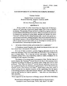
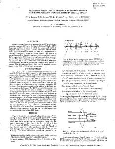
The ‘snapshots’ generated by 2 such runs are shown in figure 1 and figure 2. For one of the runs we also show graphs of total average transverse show curvature
line curvature
as a function
We find the following
transverse
( figure 4 ) as a function
length
( figure 3 ) and
of N.
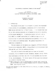
In figure 5 we
of length along the string for cases with N = 10, 20.
qualitative
features:
1. Slow growth of the occupied region with N. In the next section we will show that the growth
is actually
logarithmic.
2. The plots of total string length vs. N appear to be linear. we will show an analytic 3. The transverse mately
curvature
independent
derivation
of this effect.
averaged over the string
of the cut-off.
ically that the expectation
In the next section
appears to be approxi-
In the next section we will show analyt-
value of curvature
dent. 4
is completely
cut-off
indepen-
4. The growth
in length with increasing
smooth structures. similar
N is achieved by repetition
of similar
In fact, a piece of string of given length at N = 20 looks
to a piece of the same length at N = 10, (cf. Fig. 5).
5. The slow growth
of the occupied volume together
with the linear growth
of
length means that there is a strong tendency for the string to pass through the same small region many times. the string fills space densely:
It is obvious that,
as the cut-off
there is a point on the string
is removed,
arbitrarily
close
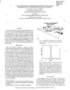
to any point in space. In order to elaborate
on point
(4) and show that no ‘accidents’ occur as we
proceed to high values of the cut-off confined
between
remarkable
between the two can be qualitatively
invariance
is important
regarded as a statement
of the string.
except for (3), can also be observed with In figure 7 we show a typical
picture
at N = 50. It
in space. In section 3 we show that,
the average distance in space between each pair of neighboring This, of course, is responsible for the linear growth
Thus, all the important obtained
the discrete
to note that, as more and more discrete points crowd the a-axis, the
string never becomes continuous
a constant.
of the string
in our approach.
All the above features, regularization
the section
cr = 0 and 47r/N for N = 20 and N = 500 ( figure 6 ). The
similarity
of conformal
we have plotted
information
in the regularization
as N + 00,
points approaches of the total length.
about the spatial properties
of string can be
where the string never becomes continuous
This fact will be essential for treatment
of strings in discretized
5
space.
in space.
3. Analytical In this section
we give analytic
reached in the previous occupied
by the string
section. with
Results
derivations
of some qualitative
Let us begin with
the cut-off
N.
the growth
conclusions of the volume
Define r to be the rms distance of a
point on the string to its center of mass:
r2 = ((J?(g)
(3.1)
- 2c,)2)
Since there is no preferred point on the closed string, we can arbitrarily
r2 = (D-2) ( It follows
that
+-2)&x3
(5X,)” >
n=l
the rms volume
set r~ = 0.
= (n-2)5;
of the transverse
(3.2) n=l
n=l
region occupied
by string
-
(log N) 9. -To find the dependence of average length on the cut-off,
we start with
27r
(L) = / (4 da,
(3-3)
0
where
(3.4) By translation
invariance
in CT (L) = 27r (?I(0 = 0))
For each transverse
(3.5)
direction
WY Using
the fact
that
each x’:, is gaussian 6
distributed,
it is easy to show that
dXi/da(o
= 0) 1s ’ g aussian distributed
p.
=
with variance
5
n
=
n’(N2+
(3.7)
1).
1
Therefore,
v’= dx’/da
is distributed
according
to
(3.8)
P(C) - exp
As a result, the distribution
for the length of v’is
(3.9)
.D-3d,
It follows that
(4 =
Jam exp(-v2/2C2)uD-2dv Jam exp( -v2/2C2)vD-3dv
The slope of the linear growth determined sionality.
For example,
- c
N N
(3.10)
by above expression depends on dimen-
if the number of transverse
dimensions
is an even number
(D - 2 = 2x7) then (3.10) yields
w = 4”-1(21c((k- 1’-!a3’l)!)22 In particular,
(N + l/2 + 0(1/N))
(3.11)
in D = 26 we find
(L) x 21.54 (N + l/2)
(3.12)
As shown in figure 3, the data for any given run agrees well with this linear dependence. This shows that the standard length.
deviation
is small compared with the average
It is also interesting dimensions. growth
to study eqn.
Using the Stirling
of transverse
formula
(3.11) in the limit for the factorial
x m/m3
we find that the slope of
+ 0(1/d=)
as D becomes large. In D = 26 this predicts to the exact number
replaced
of
length with N is given by
(L) IN
Similar
of a large number
analytic
(3.13)
the slope of 21.76, which is very close
(3.12). results
by a collection
can be derived
of mass points
in the regularization
connected
by springs.
where string For example,
is the
length is Ld = c where the subscript
lqn+1)
labels the mass points.
Using translation
Wd)= w + 1)
(lLq2,
After
(3.14)
- qn,l invariance,
- &,I)
a few steps analogous to the ones for the continuous
(3.15)
regularization
we find
(L d ) = (2k - 1)
[email protected])1’2 (N + l/2 + 0(1/N)) 49k - 1)!)2 Note that,
with
the definition
discrete regularization ization.
However,
physical
conclusions
Extrinsic
of length
differs slightly
the linearity
(3.16)
(3.14), the slope of linear growth
from (3.11) f ound in the continuous
of growth
and other properties
important
in the regularfor our
are unaffected.
curvature
string is kept continuous.
can only be investigated It is conveniently
in the regularization
where the
expressed as
(3.17)
8
where 21 is the component
of a’= d2k/do2
normal to v’= dJ?/dg.
%(o = 0)= - &xi,
Since
(3.18)
n=l
eq. (3.6) implies that a’and v’are uncorrelated.
Therefore,
(4 = WLI) ($) .
From the distribution
(3.19)
(3.9) we find
(> 1
1 = a@ - 1)X2
.2
It is important (IZll)
to note that this diverges in D = 4. Since a’and 5 are not correlated,
is effectively
Denoting
(3.20)
IZll
the average length
of the vector
= a we find the probability
(3.18) in D - 3 dimensions.
distribution
a2 P(a) - exp(-T)aDm4da 2s
(3.21)
with
C2=en3 =($N(N + 1))" = c4
(3.22)
1
It follows that (K) - g/C2
is independent
of the cut-off!
After
a short calculation
we find (~) = ((k - 2)!)222k-3 (2k - 3)!& -
(3.23)
’
which in D = 26 yields (rc) = 0.216. This is in good agreement with figure 4 which shows the data for a sample run. In the limit of large dimensionality
(3.23) reduces
to
-& This confirms
the intuitive
expectation
(3.24) that increasing
string smoother. 9
dimensionality
makes the
On the lower end of the range of dimensionalities in D = 4, (cf.- Eq,
We b e1ieve there is a simple
(3.20)).
a kink,
where the tangent
From eq. (3.17) we see that at a kink the curvature
function)
singularity,
of projections
.
while at a cusp it has a non-integrable
of strings onto 2 transverse dimensions
likely 10 occur there. configurations high likelihood
reason for points
Therefore,
has an integrable singularity.
indicate
(S-
Our study
that cusps are fairly
we conjecture
of cusps in D = 4 is responsible
which
turns back onto
We find that most of these cusps are projections
in higher dimensions.
diverges
vector dJ?/dcr is discontinuous,
In other words, at a cusp string
and a cusp, where it vanishes. itself.
intuitive
There are two kinds of singular
this which we proceed to explain. can occur on a string:
the average curvature
that
of smooth
the relatively
for the divergence
in the average
curvature.
4. Discussion One may wonder whether sections are observable.
any of the strange effects described
In particular,
the infinite
rms radius seems very unphysical.
However, it does lead to an observable effect. Consider scattering string from a string at rest. The interaction light-cone
a number particle -
is mediated
Oscillations
with frequency
of modes N E.
This introduces
radius
,/ii.
-
> l/r
This phenomenon
leads to the well-known
sections satisfied
by the dual amplitudes.[2]
and presents no obvious difficulty
In the
of the interaction
is of
average to zero. Thus, we retain
mode cut-off
As the resolution
of a high-energy
by string exchange.
frame of the fast string of energy E the lifetime
order r = l/E.
in the previous
and gives an observable
is improved,
the string
Regge behaviour
‘expands’.
of scattering
cross-
Th us the effect is indeed observable
for scattering
of strings by strings.
On the other hand, imagine that the string is being scattered by a local external field.
This situation
is analogous to the electromagnetic
this case the interaction infinite.
It is precisely
is instantaneous
and therefore
for this reason that 10
probing the string
the fundamental
of hadrons. must
strings
In
appear
cannot
be
consistently
coupled
theory of everything
to arbitrary
smooth.
fields.
That
is why they are either
a
or of nothing.
Let us speculate large-N,,l,,
external
now on how the fundamental
QCD strings.
Our results indicate
This should be contrasted 00 Migdal
strings
that
might
the fundamental
with the expected behaviour
In the limit
NcOlor +
and Makeenko
equation[3].
If QCD had an ultraviolet
croscopically
self-similar.
derived
fixed point
differ from the are
of QCD strings.
an exact lattice
then the string
QCD being asymptotically
strings
string
would be mi-
free is likely to make strings
even rougher. Another
difference between the QCD and fundamental
tial distribution measured facto]
of the longitudinal
by interaction
F(q2).
with
momentum
external
F or a fundamental
string
field.
an analogous
this could be
The result
form
factor
is a form can be ob-
of p+ is measured by the vertex operator
exp(iq . X), where (Y is the world sheet index.
&X+d”X+
In the light-cone
gauge
= T and the form factor reduces to F(q2> =
In the limit
N +
(J
only to the ground
- exp( -q2 log N)
da exp(iq +X(a))
is non-vanishing
x).
state of the string but also to any finitely
number
of normal
The strange behaviour
nected with
only at q = 0. It follows
all over space. This peculiar
any such state the change in the wave function cerns only a finite
the existence
relative
of the gravitational
of the graviton:
[4] states that in a Lorentz
energy-momentum
property
applies not
excited
state conin the limit
form factors is possibly
A theorem
con-
theory with
by Weinberg
a Lorentz
invariant
form factor of a massless spin-2 particle
must satisfy F(q2 # 0) = 0. It seems that string theory uses its infinite fluctuations
For
at least for the massless spin-2 state
invariant
tensor the gravitational
state.
to the ground
modes and becomes negligible
it could be foreseen on the basis of general principles. and Witten
(4.1)
>
00 the form factor
that p+ is smeared uniformly
N +
For a hadron,
gravitational
tained by observing that the distribution
X+
p +.
strings involves the spa-
to allow the existence of gravitons. 11
zero point
Acknowledgements:
We thank Marvin
Weinstein
for his help at the early stages of
this work.
.REFERENCES 1. For a review, see M. Green, J. Schwartz and E. Witten, Cambridge
Superstring
Theory,
U. Press, 1986.
2. L. Susskind,
Phys. Rev. Dl
(1970), 1182.
3. For a review, see A. A. Migdal, 4. S. Weinberg
and E. Witten,
Phys. Rep. 102 (1983), 199.
Phys. Lett. B96
FIGURE - 1) (a>+> P ro’Jec t ion
(1980), 59.
CAPTIONS
of string onto 2 transverse
dimensions
with
mode cut-off
N = 10, 20, 30, 40, 50. 2) Another
run, analogous to fig. 1.
3) Total transverse
length vs. mode cut-off for one run in D = 26. Broken line
shows the analytic 4) Transverse extrinsic
result for the expectation curvature
value, Eq. (3.11).
averaged over the string
one run in D = 26. Broken line shows the analytic
vs. mode cut-off for
result for the expectation
value, Eq. (3.22). 5) Transverse extrinsic
curvature
as a function
of length along the string for (a)
N = 10 and (b) N = 20. 6) Section of string confined between r~ = 0 and 47r/N for N = 20 (solid line) and N = 500 (dashed line). 7) A typical
configuration
of the ground state of 101 mass points connected by
springs.
12
FIG.
l(h)
x”
FIG.
l(B)
5
-
0
-
-5
-
,
1
1
-5
0
5
Xl
”
N max=30
5 -
0 -
FIG.
l(C)
-51 -5
0
5
1 ....I. 0
5
Xl
5 -
0 ??
-5 -
I FIG.
l(D)
I -5
Xl
N max=50
FIG.
l(E)
-5
0
5
Xl
FIG.
2(A)
-5
0 Xl
5
0-
-5-
FIG.
I
.
-5
2(B)
"
1'.
0
5
Xl
r
.
I
’
.
.
1
.
.
5 -
x”
0 -
-5-
I..“’
FIG.
2(C)
I.
” 0
-5 Xl
I 5
I
FIG.
2(D)
0
-5
5
Xl
FIG.
2(E)
I .,,,...,....I..1 0
-5
Xl
5
LENGTH VS CUTOFF
600
c 2 2 3 3
600
400
200 20
10
30
40
N FIG. 3
FIG.
3
AVE CURV VS CUTOFF
0.25 .-.-.-.-.-.-.-.-
_._._._.-.-.-.-.-. 0.20
.
0.15
0.10
0.05
0.00
10
30
20 N
FIG.
4
40
Curvature
vs length,
D=24,
N,,,
= 10
0.6 r
0.5
0.4
0.3
0.2
300
200
400
500
length
FIG.
Curvature
vs length,
5(A)
D=24,
N,,,
= 20
0.6
0.5
0.4
0
100
300
200 length
FIG.
5(B)
400
500
NMAX =20,500
N=ZO - ..-
N=500
\ .-./
Xl FIG.
6
NMAX =50
5 -
0 -
-5 -
-5
FIG.
7
0 Xl
5