Sketch Based Interfaces: Early Processing for Sketch Understanding Tevfik Metin Sezgin
Thomas Stahovich
Randall Davis
MIT AI Laboratory Massachusetts Institute of Technology Cambridge MA 02139, USA
CMU Deptarment of Mechanical Engineering Pittsburgh, PA 15213
MIT AI Laboratory Massachusetts Institute of Technology Cambridge MA 02139, USA
[email protected]
[email protected]
ABSTRACT
up having to sacrifice the utility of freehand sketching for the capabilities provided by the tools. When they move to a computer for detailed design, designers usually leave the sketch behind and the effort put into defining the rough geometry on paper is largely lost. We are working to provide a system where users can sketch naturally and have the sketches understood. By “understood” we mean that sketches can be used to convey to the system the same sorts of information about structure and behavior as they communicate to a human engineer. Such a system would allow users to interact with the computer without having to deal with icons, menus and tool selection, and would exploit direct manipulation (e.g., specifying curves by sketching them directly, rather than by specifying end points and control points). We also want users to be able to draw in an unrestricted fashion. It should, for example, be possible to draw a rectangle clockwise or counterclockwise, or with multiple strokes. Even more generally, the system, like people, should respond to how an object looks (e.g., like a rectangle), not how it was drawn. This will, we believe, produce a sketching interface that feels much more natural, unlike Graffiti and other gesture-based systems (e.g., [9], [14]), where pre-specified motions (e.g., an L-shaped stroke or a clockwise rectangular stroke) are required to specify a rectangular shape. The work reported here is part of our larger effort aimed at providing natural interaction with software, and with design tools in particular. That larger effort seeks to enable user to interact with automated tools in much the same manner as they interact with each other: by informal, messy sketches, verbal descriptions, and gestures. Our overall system uses a blackboard-style architecture [6], combining multiple sources of knowledge to produce a hierarchy of successively more abstract interpretations of a sketch. Our focus in this paper is on the very first step in the sketch understanding part of that larger undertaking: interpreting the pixels produced by the user’s strokes and producing low level geometric descriptions such as lines, ovals, rectangles, arbitrary polylines, curves and their combinations. Conversion from pixels to geometric objects is the first step in interpreting the input sketch. It provides a more compact representation and sets the stage for further, more abstract interpretation (e.g., interpreting a jagged line as a symbol for a spring).
Freehand sketching is a natural and crucial part of everyday human interaction, yet is almost totally unsupported by current user interfaces. We are working to combine the flexibility and ease of use of paper and pencil with the processing power of a computer, to produce a user interface for design that feels as natural as paper, yet is considerably smarter. One of the most basic steps in accomplishing this is converting the original digitized pen strokes in a sketch into the intended geometric objects. In this paper we describe an implemented system that combines multiple sources of knowledge to provide robust early processing for freehand sketching.
Categories and Subject Descriptors D.2.2 [Design Tools and Techniques]: User interfaces; H.5.2 [User Interfaces]: Input Devices and strategies; J.6 [Computer Aided Engineering]: CAD
General Terms Design, Human Factors
Keywords freehand sketching, natural interaction, multiple sources of knowledge
1.
[email protected]
INTRODUCTION
Freehand sketching is a familiar, efficient, and natural way of expressing certain kinds of ideas, particularly in the early phases of design. Yet this archetypal behavior is largely unsupported by user interfaces in general and by design software in particular, which has for the most part aimed at providing services in the later phases of design. As a result designers either forgo tool use at the early stage or end
Permission to make digital or hard copies of all or part of this work for personal or classroom use is granted without fee provided that copies are not made or distributed for profit or commercial advantage and that copies bear this notice and the full citation on the first page. To copy otherwise, to republish, to post on servers or to redistribute to lists, requires prior specific permission and/or a fee. PUI 2001 Orlando FL, USA Copyright 2001 ACM X-XXXXX-XX-X/XX/XX ...$5.00.
2. 1
THE SKETCH UNDERSTANDING TASK
Sketch understanding overlaps in significant ways with the extensive body of work on document image analysis generally (e.g., [2]) and graphics recognition in particular (e.g., [16]), where the task is to go from a scanned image of, say, an engineering drawing, to a symbolic description of that drawing. Differences arise because sketching is a realtime, interactive process, and we want to deal with freehand sketches, not the precise diagrams found in engineering drawings. As a result we are not analyzing careful, finished drawings, but are instead attempting to respond in real time to noisy, incomplete sketches. The noise is different as well: noise in a freehand sketch is typically not the small-magnitude randomly distributed variation common in scanned documents. There is also an additional source of very useful information in an interactive sketch: as we show below, the timing of pen motions can be very informative. Sketch understanding is a difficult task in general as suggested by reports in previous systems (e.g., [9]) of a recognition rate of 63%, even for a sharply restricted domain where the objects to be recognized are limited to rectangles, circles, lines, and squiggly lines (used to indicate text). Our domain–mechanical engineering design–presents the additional difficulty that there is no fixed set of shapes to be recognized. While there are a number of traditional symbols with somewhat predictable geometries (e.g., symbols for springs, pin joints, etc.), the system must also be able to deal with bodies of arbitrary shape that include both straight lines and curves. As consequence, accurate early processing of the basic geometry–finding corners, fitting both lines and curves–becomes particularly important.
3.
Figure 1: The stroke on the left contains both curves and straight line segments. The points we want to detect in the vertex detection phase are indicated with large dots in the figure on the right. The beginning and the end points of the stroke are indicated with smaller dots.
3.1
Stroke Approximation
Stroke processing consists of detecting vertices at the endpoints of linear segments of the stroke, then detecting and characterizing curved segments of the stroke.
3.1.1
Vertex detection
We use the sketch in Fig. 1 as a motivating example of what should be done in the vertex detection phase. Points marked in Fig. 1 indicate the corners of the stroke, where the local curvature is high. Note that the vertices are marked only at what we would intuitively call the corners of the stroke (i.e., endpoints of linear segments). There are, by design, no vertices marked on curved portions of the stroke because we want to handle these separately, modeling them with curves (as described below). This is unlike the well studied problem of piecewise linear approximation [13].
SYSTEM DESCRIPTION
Sketches can be created in our system using any of a variety of devices that provide the experience of freehand drawing while capturing pen movement. We have used traditional digitizing tablets, a Wacom tablet that has an LCDdisplay drawing surface (so the drawing appears under the stylus), and a Mimio whiteboard system. In each case the pen motions appear to the system as mouse movements, with position sampled at rates between 30 and 150 points/sec, depending on the device and software in use. In the description below, by a single stroke we mean the set of points produced by the drawing implement between the time it contacts the surface (mouse-down) and the time it breaks contact (mouse-up). This single path may be composed of multiple connected straight and curved segments (see, Fig. 1). Our approach to early processing consists of three phases approximation, beautification, and basic recognition. Approximation fits the most basic geometric primitives–lines and curves–to a given set of pixels. The overall goal is to approximate the stroke with a more compact and abstract description, while both minimizing error and avoiding overfitting. Beautification modifies the output of the approximation layer, primarily to make it visually more appealing without changing its meaning, and secondarily to aid the third phase, basic recognition. Basic recognition produces interpretations of the strokes, as for example, interpreting a sequence of four lines as a rectangle or square. (Subsequent recognition, at the level of mechanical components, such as springs, and pin joints is accomplished by another of our systems [1]).
Figure 2: Stroke representing a square. Our approach takes advantage of the interactive nature of sketching, combining information from both stroke direction and speed data. Consider as an example the square in Fig. 2; Fig. 3 shows the direction, curvature (change in direction with respect to arc length) and speed data for this stroke. We locate vertices by looking for points along the stroke that are minima of speed (the pen slows at corners) or maxima of the absolute value of curvature.1 While extrema in curvature and speed typically correspond to vertices, we cannot rely on them blindly because noise in the data introduces many false positives. To deal with this we use average based filtering. 1 From here on for ease of description we use curvature to mean the absolute value of the curvature data.
2
Figure 3: Direction, curvature and speed graphs for the stroke in Fig. 2
Average based filtering We want to find extrema corresponding to vertices while avoiding those due to noise. To increase our chances at doing this, we look for extrema in those portions of the curvature and speed data that lie beyond a threshold. Intuitively, we are looking for maxima of curvature only where the curvature is already high and minima of speed only where the speed is already low. This will help to avoid selecting false positives of the sort that would occur say, when there is a brief slowdown in an otherwise fast section of a straight stroke. To avoid the problems posed by choosing a fixed threshold, we set the threshold based on the mean of each data set.2 We use these thresholds to separate the data into regions where it is above/below the threshold and select the global extrema in each region that lies above the threshold.
Figure 5: Speed graph for the stroke in Fig. 2 with the threshold dividing it into regions.
Figure 6: At left the original sketch of a piece of metal; at right the fit generated using only curvature data. comparing the curvature data against a hard coded threshold, it is still clearly not free of empirical constants. As we explain when considering future work, scale space provides a better approach for dealing with noisy data without having to make a priori assumptions about the scale of relevant features. Application to speed change Our experience is that curvature data alone rarely provides sufficient reliability. Noise is one problem, but variety in angle changes is another. Fig. 6 illustrates how curvature fit alone misses a vertex (at the upper right) because the curvature around that point was too small to be detected in the context of the other, larger curvatures. We solve this problem by incorporating speed data into our decision as an independent source of guidance. Just as we did for the curvature data, we reduce the number of false extrema by average based filtering, then look for speed minima. The intuition here is simply that pen speed drops when going around a corner in the sketch. Fig. 7 shows (at left) the speed data for the sketch in Fig. 6, along with the polygon drawn from the speed-detected vertices (at right). Using speed data alone has its shortcomings as well. Polylines formed from a combination of very short and long line segments can be problematic: the maximum speed reached along the short line segments may not be high enough to indicate the pen has started traversing another edge, with the result that the entire short segment is interpreted as the corner. This problem arises frequently when drawing thin rectangles, common in mechanical devices. Fig. 8 illustrates this phenomena. In this figure, the speed fit misses the upper left corner of the rectangle because the pen failed to gain enough speed between the endpoints of the short verti-
Figure 4: Curvature graph for the square in Fig. 2 with the threshold dividing it into regions.
Application to curvature data Fig. 4 shows the curvature graph partitioned into regions of high and low curvature. Note that this reduces but doesn’t eliminate the problem of false positives introduced by noise in the stroke. We deal with the false positives using the hybrid fit generation scheme described below.3 While average based filtering performs better than simply 2 The exact threshold has been determined empirically; for curvature data the threshold is the mean, while for the speed the threshold is 90% of the mean. 3 An alternative approach is to detect consecutive almostcollinear edges (using some empirical threshold for collinearity) and combine them into one edge, removing the vertex in between. Our hybrid fit scheme deals with the problem without the need to decide what value to use for “almostcollinear.”
3
best remaining curvature candidate). We use least squares error as a metric of the goodness of a fit: the error εi is computed as the average of the sum of the squares of the distances to the fit from each point in the stroke S: 1 X ODSQ(s, Hi ) εi = |S| s∈S Here ODSQ stands for orthogonal distance squared, i.e., the square of the distance from the stroke point to the relevant line segment of the polyline defined by Hi . We compute the error for Hi0 and for Hi00 ; the higher scoring of these two (i.e., the one with smaller least squares error) becomes Hi+1 , the next fit in the succession. This process continues until all points in the speed and curvature fits have been used. The result is a set of hybrid fits. In selecting the best of the hybrid fits the problem is as usual trading off more vertices in the fit against lower error. Here our approach is simple: We set an error upper bound and designate as our final fit Hf , the Hi with the fewest vertices that also has an error below the threshold.
Figure 7: At left the speed graph for the piece; at right the fit based on only speed data.
cal segment. The curvature fit, by contrast, detects all corners, along with some other vertices that are artifacts due to hand dynamics during freehand sketching. This illustrates the utility of having both fits available.
3.1.2 (a) Input, 63 points
(b) Using speed data, 4 vertices
(c) Using curvature data, 7 vertices
Handling curves
The approach described thus far yields a good approximation to strokes that consists solely of line segments, but as noted our input may include curves as well, hence we require a means of detecting and approximating them. The polyline approximation Hf generated in the process described above provides a natural foundation for detecting areas of curvature: we compare the Euclidean distance l1 between each pair of consecutive vertices in Hf to the accumulated arc length l2 between those vertices in the input S. The ratio l2 /l1 is very close to 1 in the linear regions of S, and significantly higher than 1 in curved regions. We approximate curved regions with B´ezier curves, defined by two end points and two control points. Let u = Si , v = Sj , i < j be the end points of the part of S to be approximated with a curve. We compute the control points as:
Figure 8: Average based filtering using speed data misses a vertex. The curvature fit detects the missed point (along with vertices corresponding to the artifact along the left edge of the rectangle). We use information from both sources, generating hybrid fits by combining the set of candidate vertices derived from curvature data Fd with the candidate set from speed data Fs , taking into account the system’s certainty that each candidate is a real vertex. Generating hybrid fits Hybrid fit generation occurs in three stages: computing vertex certainties, generating a set of hybrid fits, and selecting the best fit. Our certainty metric for a curvature candidate vertex vi is the scaled magnitude of the curvature in a local neighborhood around the point, computed as |di−k − di+k |/l. Here l is the curve length between points Si−k , Si+k and k is a small integer defining the neighborhood size around vi . The certainty metric for a speed fit candidate vertex vi is a measure of the pen slowdown at the point, 1 − vi /vmax , where vmax is the maximum pen speed in the stroke. The certainty values are normalized to [0, 1]. While both of these metrics are designed to produce values in [0, 1], they have different scales. As the metrics are used only for ordering within each set, they need not be numerically comparable across sets. Candidate vertices are sorted by certainty within each fit. The initial hybrid fit H0 is the intersection of Fd and Fs . A succession of additional fits is then generated by appending to Hi the highest scoring curvature and speed candidates not already in Hi . To do this, on each cycle we create two new fits: Hi0 = Hi +vs (i.e., Hi augmented with the best remaining speed fit candidate) and Hi00 = Hi + vd (i.e., Hi augmented with the
c1 = ktˆ1 + v c2 = ktˆ2 + u k=
1 X |Sk − Sk+1 | 3 i≤k