Slicing for Model Reduction in Adaptive Embedded Systems Development∗ Ina Schaefer
Software Technology Group University of Kaiserslautern Germany
[email protected]
Arnd Poetzsch-Heffter
Software Technology Group University of Kaiserslautern Germany
[email protected]
ABSTRACT
1. INTRODUCTION
Model-based development of adaptive embedded systems is an approach to deal with the increased complexity that adaptation requirements impose on system design. Integrating formal verification techniques into this design process provides means to rigorously prove critical properties. However, most automatic verification techniques such as model checking are only effectively applicable to systems of limited sizes due to the state-explosion problem. Our approach to alleviate this problem consists of (a) a semantics-based integration of model-based development and formal verification for adaptive embedded systems and (b) an automatic slicing technique of models with respect to properties to be verified. Slicing is carried out on a high-level formal intermediate representation of the models providing a clear separation of functional and adaptation behaviour. The internal model structure can be exploited to identify system parts that are irrelevant for a property. In particular, slicing offers efficient model reductions for the verification of properties of the adaptation behaviour. The overall approach and the slicing techniques have been evaluated together with the development of an adaptive vehicle stability control system.
Dynamic adaptation of system components and graceful degradation of the system’s functionality have become state-of-the-art in automotive systems to react to dynamically changing driving situations as well as to failures. As many functions in an automobile are based on approximated physical models, it is necessary to adapt to the most reasonable calculation variant for a model value depending on the current driving situation. Additionally, a system may downgrade its functionality autonomously if a failure of a system component occurs. For example, if the sensor measuring the yaw rate of a car fails, a vehicle stability control system may adapt to a configuration, where the yaw rate is approximated by steering angle and vehicle speed. Of course, the systems may upgrade again in case of transient failures. Adaptation significantly complicates system design due to the fact that adaptation of a component affects the quality of its provided services, which may in turn cause adaptations in other components. Hence, it is not sufficient to consider each configuration separately to ensure system correctness. Instead, the adaptation process as a whole has to be checked which is a complex and error-prone task, at least without tools for computer-aided verification. Model-based development is one approach to deal with the increased complexity in the development of adaptive systems by specifying adaptation behaviour independently of the functionality. Hence, critical properties of the adaptation behaviour can be verified before the actual functionality is implemented. However, while modelling concepts use a high level of abstraction, input for verification tools is based on relatively lowlevel mathematical concepts. Automatic verification techniques, such as model checking, suffer severely from the state explosion problem and are only efficiently applicable for systems of limited size. So it is necessary to bridge the gap between high-level modelling concepts and input for efficient verification. To this end, verification complexity induced by the modelling concepts should be reduced without requiring additional effort from the system designer.
Categories and Subject Descriptors D.2.4 [Software]: Software/Program Verification
General Terms Design, Reliability, Verification
Keywords Adaptive Embedded Systems, Model-based Development, Formal Verification, Model Reduction by Slicing ∗This work has been supported by the Rheinland-Pfalz Cluster of Excellence ‘Dependable Adaptive Systems and Mathematical Modelling’ (DASMOD).
Slicing of Design Models. Permission to make digital or hard copies of all or part of this work for personal or classroom use is granted without fee provided that copies are not made or distributed for profit or commercial advantage and that copies bear this notice and the full citation on the first page. To copy otherwise, to republish, to post on servers or to redistribute to lists, requires prior specific permission and/or a fee. SEAMS’08, May 12–13, 2008, Leipzig, Germany. Copyright 2008 ACM 978-1-60558-037-1/08/05 ...$5.00.
To bridge the gap, we propose a formal framework integrating model-based development of adaptive embedded systems with existing verification methods. We introduce a formal intermediate layer providing the modelling concepts with a formal semantics at a high-level of abstraction. This includes a clear separation between functionality and adaptation behaviour. On this intermediate layer, slicing reduces the size of the models so that automatic verification can be
applied to originally larger system models. Slicing is carried out with respect to a particular property to be verified. The reductions can be proved correct using a translation validation approach [2] in order to ensure property preservation. Having a system that is independent of a particular verification tool also enables to target different provers. Slicing is an automatic reduction technique not requiring any user interaction. It was originally introduced as static program analysis for simplifying sequential programs [21] for debugging and program understanding. Recently, slicing techniques have been developed to reduce the state space for model checking tasks. These techniques apply slicing on the low-level transition system representations [20] or the input language of a model checker [7, 14]. In contrast, our slicing technique works on high-level intermediate system representations and is applied before the actual verification input is generated. It is specific in the property to be verified and allows exploiting structural system information, such as the separation of functionality and adaptation behaviour, in the analysis of irrelevant system parts. For analysis of properties of the adaptation behaviour, slicing can remove functional behaviour without sophisticated analyses offering very efficient model reductions.
Evaluation. We have evaluated our modelling and slicing approach together with the development of an adaptive vehicle stability control system. This system consists of three typical software-intensive vehicle functions, which have been implemented on a 1:5 scale remote controlled car. The first function is a steering angle delimiter controlling the steering angle dependent on the current velocity of the car. The second function is a traction control restricting the slip of the rear wheels. The third function is a yaw rate correction influencing the brakes of the front and rear wheels independently to delimit the yaw rate of the vehicle. These functions are implemented in three core system modules all using graceful degradation in order to downgrade their functionality to a fail-safe mode in case of failures where basic functionality such as braking and steering is provided. Furthermore, adaptation is used in the sensor modules of the system in order to adapt the computation of sensor values to the current driving situation and in case of failures. Critical requirements of the system refer to the generic adaptation behaviour such as deadlock-freeness or safety of the adaptation. Furthermore, it is safety-critical that the fail-safe mode of the core modules in fact provides basic vehicle functionality if brakes and steering are operational despite other functionality being disabled. These properties can be verified over the adaptation behaviour models by model checking where slicing of the models makes verification significantly more efficient.
Overview. This paper is structured as follows: In Section 2, we introduce the formal intermediate representation for adaptive systems and foundations for property preservation under system transformations. Section 3 describes slicing on this representation at different levels of granularity. In Section 4, we present experimental results of the application of the proposed techniques in the vehicle stability control system example. Section 5 gives an overview of related work before Section 6 concludes with an outlook to future work.
2. SYNCHRONOUS ADAPTIVE SYSTEMS Our approach was developed as a semantics-based backend for the MARS modelling concepts – Methodologies and Architectures for Runtime Adaptive Systems [19]. The goal underlying MARS is the constructive and explicit modelling of adaptation behaviour, which is a prerequisite for its validation and verification. In order to deal with the complex interdependencies in an adaptive system MARS separates functional from adaptation behaviour. The concepts have been successfully applied in industry and academia for several years and provide a seamlessly integrated approach for the development of adaptive systems. The modelled systems consist of a set of synchronously operating modules. Each module is equipped with a set of different predetermined behavioural configurations it can adapt to depending on the status of the environment. In the vehicle stability control system for instance, each core module implements a fully functional, a fail-safe and a shutdown configuration. Similar to the data flow in a system, a quality flow between the system modules is established. A quality attached to a data value reflects the variant used to compute this data value and the associated deficiencies. Based on the incoming qualities, a module selects the appropriate configuration and computes the output qualities it propagates to its environment. To this end, adaptation behaviour of modules is specified independently of the functionality as for adaptation behaviour only qualities have to be considered. The adaptation behaviour of the whole system is determined by the adaptation behaviour of the system modules. Module = (var, init, configurations, adaptation) with var⊆ Var and init : var → Val configurations = {(guardj , next statej , next outj )} guardj : a Boolean constraint on ad var next statej , next outj : (var → Val) → (var → Val) adaptation = (ad var, ad init, ad next state, ad next out) ad var ⊆ Var and ad init : ad var → Val ad next state : (ad var → Val) → (ad var → Val) ad next out : (ad var → Val) → (ad var → Val) System = (M, sys var, sys ad var, conna , connd ) where M = {Module1 , . . . , Modulen } Figure 1: SAS System Description In our integration framework, the MARS models are captured at a high-level of abstraction by semantics-based synchronous adaptive system representations (SAS). Figure 1 sketches the syntactic representation of such synchronous adaptive systems. A full formal account can be found in [1]. A SAS module consists of a set of functional variables var (divided into input, state and output variables) together with their initial values, a set of configurations modelling the functional behaviour and an adaptation aspect representing the adaptation behaviour. Each configuration consists of a guard determining when the configuration can be activated and transition functions for determining functional state and output variables. The input is set by the environment. A configuration guard depends only on the values of a distinct set of adaptation specific variables ad var (divided into input, state and output variables). These are encapsulated in the adaptation aspect of a module together with initial-
adaptation input
functional input
adaptation output
Adaptation Aspect
next_state1 next_out1 Guard1
Configuration 1
[...] Local State
next_statem next_outm Guardm
functional output
Configuration m
For expressing properties over computation paths, we use a variant of the temporal logic CTL*[6]. The atomic propositions of the logic are constraints on variables and their values. The atomic propositions occurring in a formula ϕ are denoted by Atoms(ϕ). Besides Boolean connectives such as negation, conjunction and disjunction, we have temporal operators, e.g. Gϕ (”globally”) denotes that ϕ holds on all states of a path and Fϕ (”finally”) that ϕ holds on some state of a path. Additionally, we have path quantifiers Eϕ (”there exists a path such that ϕ holds.”) and Aϕ (”ϕ holds for all paths.”). As an example consider the following safety property of the adaptation behaviour of a module Mi :
Figure 2: SAS Module Structure
AG((input.quality = avail ∧ actuator.quality = avail) → ci '= Off )
isations and transition functions for the adaptive state and output variables. Adaptation specific variables are used to convey the qualities attached to functional values. The explicit account of adaptive and functional behaviour allows reasoning about functional and adaptive aspects in isolation. Figure 2 depicts the structure of a SAS module. A SAS system (cf. Figure 1) is composed from a set of modules by connecting their functional and adaptive variables and the system’s functional variables sys var and the system’s adaptive variables sys ad var by functional and adaptive connection functions, connd and conna , respectively. Adaptive connections only link adaptive variables while functional connections only link functional variables in order to maintain the separation between functionality and adaptation behaviour. The semantics of SAS models is based on transition systems. The set of states of a module are all possible evaluations of the module’s variables. In the initial states, the variables are assigned to their initial values. A transition between two module states evolves in two stages: First, the adaptation aspect computes the new valuation of adaptive state and adaptive output variables using the current adaptive input, i.e. the qualities, and the previous adaptive state. Then, the configuration with valid guard is selected and the respective state and output transition functions are executed. The semantics of a system is defined accordingly. The set of states of an SAS is the union of the local states of the system modules with an evaluation of the system input and output variables. In the initial states, the variables are set to their initial values. A global transition of an SAS is defined in three steps: firstly, all modules read their inputs via the connections, then all modules synchronously perform a local transition and thirdly, they write their outputs. This is captured in the following definition of an SAS transition system. A path of an SAS is a sequence of global SAS states. The set of all paths defines the semantics of an SAS model.
It states that on all paths it holds invariantly that the module i is not in the shutdown configuration Off if the input required by the module and the actuator controlled are available. This is reflected by the qualities attached to the functional values in the adaptive variables input.quality and actuator.quality. The variable ci represents the active configuration of module i. This property of the adaptation behaviour is a simplified variant of the safety requirements on the fail-safe modes of the core modules in the vehicle stability control system. In order to use slicing for verification complexity reduction, we have to ensure that the reductions are propertypreserving for the considered property. That is, we want to be sure that a property is true for the original system if we can show that it holds for the reduced system (and vice versa). For a system and its reduction this means that both have to have the same behaviours with respect to the considered property. Formally, it is required that there is a bisimulation between original and transformed system that is consistent with the property.
Definition 1 (SAS Semantics). An SAS System defines a transition system T = (Σ, Init, !) where • Σ is the set of global SAS states • Init is the set of initial SAS states • ! is the global SAS transition relation A sequence of global states σ0 σ1 . . . is a path of T iff σ0 ∈ Init and for all 0 ≤ i we have σi ! σi+1 .
Definition 2 (Consistent The transition systems Tb and T with respect to a property ϕ, T ˆ such that relation R ⊆ Σ × Σ
Bisimulation). are consistently bisimilar ∼ =[ϕ] Tb iff there exists a
1. Initial Bisimulation: for all σ0 ∈ Init there exists σ ˆ0 ∈ ˆ such that R(σ0 , σ ˆ there Init ˆ0 ) and for all σ ˆ0 ∈ Init exists σ0 ∈ Init such that R(σ0 , σ ˆ0 )
2. Step Bisimulation: for all i ≥ 0: if σi , σi+1 ∈ Σ and ˆ such that R(σi , σ σ ˆi ∈ Σ ˆi ) and σi ! σi+1 there exists ˆ with σ σ ˆi+1 ∈ Σ ˆi !ˆ ˆ σi+1 and R(σi+1 , σ ˆi+1 ) ˆ and if σ ˆi , σ ˆi+1 ∈ Σ and σi ∈ Σ such that R(σi , σ ˆi ) and σ ˆi !ˆ ˆ σi+1 there exists σi+1 ∈ Σ with σi ! σi+1 and R(σi+1 , σ ˆi+1 ). 3. Consistency: for all a ∈ Atoms(ϕ) if R(σ, σ ˆ ) we have (Tb , σ ˆ ) |= a ˆ iff (T , σ) |= a
If two systems are consistently bisimilar with respect to a property ϕ, ϕ holds in one system if and only if it holds in the other system (cmp. [4]). Let T |= ϕ denote the fact that ϕ holds on all paths starting in initial states. Theorem 1 (Preservation by Bisimulation). Let T and Tb be two SAS transition systems and ϕ a property such that T and Tb are consistently bisimilar with respect to ϕ, T ∼ =[ϕ] Tb . Then, Tb |= ϕ is true iff T |= ϕ is true.
Thus, if a system sliced with respect to a property ϕ is consistently bisimilar to the original system, it suffices to show that ϕ holds in the sliced system. Instead of verifying the actual implementation of the reduction algorithm, a concrete system instance and its reduction can be shown to be property preserving with respect to ϕ using the translation validation approach presented in [2]. With an automatically generated proof script for Isabelle/HOL [15], we prove that the two systems are consistently bisimilar and conclude by Theorem 1 that the validity of ϕ is preserved for the concrete reduction.
3. SLICING FOR MODEL REDUCTION Slicing algorithms [21, 18] for programs identify a slicing criterion with a variable at a point in the program dependency graph. From this, iteratively a transitive set of statements and variables influencing (backward slicing) or being influenced by this point (forward slicing) is computed. Afterwards the part of the program not included in the slice can be removed. For SAS models, we perform property-directed backward slicing. We identify the slicing criterion with property variables, i.e. variables contained in the property to be verified, as its validity is determined by the values of the referenced variables. A slice of the system is then computed by analysing which system parts transitively influence the slicing criterion. On SAS models, slicing can be carried out in different levels of detail. Firstly, slicing can be performed on system level by considering only the modules property variables belong to and transitively the modules influencing these modules based on the system connections (System Slicing). Secondly, the behaviour inside the modules can be analysed in more detail such that also irrelevant module parts are removed (Module Slicing). Thirdly, if the property only refers to adaptation behaviour, the functional behaviour of all modules can be removed since in SAS adaptation and functional behaviour are clearly separated (Adaptive Slicing). The level of detail selected for slicing determines the possible model reduction but also the effort required for the associated analysis.
3.1
System Slicing
An SAS model is composed from a set of interconnected modules. A property over a model may only refer to a subset of the modules. Hence, all modules not transitively connected to the modules concerned with the property do not influence its validity and can be removed. The analysis starts with the modules whose variables occur directly in the property. From this initial set of modules, we compute the modules of the system that influence their behaviour. Iteratively, we compute the transitive closure of the modules connected to the inputs of the modules already encountered until we reach a fixpoint. Then, we have obtained a slice of the system that is only relevant for the validity of the considered property. For a System containing the modules {M1 , . . . , Mn }, we define the set of modules concerned with a property by Mϕ ⊆ {M1 , . . . , Mn } such that Var (ϕ) ⊆ Var (Mϕ ) where Var (ϕ) denotes the property variables contained in ϕ. A module Mj is connected to a module Mi , Connected (Mj , Mi ), if there exists (vj , vi ) ∈ conna ∪ connd such that vj ∈ varj ∪ ad varj and vi ∈ vari ∪ ad vari . We define the modules transitively connected to the inputs of the modules Mϕ as a system slice.
M2 M1
M3 M4
Figure 3: Example of System Slicing Definition 3 (System Slice). Let ϕ be a property and System = (M, var, ad var, conna , connd ) an SAS model. We define the system slice Sliceϕ (System) as the smallest fixpoint satisfying • Mϕ ⊆ Sliceϕ (System) • Mj ∈ Sliceϕ (System) if ∃ Mi ∈ Sliceϕ (System) such that Connected (Mj , Mi ). As an example consider the SAS model in Figure 3 containing four modules {M1 , M2 , M3 , M4 }. The solid arrows show the functional connections between functional variables. The dashed arrows depict adaptive connections between adaptive variables. The grey area represents the system slice computed for a property referring only to M3 . For system slicing, the separation between functionality and adaptation behaviour is not considered. Using a system slice Sliceϕ , we define a reduced system System|Sliceϕ only containing the modules included in the slice. On system level, all modules not included in the slice are removed and also all system variables connected to the removed modules together with the respective connections. The remaining modules remain unchanged. Only for output variables connected to modules not in the slice a new system variable is added to sys var or sys ad var together with a corresponding connection in connd or conna to maintain a valid system as no module input or output variable may be unconnected. In order establish that this reduction is property preserving we have to show that the original System and the reduced System|Sliceϕ are consistently bisimilar with respect to ϕ. For the proof, we choose a bisimulation relation where the global states of the original and of the reduced system coincide on the variables of the modules contained in the slice. As the remaining variables of the original system can not influence the values of the other variables by construction of the slice, initial states, transitions and atomic propositions are preserved by the relation. By Theorem 1, it holds that all properties are preserved under system slicing. Theorem 2 (Bisimulation for System Slicing). Let System be an SAS model and ϕ a property. Then it holds that System and System|Sliceϕ are consistently bisimilar with respect to ϕ: System ∼ =[ϕ] System|Sliceϕ
3.2
Module Slicing
Slicing can also be performed on intra-module level. Therefore, it has to be analysed in detail which assignments in the transition functions of a module influence a variable of a property. The adaptive transition functions ad next state and ad next out and the functional transition functions of each configuration next statej and next outj are specified by a list of unconditional and conditional assignments of variables to expressions. In the function descriptions, we distinguish data dependencies, control dependencies and adaptive dependencies between variables. Data dependencies DD describe that a variable in an assignment is influenced by the variables in the assigned expression. Control dependencies CD denote that a variable assigned in a conditional assignment depends on the variables used in the conditions because those variables control which branch of the conditional assignment is selected. Adaptive dependencies AD are special dependency relations for adaptive systems. A functional variable from var is influenced by the adaptive variables from ad var occurring in the configuration guards. The adaptive variables in the guard determine which configuration is activated and therefore select the functional assignments to be executed. Hence, for each functional variable assigned in a configuration also the adaptive variables in the configuration guards belong to the influencing variables. As SAS are synchronous systems, there are no other forms of dependencies with respect to synchronisation or communication. In an SAS module, a variable v can be assigned only once in each cycle according to the synchronous semantics of SAS. For determining the set of variables influencing a variable v, we have to distinguish whether v is a functional or an adaptive variable. A functional state variable v ∈ var can be assigned in the new statej function, a functional output variable in the next outj function of a configuration j. So for a functional state or output variable v ∈ var, we take the transition functions of the module configurations and determine the data, control and adaptive dependencies. If v is an adaptive variable, it can be assigned in the adaptive ad next state or ad next out function, respectively. Analogous to the functional variables, we add variables in data and control dependency to the set of influencing variables. Adaptive dependence is irrelevant for adaptive variables as they are set independently of the selected configuration. Any input variable is set by the environment and not influenced by the module itself. The set of variables influencing a property ϕ in a module Mi is computed iteratively. As initial set, the variables of the module Mi occurring in the property are selected. Then in each step the dependencies of the variables already encountered are resolved and the corresponding variables are added to the set of influences until a fixpoint is reached. Definition 4 (Modules Influences). Let Mi be a SAS module and ϕ a property. The set of module influences infl (Mi , Var (ϕ)) is the smallest fixpoint such that
from the adaptive transition functions ad next state and ad next out and from the functional transition functions of each configuration next statej and next outj . Constraints in the configuration guards on adaptive variables not included in infl are set to true as those constraints are irrelevant for the computation of the active configuration. The computation of the influencing variables can be lifted to system level. The initial set of influences on system level infl (System, ϕ) is the set of variables occurring in the property. For modules Mi directly referenced by the property, infl (Mi , Var (ϕ)) is computed. For module input and system output variables contained in infl (System, ϕ) connected output variables of other modules are added. For each module j with variables in infl (System, ϕ), the intra-module influences infl (Mj , Var (ϕ)) are computed again and so on until fixpoint is reached. Definition 5 (System Influences). Let System be a SAS model and ϕ a property. The set of system influences infl (System, ϕ) is the smallest fixpoint such that • Var (ϕ) ⊆ infl (System, ϕ) • For V ⊆ infl (System, ϕ) ∩ Var (Mi ), infl (Mi , V ) ⊆ infl (System, ϕ). • If v ∈ infl (System, ϕ) and w ∈ varMj ∪ ad varMj and conna (w, v) or connd (w, v), also w ∈ infl (System, ϕ) The system reduced with respect to the system influences System|infl(System,ϕ) is computed by reducing all modules as previously described with respect to the module variables included in the set of system influences. If no variables of a module are included in the system influences the module is completely removed. So, module slicing subsumes system slicing. On system level, all system variables not contained in the system influences are removed from sys var and sys ad var as well as all system connections with removed variables. For module variables that are now unconnected a new system variable is added to sys var or sys ad var together with a corresponding connection in connd or conna such that the result of the reduction is a valid system. We can show that the original system System and the reduced system System|infl(System,ϕ) are consistently bisimilar with respect to ϕ. For the proof, we take two states in bisimulation relation if they coincide on all variables in infl (System, ϕ). This relation preserves initial states, transitions and atomic propositions as all variables not included in the system influences cannot alter the values of the included variables by construction. By Theorem 1, it holds that slicing on intra-module level is property preserving. Theorem 3 (Bisimulation for Module Slicing). Let System be an SAS model and ϕ a property. Then, it holds that System and System|infl(System,ϕ) are consistently bisimilar with respect to ϕ System ∼ =[ϕ] System|infl(System,ϕ)
• infl (Mi , Var (ϕ)) ⊆ Var (ϕ) ∩ Var (Mi )
3.3 Adaptive Slicing
• For v ∈ infl (Mi , Var (ϕ)) also V ⊆ infl (Mi , Var (ϕ) where V = DD(v) ∪ CD(v) ∪ AD(v)
In SAS models, functional and adaptation behaviour are completely syntactically separated. The adaptation aspect on top of the functional configurations encapsulates the adaptation behaviour entirely. Only interfaces to the configurations implementing the respective functionality are provided. Adaptive slicing is a special slicing technique for
A module is reduced with respect to the influencing variables by removing all variables not included in infl from var ∪ ad var. All assignments to these variables are removed
adaptive systems that allows very efficient model reductions by exploiting the separation between functionality and adaptation behaviour. A SAS is reduced to its adaptation behaviour simply by removing its functionality. This is property preserving for properties of the adaptation behaviour, i.e. properties only referring to adaptive variables. Adaptive slicing on module level removes functional variables and their initialisation together with the next statej and next outj functions of the configurations. The configuration guards are kept as they influence the active configuration which is considered as part of the adaptation behaviour. Also, the adaptation aspect remains unchanged. On system level, the functional variables var as well as the functional connections connd are removed. For a property of the adaptation behaviour ϕ, we can show that a System and the system reduced to its adaptation parts System|adapt are consistently bisimilar. For the proof, we define a bisimulation relation such that two states in the relation have the same values on the adaptive variables. Because of the separation of functionality and adaptation behaviour this relation preserves initial states, transitions and atomic propositions with respect to adaptive variables. By Theorem 1, properties of the adaptation behaviour are preserved by adaptive slicing. Theorem 4 (Bisimulation for Adaptive Slicing). Let System denote an SAS model and ϕ a property of the adaptation behaviour. Then it holds that System ∼ =[ϕ] System|adapt
3.4
Combination of Slicing Techniques
Slicing of high-level intermediate model representations allows exploting the internal system structure for the analysis of irrelevant system parts. To this end, the proposed slicing techniques use different levels of detail for their analyses. Combining slicing techniques of different granularity provides a fine-grained control over the analysis effort in order to compute system reductions. Also, the ordering in which slicing techniques are applied determines the analysis complexity. A general guideline is to start with the slicing technique removing the largest part of the system with the least analysis effort. This avoids that a system part is analysed but later removed by another slicing step. For a property of the adaptation behaviour, the functional part of a SAS model can be removed by adaptive slicing without a detailed analysis offering very efficient model reductions. Then system or module slicing can be applied if further downsizing of the model is necessary.
4. EXPERIMENTAL EVALUATION We have prototypically implemented the proposed techniques in our AMOR tool. AMOR takes MARS models developed in a graphical modelling environment as input and constructs corresponding internal SAS representations. These representations are reduced using the different slicing algorithms with respect to a property to be verified. Then, AMOR supports the translation of SAS to input for different verification tools, i.e. theorem provers and model checkers. As model checking back-end in our evaluation, we use the Averest framework, a set of tools for the specification, implementation and verification of reactive systems [16]. Averest is based on a synchronous semantics which is well-suited for describing adaptive systems obtained from SAS models.
Controller Modules Yaw Rate Corrector
Sensor Modules
Traction Control
Actuator Modules
Steering Angle Delimiter
Figure 4: Vehicle Stability Control System We have evaluated our integration approach at the adaptive vehicle stability control system already described in the introduction. Besides the three core modules, it contains sensor and actuator modules adding up to 20 modules in total. Figure 4 shows the architecture of the system. The actuator modules are used to control the brakes of the two front wheels and of the rear wheels, the gas and the steering. The sensor modules provide environment information such as the wheel speed or lateral acceleration. The sensor modules are highly adaptive in order to use the best possible computation variant for a value in the given driving situation and to exploit the inherent redundancy in the system in case of failures. So, amongst others the yaw rate can be computed from a yaw rate sensor or derived from the steering angle and the wheel speed. The system has been analysed with respect to generic properties of the adaptation behaviour shown in Figure 5. As these properties only refer to the used configuration they are preserved under adaptive slicing. Property 1 specifies that module i does not get stuck in the shutdown configuration Off. Property 2 states that module i can reach all its configurations at all times. This guarantees that the module is deadlock-free and no configuration is redundant. Moreover, module i must always be in one of the defined configurations (Property 3). This means that in the module specification there is always a configuration guard that evaluates to true such that no inconsistent state can occur. Property 4 requires that all configurations can be active for an arbitrary amount of time. Property Property Property Property
1 2 3 4
(liveness): AG(ci = V Off → EF ci '= Off) (reachability): AG( n j=1 EF ci = configj ) W (safety): AG( n ci = configj ) j=1 V (persistence): n j=1 EF EG ci = configj
Figure 5: Properties of Adaptation for Module i Furthermore, we have analysed the three core system modules steering angle delimiter, traction control and yaw rate corrector with respect to their fail-safe mode. Figure 6 shows the temporal formulae expressing the respective properties. Each property basically expresses that if the input from the driver, i.e. the steering angle and the desired gas or brake force, is available and the respective actuators work, the module is not in its shutdown configuration Off. The availability of the functional data is reflected by the respective qualities in the attached adaptive variables. All properties only refer to adaptive variables which makes them suitable for adaptive slicing. By model checking, it could be established that the adaptation behaviour of the vehicle stability control system complies to the four generic adaptation prop-
Traction Control: AG((gas output.quality = available ∧ gas input.quality = available) → ctraction control '= Off ) Steering Angle Delimiter: AG((steering angle input.quality = available ∧ steering angle servo.quality = available) → csteering angle delimiter '= Off ) Yaw Rate Correction: AG((wheel brakeF L.quality = available ∧ wheel brakeF R.quality = available ∧ wheel rearBrake.quality = available) ∧ brake input.quality = available → cyaw rate corrector '= Off ) Figure 6: Safety Properties of Core Modules erties for each module and also that the fail-safe modes of the core modules satisfy the safety requirements. In the evaluation of our approach, we have reduced the original vehicle stability control system with respect to the generic adaptation properties for each module i by system, module and adaptive slicing as well as by a combination of adaptive and system slicing. For each module i and the respective reduction algorithm, we obtained a system containing the relevant system parts in the selected level of detail. Furthermore, we have reduced the original system with respect to each of the three safety properties of the core modules by system, module and adaptive slicing as well as by a combination of adaptive and system slicing. Here, we obtained reduced systems for each of the three properties in the selected granularities. We have measured the times necessary for each reduction and the time for the analysis of the respective system by model checking.
Original Model Adaptive Sliced System Sliced Ad.-Sys. Sliced Module Sliced
# Var.
Slicing Time [s]
Analysis Time [s] (generic)
Analysis Time [s] (failsafe)
232 148 112 48 38
n/a 0.007 0.140 0.043 0.043
9.22 2.78 2.10 1.53 1.49
263.35 143.12 9.57 12.03 11.90
Table 1: Slicing for Vehicle Stability Control Table 1 shows the average sizes of the systems before and after reduction by slicing in different levels of detail and the average times required for the reductions with the different slicing techniques. Furthermore, it shows the average analysis times over the systems reduced with the same slicing technique for the generic adaptation properties for each module and for the fail-safe properties of the core modules. It can be observed that the size of the model expressed by the average number of variables decreases the more detailed the reduction is. As expected, module slicing provides the best possible model reduction minimising the number of system variables by 85 %. Furthermore, we see that the time for computing the reduction increases the more detailed the analysis is. In this direction, adaptive slicing allows large
model reductions without a detailed analysis by design of SAS models. The reason why system slicing in this example takes longer than module slicing is that the number of interconnections in the considered example system is rather high whereas the modules themselves do not contain many variables. In a more loosely coupled system slicing can outperform module slicing. Furthermore, if we perform adaptive slicing followed by system slicing the time for the reduction is about the same as for module slicing because no functional connections have to be considered for system slicing. With respect to the average analysis times required by Averest, it can be observed that all reductions allow significant speed up in verification time, e.g. by 95% for the fail-safe properties on the module sliced system. For the generic adaptation as well as for the fail-safe properties it holds that the smaller the model is the more efficient verification is possible. The average verification time for the fail-safe properties on a system that is reduced by system slicing is unexpectedly small. The reason is that coincidentally this specific verification problem allows an efficient representation of the models in the internal BDD packages of the model checker which does not apply in general and cannot be efficiently predicted in advance.
5. RELATED WORK The verification of adaptive systems has become an active area of research [12, 22, 23] in order to find models for safe adaptation behaviour. However, these approaches do not provide a constructive modelling technique but require to specify the global adaptation behaviour directly which is hardly feasible for complex systems as in the automotive domain. In this direction, the presented approach aims at the integration of the constructive and explicit modelling technique MARS [19] for adaptive embedded systems with formal verification. In [17], verification of MARS models using model checking was first proposed. In this work, MARS models are translated directly to input of the model checker such that the applicability is limited to smaller models. Slicing has been introduced in [21] as an effective technique used for debugging and program comprehension in sequential programs. A survey of techniques can be found in [18]. Recently, slicing has also been used for concurrent state-based system models, e.g. extended hierarchical automata [20, 10, 11] or input/output transition systems [13]. However, most of these approaches work on relatively lowlevel model representations in contrast to SAS models capturing the high-level intuition of adaptive modelling concepts. In [5], slicing is used to reduce software architecture models expressed by UML statecharts. However the component-based structure of software architecture models is not exploited for determining irrelevant parts with respect to the considered property. With respect to model reduction for model checking, cone of influence reduction, e.g. for Boolean circuits [4], is applied to the internal model representations similar to static backward slicing. In BANDERA [9], a model checking environment for Java, program slicing techniques for Java programs are applied. Slicing for Promela, the concurrent input language for the Spin model checker, is proposed in [14]. In SAL [8], slicing on a low-level intermediate transition system representation is used for model reduction. Although SAL specifications have a modular structure, the modularity is not exploited for slicing. The IF [3] framework applies
static analysis techniques for model reduction on a more high-level intermediate model representation. However, the main focus lies on property independent reductions such as live variable analysis and dead code elimination. Irrelevant variable abstraction, a form of property-directed slicing, does not make use of the internal structure present in the IF intermediate representation. On the contrary, slicing of SAS intermediate models as proposed in this work heavily exploits the internal structure of the models.
6. CONCLUSION AND OUTLOOK Model-based development of adaptive embedded systems is one approach to deal with the increased complexity adaptation poses for system design. Integration of formal verification techniques in this process provides means to rigorously prove critical requirements. However, automatic verification techniques such as model checking are only efficiently applicable for systems of limited sizes due to the state-explosion problem. To alleviate this problem, we have presented an approach consisting of (a) a semantics-based integration of model-based development and formal verification for adaptive embedded systems and (b) an automatic slicing technique of models with respect to properties to be verified. Slicing is carried out on a formal intermediate model representation allowing to use the internal model structure for analysis of irrelevant system parts with respect to a property to be verified. In particular, adaptive slicing allows very efficient model reductions for properties of the adaptation behaviour by exploiting the separation of functionality and adaptation behaviour in the adaptive system models. For future work, we aim at implementing a more finegrained analysis of properties taking the structure of temporal logic formulae beyond the used variables into account as proposed in [9]. Furthermore, we want to integrate other techniques for verification complexity reduction such as abstractions or compositional reasoning. In contrast to automatic reductions by slicing, abstraction and compositional reasoning need at least some user interaction but provide an even larger potential to reduce verification complexity.
7. REFERENCES [1] R. Adler, I. Schaefer, T. Schuele, and E. Vecchi´e. From Model-Based Design to Formal Verification of Adaptive Embedded Systems. In International Conference on Formal Engineering Methods (ICFEM’07), 2007. [2] J.O. Blech, I. Schaefer, and A. Poetzsch-Heffter. Translation Validation of System Abstractions. In Workshop on Runtime Verification (RV’07), 2007. [3] M. Bozga, S. Graf, I. Ober, I.. Ober, and J. Sifakis. The IF Toolset. In Formal Methods for the Design of Real-Time Systems (SFM), 2004. [4] E.M. Clarke, O. Grumberg, and D. Peled. Model Checking. MIT, London, England, 1999. [5] D. Colangelo, D. Compare, P. Inverardi, and P. Pelliccione. Reducing Software Architecture Models Complexity: A Slicing and Abstraction Approach. In Formal Techniques for Networked and Distributed Systems (FORTE), 2006. [6] E. A. Emerson. Temporal and Modal Logic. In Handbook of Theoretical Computer Science. Elsevier, 1990.
[7] M. B. Dwyer et al. Evaluating the Effectiveness of Slicing for Model Reduction of Concurrent Object-Oriented Programs. In Tools and Algorithms for the Construction and Analysis of Systems (TACAS 2006), 2006. [8] S. Bensalem et al. An Overview of SAL. In LFM 2000: Fifth NASA Langley Formal Methods Workshop, 2000. [9] J. Hatcliff, M. B. Dwyer, and H. Zheng. Slicing Software for Model Construction. Higher-Order and Symbolic Computation, 13(4), 2000. [10] M. Heimdahl and M. Whalen. Reduction and Slicing of Hierarchical State Machines. In European Software Engineering Conference (ESEC), 1997. [11] B. Korel, I. Singh, L. Tahat, and B. Vaysburg. Slicing of State-Based Models. In 19th International Conference on Software Maintenance (ICSM 2003), 2003. [12] S.S. Kulkarni and K.N. Biyani. Correctness of Component-Based Adaptation. In Symposium on Component Based Software Engineering (CBSE’04), 2004. [13] S. Labb´e, J.-P. Gallois, and M. Pouzet. Slicing Communicating Automata Specifications For Efficient Model Reduction. In 18th Australian Conference on Software Engineering (ASWEC), 2007. [14] L. Millett and T. Teitelbaum. Slicing PROMELA and Its Applications to Model Checking, Protocol Understanding, and Simulation. Software Tools for Technology Transfer (STTT), 2(4):343–349, 2000. [15] T. Nipkow, L.C. Paulson, and M. Wenzel. Isabelle/HOL – A Proof Assistant for Higher-Order Logic. Springer, 2002. [16] K. Schneider and T. Schuele. Averest: Specification, Verification, and Implementation of Reactive Systems. In Conference on Application of Concurrency to System Design (ACSD’05), 2005. [17] K. Schneider, T. Schuele, and M. Trapp. Verifying the Adaptation Behavior of Embedded Systems. In Software Engineering for Adaptive and Self-Managing Systems (SEAMS’06), 2006. [18] F. Tip. A Survey of Program Slicing Techniques. Journal of Programming Languages, 3(3), 1995. [19] M. Trapp, R. Adler, M. F¨ orster, and J. Junger. Runtime Adaptation in Safety-Critical Automotive Systems. In IASTED International Conference on Software Engineering (SE’07), 2007. [20] J. Wang, W. Dong, and Z. Qi. Slicing Hierarchical Automata for Model Checking UML Statecharts. In 4th International Conference on Formal Engineering Methods (ICFEM 2002), 2002. [21] M. Weiser. Program Slicing. IEEE Transactions on Software Engineering, 10(4):352–357, July 1984. [22] J. Zhang and B.H.C. Cheng. Specifying Adaptation Semantics. In Workshop on Architecting Dependable Systems (WADS’05), 2005. [23] J. Zhang and B.H.C. Cheng. Model-Based Development of Dynamically Adaptive Software. In International Conference on Software Engineering (ICSE’06), 2006.