a face F and Z is the normal of a slicing plane or the slicing direction. .... [1] Jun Zhang and Frank Liou, to be appeared in Proceedings of the 2001ASME Design.
Skeleton-based Geometric Reasoning for Adaptive Slicing in a Five-axis Laser Aided manufacturing Process System Kunnayut Eiamsa-ard, Jun Zhang, and F.W. Liou Department of Mechanical and Aerospace Engineering and Engineering Mechanics/ Intelligent Systems Center, University of Missouri – Rolla, Rolla, MO 65409 Abstract Multi-axis Laser Aided Manufacturing Process (LAMP) is an additive manufacturing process similar to laser cladding. This process can produce full functional parts [1]. Traditional Layered Manufacturing processes produce parts with limited surface quality; and also the build time is often long due to the deposition of sacrificial support structure. The multiple degrees of freedom endow the LAMP system a capability to build parts without support structure. An algorithm for adaptive slicing based on skeleton is presented in this paper. The skeleton is useful for many applications such as feature recognition, robot path planning, shape analysis, and etc [2]. The near optimal build direction can be generated using information provided by the part skeleton, which is a 2D (or less) “surfaces” embedded 3D space containing the general form of the object. 1. Introduction The focus of layered manufacturing has shifted to building functional metal parts [3]. Even though, Solid Freeform Fabrication (SFF) has taken the manufacturing industry to new heights, there are still some problems remain unsolved. These problems are addressed and reduced by our process – LAMP. The detail of the LAMP system was described in earlier work. [1] For the sake of completeness, however, the system architecture is described briefly here.
Figure 1. Five-axis LAMP system The system consists of two major subsystems – laser deposition subsystem including the powder feeder, and CNC milling subsystem. (Figure 1) These 2 subsystems share a common X-Y translators as well as a rotary table. (4 DOF ’s totally – 2 translations and 2 rotations) The deposition module takes care of the material deposition. The CNC machining module removes unwanted material. LAMP is a novel layered manufacturing process in which the support will be gotten rid of as much as possible in the deposition process. In LAMP system, each layer is “truly” 3D in nature using the combination of material addition and subtraction processes by exploiting the presence of five-axis motion. In some cases, the hollow parts or the parts containing overhang
20
(undercut faces) features may need the support material unavoidably. Variable build direction and variable depth of slices increase the surface quality as well as the possibility of material deposition without support structure. Also, by combining the 5-axis machining in the system improves the surface quality and accuracy [1,4]. 2. Background 2.1 Face Classification: Following the earlier work done by Ramaswami [4], let V is the normal vector of a face F and Z is the normal of a slicing plane or the slicing direction. If the inner product is greater than or equal to 0 then face F is a non-undercut face. On the other hand, if the inner product is less than 0 then face F is an undercut face. (Figure 2)
Figure 2. Face Classification [4] 2.2 Edge Classification: Convex Edge: The solid angle between two facets sharing the edge is between 0 and 180 degrees [1]. Concave Edge: The solid angle between two facets sharing the edge is between 180 and 360 degrees. In Figure 3, the concave edge is shown; the rests are convex edges. Concave Edge
Figure 3. Edge Classification 2.3 Distance Calculation: The idea for computing the distance to boundary faces is adapted in an inverse sense from a work done by Choset and Burdick [5]. In their work, the skeleton is computed for an unknown connected free space for robot path planning; but in this paper, the skeleton is computed for a known connected space of the part filled with the material. ∇di(x)) from a point “x” to a face from the face set The distance (di(x)) and its gradient (∇ {Ci: i = 1, 2, 3, …, n} can be computed by di(x) = min ||x – co||
(1)
∇di(x) = (x – co) / ||x – co||
(2)
21
respectively; where as di(x) basically is the normal distance to the face if the closest point in the interior of the face, and c o ∈ C i. In the case of the closest point is on a boundary edge or a point, the faces (which share that common edge or point) are considered as one as if there were only one face. Also, the distance is just the closest distance from the point “x” to that closest point or edge. The vector ∇ di(x) is a unit vector in the direction from co to point “x” [5]. Note that we do not fill the spaces with any convex polyhedrons or objects like in their work. The advantage of this compared to their method is: we do not lose line of sight to a face of a pair of faces whose solid angle between them is greater than 90°. 2.4 Skeleton Structures: Our skeleton extraction algorithm is based on earlier work done by Choset et al [5, 6]. For the sake of completeness, a brief review of the Generalized Voronoi Graph and its incremental construction is described here. GVG Meet Point Boundary Faces GVD
GVG
Figure 4. Equidistant Faces and GVG edges (a) Generalized Voronoi Diagram (GVD): GVD is defined as a set of points equidistant to two closest sets Ci and Cj which called the two-equidistant “surface” (also called skeleton; see [7] for detail). GVG is usually “2D surfaces” embedded in 3D space; and defined mathematically as. {x ∈ part : di(x) = dj(x)
or
di(x) – dj(x) = 0}
(3)
(b) Generalized Voronoi Graph (GVG): GVG can be thought of a boundary of the GVD since GVG is a set of points which GVD surfaces intersect (Figure 4); defined as following {x ∈ part : di(x) = dj(x) ) = dk(x) = … = dn(x),
n = closest equidistant faces} (4)
2.5 Incremental Constructions: The algorithm starts at one of the seed points, which actually are the set of all vertices where only convex edges intersect, in the part. The common predictioncorrection scheme borrowed from [5] is used in marching along these edges. In the
22
prediction step, the marching point is moved a small step, ∆λ. Usually, the prediction steps take the marching point off the edge. Next, the correction steps bring the marching point back on to the edge. The marching point marches along the edges until all of the seed points have been explored. While exploring, if a meet point is detected when a sudden change in distance gradients has been encountered, that meet point will be marked as a seed point. Note that in 3D, this type of seed points has more than or equal to 3 closest faces, therefore at these seed points, the traces are branched out to the combinations of equidistant faces. Basically, the incremental construction is to generate λ)” which is specifically defined for each of GVG as follows: the roots of function “G(y,λ λ) (d1 – d2) (y,λ λ) (d1 – d3) (y,λ . λ) G (y,λ
=
. . λ) (d1 – dm) (y,λ
(5)
λ) – ∇d2 (y,λ λ) ∇ d1 (y,λ ∇d1 (y,λ λ) – ∇d3 (y,λ λ) . ∇G (y,λ λ)
=
. . ∇d1 (y,λ λ) – ∇dm (y,λ λ)
(6)
If the edge has non-zero curvature, the prediction step will take the marching point off the graph [6]. Hence, correction procedure is invoked on a hyper plane “Y” orthogonal to the tangent to correct the marching point back on to the edge as follow. ∇YG(yh,λ λ h)) yh+1 = yh – (∇
-1
G(yh, λh)
(7)
3. Algorithm for Finding a Build Direction Each build direction is determined from the information given by the skeleton. First, a preprocessor is used to reduce the excess faces for a given STL file. The simple idea behind this preprocessor is that the common edges of adjacent faces are deleted if their normal vectors are the same (Figure 5).
Figure 5. Preprocessor is used to reduce the unnecessary edges Second, the skeleton is extracted from the part using GVG incremental construction. An example of the skeleton extracted from the part is shown in Figure 6.
23
Third, after the skeleton is extracted, the candidates for the base face can be determined. Only the faces not containing any concave edges are considered. The faces in which all of the seed points are encountered while tracing the GVG edges are the candidates to be selected as the base for deposition procedure. Thus, the back face, two side faces, two front faces, top and bottom face are the candidates in the following example (Figure 6).
Concave Edges
Figure 6. An example of skeleton extracted from the part Fourth, some of the candidates for the base face can be eliminated since some of the faces are considered undercut surfaces if one of the normal vectors of the candidates is selected to be our slicing direction. Therefore, in the above example, only the back face, top face, and bottom face are the remaining candidates. In case that there is no face that passes the forth criteria described above, the half plane criteria will be perform to check if there is solid material only on one side of our face candidates. If the test is passed, the face is still be our candidate, delete it from the candidates otherwise. Fifth, user defined objective functions will be used to select one face from the candidates. For example, user might think that the bigger the face is, the stronger the base is. Thus, in the example, the top and bottom faces have highest priority to be selected as our base face. Either one of the remaining 2 faces can be picked. 4. Examples Case 1: In case that the skeleton is a point (case of a sphere), there should be no different choosing a slicing direction. In this case, the support structure will be needed. Case 2: In case that the skeleton is a point with some spokes, any face could be the base.
Build Direction
Figure 7. Examples for case 2 Case 3: In the case of tubes, the side faces have more priority to be chosen as our base if there is no undercut surface appeared shown in Figure 8 a, b. Otherwise one of ending faces is chosen as the base and the build direction will follow the saturated GVG edge,
24
which is the edge that does not contain the seed points (shown as a dash line Figure 8 c). Build Direction
Base
Build Direction Base (a)
Build Direction
Base (b)
(c)
Figure 8. Examples for case 3 Case 4: In this example, GVD structure has one plane or a combination of planes such as T-shape part, the example part in Figure 6, and also the one in Figure 9. In Figure 9, there are initially 3 candidates for the base. However from the fifth criteria, the top or the bottom will be chosen as the base. Candidates
Build Direction
Figure 9. Examples for case 4 Case 5: This case is classified as bended tubes. The flat ends of the tubes are usually selected by our algorithm and the slicing directions will be tangent to the skeletons. There is possible that the side face might be selected instead of the flat ends such as bended rectangular-cross sectioned tubes.
Figure 10. Examples for case 5
25
Case 6: This case and the following case are the cases that there is no candidate left from the fourth criteria. Obviously, addition criterions are required. In these cases, all of the deleted candidates from the fourth criteria will be undeleted. Next, the fifth criteria will be used to find the base face and build direction as in the previous cases. Given the base and the build direction, the half plane technique is used to divide the part into subpart that does not contain any undercut surfaces. The face that occurs from the intersection of the one of the subparts and the cutting plane will be used as our next base face. This step will be repeated until there is no subpart left. (Note that the surface occurs from the intersection in this case is same as the face in which the intersection face resides.) 1st Build Direction
Figure 11. Examples for case 6 Case 7: This case is different from the previous one since the surface occurs from the intersection in this case is not same as the face in which the intersection face resides as shown in Figure 12. In this case, we definitely need the support structure. We have not come up with an automatic way to create the support structure for each selected base face. However, the steps of decomposing the part are the same as in the previous case. This case is one of the limitations of our algorithm described in the next topic.
Figure 12. Examples for case 7 5. Conclusion and Future Work In this paper, an algorithm for finding “near” optimal slicing direction for LAMP system has been described. (It can be applied to any SFF systems.) There are some advantages of our algorithm. First, our algorithm is complete and do not need any prespecified parameters to start with. By complete, we mean all of the candidates can be found. (Therefore, the users can leave the decision to the computer by user-defined
26
parameters or the users can make the decisions themselves by using the results from this algorithm.) Our approach currently has the following limitations: 1. Only parts with planar surfaces are considered. 2. Since the exhaustive searches are performed in some steps, this algorithm does not work well in the part that contains too many surfaces. (Especially, the parts that contain approximated faces of highly curvature surfaces.) 3. The parts that definitely do not need the support structures are considered. We are working toward relaxing these limitations. 6. Acknowledgments This research was supported by the National Science Foundation Grant Number DMI-9871185, Missouri Research Board, and a grant from the Missouri Department of Economic Development through the MRTC grant. Their support is appreciated. 7. References [1] Jun Zhang and Frank Liou, to be appeared in Proceedings of the 2001ASME Design Automation Conference, 2001. [2] H. Blum, “Transformation for extracting new descriptors of shape”, Wathen-Dunn, W (Ed.) Models for Perception of Speech and Visual Form, MIT Press, Cambridge, MA, 1967, pp.362-380. [3] P. Singh and D. Dutta, “Multi-Direction Slicing for Layered Manufacturing” Proceedings of DETC’00, ASME 2000 Design Engineering technical Conferences and Computers and Information in Engineering Conference, September 10-13, 2000. [4] Krishnan Ramaswami, “Process planning for shape deposition manufacturing”, Ph.D. Thesis, Stanford University, November 1996. [5] Howie Choset and Joel Burdick, “Sensor-Based Exploration: The Hierarchical Generalized Voronoi Graph”, The International Journal of Robotics Research, Vol. 19, No. 2, February 2000, pp. 96-125. [6] Howie Choset, Sean Walker, Kunnayut Eiamsa-Ard, and Joel Burdick, “Sensor-Based Exploration: Incremental Construction of the Hierarchical Generalized Voronoi Graph”, The International Journal of Robotics Research, Vol. 19, No. 2, February 2000, pp. 126-148. [7] Kunnayut Eiamsa-ard and Howie Choset, “Sensor-Based Path Planning: Three Dimensional Exploration and Coverage”, 1999 Mechanical Engineering Graduate Technical Conference, Carnegie Mellon University, April 16, 1999, Pittsburgh, PA.
27