power source and a flywheel, an eddy-current brake, and a disc brake to ... current brake provided a constant torque high enough to reach a slip value at the ...
Slip controller design and implementation in a Continuously Variable Transmission R.J.Pulles Report number: DCT-20041102
Supervisor: Prof. Dr. Ir. M. Steinbuch Coaches: Ir. B.Bonsen Dr. P.A.Veenhuizen Master Thesis Comitee: Ir. B.Bonsen Dr. Ir. A.A.H. Damen Prof. Dr. Ir. M. Steinbuch Dr. P.A.Veenhuizen Eindhoven University of Technology Department of Mechanical Engineering Section Control Systems Technology Eindhoveil, September 24,2004
Abstract Continuously Variable Transmissions (CVT) can be used to operate a combustion engine in a more optimal working point. Unfortunately, due to the relatively low efficiency of modem production CVT's the total efficiency of the driveline is not increased significantly. This low efficiency is mainly caused by losses in the hydraulic actuation system and the variator. Decreasing the clamping forces in the variator greatly improves the efficiency of the CVT. However, lower clamping forces increase the risk of excessive belt slip, which c z darnagz the systeE. Ir? this p p e r a method is prese~tedto measure md control slip in a CVT in order to minimize the ciamping forces while preventing destructive belt slip. To ensfire robilshess of the system against torque peaks, a controller is designed with optimal load disturbance response. A synthesis method for robust PI(D)-controller design is used to maximize the integral gain while making sure that the closed loop system remains stable. Experimental results prove the validity of the approach.
Contents Abstract ........................................................................................................................................................... 2 1. Introduction ................................................................................................................................................. 4 2. Continuously Variable Transmission .......................................................................................................... 5 2.1 Workmg principle ................................................................................................................................. 5 2.2 Clamping force strategies ...................................................................................................................... 6 " 3. blip dynamics .............................................................................................................................................. I 3.1 Modeling slip dynamics ........................................................................................................................ 7 3.2 FRF-measurements actuation system .................................................................................................... 9 4 . Slip controller design ................................................................................................................................ 10 4.1 The control design problem ................................................................................................................ 1 0 4.2 Robust PI-controller synthesis method ............................................................................................... 10 4.3 Controller imdementation ................................................................................................................. 11 5. Results ....................................................................................................................................................... 12 5.1 Test Setup......................................................................................................................................... 1 2 5.2 Efficiency measurements ................................................................................................................ 1 2 5.3 Load disturbance measurements.......................................................................................................... 13 6. Conclusions and Recommendations........................................................................................................ 1 5 References ................................................................................................................................................. 1 6 Appendix A ................................................................................................................................................... 17 Cross-section of the Jatco CK2 ................................................................................................................. 17 Appendix B ............................................................................................................................................. 1 8 Signal overview of the Jatco CK2 ............................................................................................................. 18 Appendix C .................................................................................................................................................. 19 Overview actuation system Jatco CK2 ...................................................................................................... 19 Appendix D ................................................................................................................................................... 21 Modeling the CK2 in SIMULINK ............................................................................................................ 21 D .1. Model structure.............................................................................................................................. 21 D.2.1. Line pressure circuit model ........................................................................................................ 22 D.2.2. Ratio control circuit model ......................................................................................................... 22 D.2.3. Shifting model ............................................................................................................................ 24 D.2.4. Belt model .................................................................................................................................. 25 D.2.5. Measured torque losses............................................................................................................... 25 Appendix E.................................................................................................................................................... 26 Measurement and calibration of the no-load ratio ..................................................................................... 26 E.1. LVDT pulley position sensor......................................................................................................... 26 E.2. Calibration and measurement ........................................................................................................ 27 Appendix F .................................................................................................................................................... 29 The TR3 test rig ........................................................................................................................................ 29 F.1. Controller component overview ..................................................................................................... 29 F.2. Improved input torque measurement shaft ..................................................................................... 30 Appendix G .................................................................................................................................................. -34 Experiments and model validation ................................................................................................................ 34 Appendix H ................................................................................................................................................... 36 Efficiency improvement measurements .................................................................................................... 36 Appendix I..................................................................................................................................................... 37 PI-controller optimization ......................................................................................................................... 37 Nomenclature and Acronyms ........................................................................................................................ 41 Acknowledgment .......................................................................................................................................... 43
.
-7
1. Introduction Fuel consumption and driveline efficiency are important issues in the automotive industry. Continuously Variable Transmissions (CVT) can cover a wide range of ratio's, which makes it possible to operate a combustion engine in more efficient working points than stepped transmissions. This decreases the fuel consumption of the engine, but because of the relatively low efficiency of a CVT compared to manual transmissions the total driveline efficiency is not increased significantly. 1 al: main reason for the low effkieiicji of modem pi-odiictioii CXv'T'sare the high chiipiiig forces iii the variztor n e c e s s q to prevent belt slip. Hewy belt slip can c a s e severe dazage to the belt m d puleys of the variator, resulting in lower performance of the CVT in time. To prevent belt slip at all times, the clamping forces in modem production CVT's are usually much higher (typically 30% or more) than needed for normal operation. Higher clamping forces result in additional losses in both the hydraulic and the mechanical system. This is due to increased pump losses and friction losses because of the extra mechanical load that is applied on all parts, particularly on the variator. Studies have shown that reducing the clamping forces in a CVT result in a remarkable increase in efficiency [I], 121. However, it also increases the risk of excessive belt slip when torque peaks act on the driveline. But belt slip does not always lead to damage to the belt and pulleys, as recent research shows [3]. No damage occurs as long as certain limits in belt slip speed and belt normal forces are not exceeded. In this paper, a method is presented to measure and control slip in a modem production CVT, namely the Jatco CK2 [4]. By using slip control it is possible to operate the CVT with minimal clamping forces, resulting in a 'nigher efficiency, while preventing excessive belt dip. The most imporiaiit reqiiremeiit of the slip controller is that it has the ability to attenuate the load disturbances caused by torque peaks in the driveline. An additional problem in the controller design process is that the slip dynamics change for different values of ratio and speed. Therefore a robust gain-scheduled controller is desirable. To meet all requirements, a synthesis method for robust PI(D)-controllers with optimal load disturbance response is used [S]. The designed slip controller is simulated and subsequently tested on a test rig that is equipped with a 2.0-liter Internal Combustion Engine (ICE), a flywheel, an eddy-current brake, and a disc brake to simulate realistic road loads. rpl
2. Continuously Variable Transmission
2.1 Working principle In this research program the Jatco CK2 is used for testing, which is based on the metal push belt from n,v.,.,v, r u r ' ~r, , v ; \APT\ r,. c;, 1 LA,,, the !2;.=ut cf the vzxiztcr, which is the key e!emxt 9f a CVT. The variator ccnsists cf 2 V-shaped metal belt between two sets of conical sheaves, also called pulleys. Both pulley sets have a fixed and a moveable pulley, opposed to each other. The movable pulleys are actuated by hydraulic pressure cylinders. By adjusting the position of the pulleys the ratio of the variator is changed. The variator can cover any ratio between the two extremes shown in Fig. 1, low and overdrive.
xr,,
I
~
~
L
~
I~ S L L ~ V~ V S
~
LOW Fig. 1. Working principle of a Continuously Variable Transmission
~
~
~
~
L
~
Overdrive
The speed ratio of the variator is defined as:
Where w, represents the angular speed of the secondary (output) shaft and cop the angular speed of the primary (input) shaft. Power is transmitted by means of friction between the belt and the pulleys. The torque that is transmiged through the variator can be calculated using the force balance on a pulley, according to [2]:
Where Tc,t,p,is the transmitted torque for respectively the primary and the secondary shaft, F, is the secondary clamping force, which is the force applied by the pulleys onto the belt, R , , represent the primary and secondary running radius of the belt respectively, a is the pulley wedge angle and p is the traction coefficient between belt and pulley. The traction coefficient p is not constant but depends on the relative slip between the belt and the pulleys, defined as [2]:
Where rso is defined as the speed ratio when no torque is applied to the secondary variator shaf3. The ratio
rso can be reconstructed by measuring the position of one of the moveable pulleys using a linear
displacement sensor. First the output of the displacement sensor is measured under no-load conditions for all ratios. The relationship between rsoand the output of the displacement sensor is approximated using a sixth order polynomial, which is then used to reconstruct the no-load ratio r,o. The relation between de traction coefficient p and the slip v is shown in Fig. 2 [6]. It can be seen that the slope of the curves and the maximum traction coefficients clearly depend on the ratio, but all curves show the same distinct shape. At first, for low slip values the traction coefficient increases with increasing slip, until a maximum value is reached. This region is called the microslip region. When the maximum value of b e -LMLUWI-
r
- -
- 2 -
- -
2
- -
~ u ~ ~ f i t , l r ; luar reaweu, ulu2aa;ug
-
a!&
1
1
Ib3U11.
2
c n.1, U!Vvv
APPTP
EP
UUVIV~UI
nf thn tv2rf;nm
rn~ffiripnt
VL
YVVIIIw.Y..C.
VCIVll
Tnis r e g h is h o w ss the macroslip region.
Fig. 2. Traction coefficient p as a function of the relative slip measured with an input speed of 300 radls for ratios low (0.43), medium (1) and overdrive (2.25)
Clamping force strategies An increase in torque in the variator will lead to more slip. When the slip level remains in the microslip region, an increase in slip will also lead to an increasing traction coefficient, thus allowing the higher torque to be transmitted. In the macroslip region however, slip will increase drastically if no action is taken when the torque increases. The majority of the current clamping force strategies are designed to keep the slip values within the microslip region at all times to prevent belt damage. This is achieved by applying a clamping force that is high enough to transmit the engine torque that is based on an estimation from the Engine Control Module (ECM). To make sure that torque shocks will not trigger excessive slip, this clamping force is multiplied by a safety factor of at least 1.3. Additionally a safety margin on the clamping force is added for low engine torques. Since the engine torque is in general relatively low in normal operation, the clamping forces are much too high most of the time. This contributes greatly to the low efficiency of modem CVTYsmentioned earlier. Using slip control, the clamping forces are actively controlled to maximize the efficiency of the CVT. This is achieved by maintaining an amount of slip, where the traction coefficient is near its maximum [2]. This means that the slip is controlled in the transition area of the micro- and macroslip regions. An increase in the torque level will lead to an increase in belt slip, but by adjusting the clamping force fast enough the slip will not reach destructive levels and therefore damage can be avoided.
3. Slip dynamics
3.1 Modeling slip dynamics To be able to design a slip controller, the slip dynamics are modelled. The model is based on the CVT in Eg. 3, here ,T, m:!Je represat the eaghe t e r q e 21x3 i ~ e h respectively, 2 & m d ,Ti d j j i i ~ i c presixted s represent the drive!ir,e torque and iaertia and ,T,,,,, are given by (2).
Fig. 3. CVT dynamics
The relative slip v is based on the no-load ratio rSo,which is experimentally obtained as mentioned earlier. Since this is not very suitable for modeling purposes, the geometric ratio r, is used instead, which is a good approximation of rso,defined as:
In this model the geometric ratio is assumed quasi-stationary. This is possible because the geometric ratio has much slower dynamics than the slip dynamics during normal operation of a CVT. Based on this assumption, the slip dynamics can be derived using (1) and (3), resulting in:
With r, quasi-stationary, the dynamics of the CVT can be described by:
Combining (1)-(8) results in the following expression for the slip dynamics:
??re derived d p a z i c s for the slip Ere nodinear. For controller d e s i g ~prposes, the system will be Iinearized around different operating points. With the linearized model a state space representation of the system will be defined. For this purpose the traction coefficient is taken piecewise linear, to describe the micro- and macroslip region. Indicating the different regions with index i, the traction coefficient can be written as:
Defining the state space as x = v , and u = [F Te Td working point x = v, ,resulting in the linear system:
the system can be linearized around a certain
Where 3 = x - x, and ti = u - uo . The linearized matrices A and B can now be derived:
Where p,
240 cos(a)
=-
are introduced for writing convenience. Using (2) Teoin
(13) is calculated from the other values to match the maximum torque that can be transmitted in the chosen working point, this results in:
The linearization process of (9) also produces a higher order term in both A and B, but these are neglected because they are more than one order smaller than the other terms. The derived linearized system will be used for controller design. This model has 3 inputs, but only the clamping force F, can be controlled on implementation. The input torque Teis controlled by the driver via the throttle pedal and the output torque Tdis determined by road conditions. Therefore they can be regarded as disturbances acting on the system.
3.2 FRF-measurements actuation system The clamping force in the Jatco CK2 is applied using hydraulic pressure cylinders attached to the movable pulleys [4]. The oil pressure in the cylinders is regulated by a complex electro-hydraulicactuation system that is controlled by a PWM-based solenoid. The duty cycle of the PWM-signal determines the oil pressure that provides the clamping force, or the line pressure. The line pressure in the CK2 is limited between 0.66 and 4.2 MPa, between these values the pressure varies practically linear with the duty cycle. Mcde!i~g this e!ectre-hydrm!;,s system is z cemp!ex n d ? k e - c n n s ~ n g task. Therefore the s y s t e ~ ~ ' s dynamic response is determined using FW-measurernefits. A good estimation of the system's response will then be used in the controller design process. For the FRF-measurements, the duty cycle of the solenoid is taken as the input and the line pressure as the output. The measurements were performed at different pressures, ratios, and engine speeds. All measurements showed practically identical system responses, only with slightly different gains for low frequencies, but small enough to be neglected. Fig. 4 shows the result of one of the FRF-measurements. The system is estimated with a third order low-pass filter with a cut-off frequency of 6 Hz, which is also plotted in the figure. The frequency of the PWM signal is 50 Hz, this causes a peak in the FRF. Because the bandwidth of the system is much lower than 50 Hz it is not taken into account in the estimation.
10'
Frequency (Hz) Fig. 4. Measured and estimated FRF of the line pressure circuit in the Jatco CK2
4. Slip controller design
4.1 The control design problem With the linearized model of the slip dynamics and the estimated transfer function of the actuation system a slip controller cm be designed. 7"ae slip iljiiiamics zre hi&y ii~ii!iiie~ii m d dcpmd GE ;;m=j: variables. TJsir,g (13) and (14) the variables t h ~iilfluence i the slip d y ~ a ~ ~the i cmost s can be f o ~ n dThere . is a great difference in the system response between the micro- and macroslip region. For slip control design, attention is mainly focused on the macroslip region. In this region, ratio and primary speed have the largest influence on the dynamics. Because the dynamics depend on so many variables, it is practically impossible to design a controller that is stable in all situations and still has the desired performance. To tackle this problem a gain-scheduled linear controller will be designed. This is done by linearizing the slip dynamics in a number of working points and calculate the controller parameters for each worGng point. As mentioned earlier, the slip controller requires good load disturbance attenuation and must be robust to deal with model uncertainties. For this purpose a gain-scheduling PID-controller was proposed. However, due to the large amount of measurement noise in automotive applications the derivative term cannot be used. Therefore a gain-scheduling PI-controller is proposed, as shown in Fig. 5. As can be seen, the gain is scheduled based on primary speed, ratio, and slip. Slip is used to determine whether the system is in the micro- or macrosiip region. Tne setpoinit also vaIies w f i the r a h , since the mzxiimm tiactio;; coefficient is reached for different slip values, depending on the ratio. This is shown in Fig. 2.
-~+[3r"~-{gl:$ -*
"","'"*".
I
","-'*
Gam S~h&rrlod PI-rsuttroller