Smooth and Collision-Free Navigation for Multiple Robots Under Differential-Drive Constraints Jamie Snape, Student Member, IEEE, Jur van den Berg, Stephen J. Guy, and Dinesh Manocha Abstract— We present a method for smooth and collision-free navigation for multiple independent robots under differentialdrive constraints. Our algorithm is based on the optimal reciprocal collision avoidance formulation and guarantees both smoothness in the trajectories of the robots and locally collisionfree paths. We provide proofs of these guarantees and demonstrate the effectiveness of our method in experimental scenarios using iRobot Create mobile robots navigating amongst each other.
I. I NTRODUCTION Differential-drive robots are ubiquitous in robotics. These robots use a simple drive mechanism that consists of two drive wheels mounted on a common axis. Moreover, each wheel can be independently driven in both forward and reverse directions. From vacuum cleaners [1] to powered wheelchairs [2], most mobile robots in practical service have differential-drive constraints. Applications have been as diverse as the inspection of walls [3], pharmaceutical warehousing [4], and virtual tour guides [5]. Increasingly, robots are used not only in isolation, but as part of a distributed system of multiple robots. Groups of coordinated mobile robots may be used for surveillance, and environmental monitoring, as well as search and rescue [6]. In such cases it is necessary to develop methods to compute collision-free paths for each of these robots with respect to other robots and obstacles. Moreover, the robot should move smoothly. The smoothness property is important for many mobile or practical service robots, as they must take into account the physical limits of robot actuators and other safety issues. Most of the prior work in smooth and collision-free navigation has been limited to single robots moving amongst dynamic obstacles. There is extensive work on navigating multiple robots, including global methods based on centralized or decoupled approaches [7] and local and reactive methods [8], [9], [10] for computing collision-free paths. However, most of these algorithms do not take into account kinematic constraints, nor do they provide guarantees of smoothness. The resulting paths may also have discontinuities. This work was supported in part by ARO contract W911NF-04-1-0088; NSF awards 0636208, 0917040, and 0904990; DARPA/RDECOM contract WR91CRB-08-C-0137; and Intel. J. Snape, S. J. Guy, and D. Manocha are with the Department of Computer Science, University of North Carolina at Chapel Hill, Chapel Hill, NC 27599, USA. Email: {snape, sjguy, dm}@cs.unc.edu. J. van den Berg is with the Department of Industrial Engineering and Operations Research, University of California, Berkeley, Berkeley, CA 94720, USA. Email:
[email protected]. Website: http://gamma.cs.unc.edu/ORCA-DD/.
Fig. 1. The kinematic model of a differential-drive robot. The center of the robot is q = (x, y), its radius is r, and the distance between its wheels is L. Each wheel is attached to a separate motor and may assume a different speed. The effective center p = (X, Y ) is located a distance D from q and the effective radius is R.
In this paper, we present a new method for navigating multiple independent robots with differential-drive constraints in the plane. Our algorithm is local and velocity-based. Each differential-drive robot executes an independent continuous cycle of sensing and acting. Our algorithm computes a new velocity based on the current positions and velocities of the other robots. The robots need not explicitly communicate with each other. The result of our algorithm is the control inputs, the two wheel speeds, for a robot with differential-drive constraints. Our method works by enlarging the radius used in navigation in a precise way which provides additional maneuverability, allowing us to handle the differential-drive constraints in a smooth and collision-free manner. We combine this enlarged radius with optimal reciprocal collision avoidance [11] to obtain our algorithm. To our knowledge, this the first algorithm that mathematically guarantees smooth and collision-free trajectories for multiple independent robots navigating in a shared environment that is local and reactive and takes into account the kinematic constraints of a differential-drive robot. This rest of this paper is organized as follows. We first summarize related work in Section II. In Section III, we describe the kinematics of a differential-drive robot and introduce the notion of effective center and effective radius that we use to transform a velocity to control inputs for such a robot. In Section IV, we combine this method with optimal reciprocal collision avoidance to create our algorithm for smoothly navigating multiple differential-drive robots amongst each other. We highlight some of the mathematical guarantees on the trajectories computed by our algorithm in Section V. Finally, we describe an implementation of our algorithm using iRobot Create mobile robots and describe
our experimental results in Section VI. II. P RIOR W ORK In this section, we briefly survey prior work on motion planning under kinematic constraints for single and multiple robots and discuss other approaches for navigating multiple robots. Some of the earliest work on planning for robots with kinematic constraints dates back to the classical Dubins car [12]. This simplified car model is restricted to forward motions with a fixed speed and bounded turning radius. The Reeds-Shepp car [13] adds a reverse gear to the Dubins car, while the simple car [14], [15] extends the model further with variable speed in any direction. Many works have examined the issue of a single robot navigating through a cluttered environment containing dynamic obstacles [9], [10]. Some of these approaches are based on the notion of velocity obstacles [8] and its extensions to navigating multiple robots and virtual agents [16], [17]. These navigation methods do not provide any mathematical guarantees on the smoothness of the resulting trajectories. The work of [18] proposes a reactive navigation scheme based on a number of predefined discrete behaviors, while [19] describes a local planner in which multiple robots explicitly communicate with each other. Other global navigation algorithms for multiple robots can be classified into decoupled or centralized planners. Decoupled planners [7] consider each robot individually and then modify their velocities as a post-process to avoid collisions with each other. On the other hand, centralized planners generate a single composite system by combining the degrees of freedom of each robot and apply traditional single robot navigation algorithms to that [14]. However, prior single robot algorithms for smooth or continuous curvature paths may not be applicable to such a composite system in terms of computing smooth trajectories for each robot. Recently, many algorithms have been proposed for navigating multiple aerial [20] or aquatic robots [21] in three dimensions. This follows the successful deployment of unmanned aerial vehicles and autonomous underwater vehicles for both civil and military applications [22]. Other work on the navigation of multiple robots with kinematic constraints has focused on follow-the-leader behavior [23] and time-optimal trajectories [24]. Some of the methods include a modified rapidly-exploring random tree planner [25], and mixed integer nonlinear programming [26]. III. K INEMATICS OF A D IFFERENTIAL -D RIVE ROBOT In this section, we give a brief overview of the kinematic constraints of a differential-drive robot, which is applicable to many contemporary mobile robot systems. Next we describe a method for transforming a velocity to the control inputs of the robot, which are simply its two wheel speeds. A. Kinematic Model As illustrated in Fig. 1, the configuration of a differentialdrive robot is given by the position of its center q = (x, y)
and its orientation θ. Its configuration transition equations [14] are given as vl + vr vl + vr vr − vl x˙ = cos θ, y˙ = sin θ, θ˙ = , (1) 2 2 L where constant L > 0 is the distance between the wheels of the robot, and vl and vr are the signed speeds and control inputs for its left and right wheels, respectively. In addition, the speeds vl and vr are bounded such that vl , vr ∈ [−vmax , vmax ]. The robot is disc-shaped with radius r, and we assume that it is sufficiently lightweight and its motors powerful enough that it can attain any wheel speed vl or vr within a bounded interval near instantaneously. B. Effective Center and Effective Radius We now show the precise method used to enlarge the radius for navigation, which results in increased maneuverability for the robot, allowing smooth handling of the kinematic constraints of a differential-drive robot. Since the center q of a differential-drive robot is not fully controllable, we adapt the approach of [27] and define the “effective center” of such a robot to be a point p = (X, Y ) translated a distance D > 0 from q in a direction orthogonal to the axle of the robot. Similarly, we have the “effective radius” R > 0 such that R = r +D. The effective center and effective radius are also shown on Fig. 1. Unlike the center q, the effective center p may be translated in a direction orthogonal to the orientation of the wheels of the robots and is fully controllable. It follows from the definition of the effective center that X = x + D cos θ,
Y = y + D sin θ.
Then, substituting equations (1) and applying the chain rule, we have � � � � cos θ D sin θ cos θ D sin θ + vl + − vr , X˙ = 2 L 2 L � � � � (2) sin θ D cos θ sin θ D cos θ Y˙ = − vl + + vr . 2 L 2 L
This gives us a linear system of the form v = M (θ) · u,
(3)
˙ Y˙ ), and M (θ) is a twowhere u = (vl , vr ), v = (X, dimensional matrix. Hence, we can obtain wheel speeds vl and vr from a velocity v by solving u = M −1 (θ) · v. Note that D �= 0 and L �= 0 by definition, so the matrix M (θ) is invertible for all θ. Since the wheel speeds of the differential-drive robot are bounded, u = (vl , vr ) lies within an axis-aligned square S with lower left vertex (−vmax , −vmax ) and upper right vertex (vmax , vmax ). Hence, the set of velocities v that the robot can attain is given by the linear transformation M (θ) · S. It follows that if D = r, in which case the effective radius is R = 2r, then this set of velocities is a square S � whose center lies at v = (0, 0) and whose orientation depends on θ. The incircle of S � therefore contains the velocities that can be attained regardless of orientation θ.
(a)
(b)
(c)
Fig. 2. (a) A configuration of two disc-shaped robots A and B in the plane with radii rA and rB , positions q A and q B , effective radii RA and RB , τ and positions pA and pB of their effective center, respectively. (b) The velocity obstacle VOA|B for A induced by B within the window of time τ = 2. τ The sides of VOA|B are tangent to a disc of radius RA + RB with center pB − pA and it is truncated by a disc of radius (RA + RB ) / τ with center (pB − pA ) / τ . (c) The set of permitted velocities ORCAτA|B available to A for optimal reciprocal collision avoidance with B within the window of time τ . τ . The half-plane ORCAτA|B is bounded by a line perpendicular to w through v A + 21 w, where w is from v A − v B to the closest point on ∂VOA|B
The result of this transformation is a fully controllable point p = (X, Y ). We can apply optimal reciprocal collision avoidance to the disc centered at the effective center p with a radius R that has been enlarged to encompass the robot itself (Fig. 1). IV. M ULTI -ROBOT NAVIGATION In this section, we combine our method for obtaining control inputs from a velocity with optimal reciprocal collision avoidance to design a new algorithm for navigating multiple independent differential-drive robots in the plane that takes into account their kinematic constraints. We begin by reviewing the notion of optimal reciprocal collision avoidance, and then present our algorithm. A. Optimal Reciprocal Collision Avoidance Optimal reciprocal collision avoidance [11] is a velocitybased local collision avoidance approach based on the notion of velocity obstacles [8]. Consider the configuration of two disc-shaped robots in Fig. 2(a). The velocity obstacle for A induced by B within τ the window of time τ , denoted VOA|B , is the set of velocities of A relative to B that will cause a collision between A and B at some moment before time τ has elapsed, assuming that both robots maintain a constant trajectory within that time interval: τ VOA|B = {v | ∃t ∈[0, τ ] :: t(v − v B )
∈ D(pB − pA , RA + RB )},
where D(p, R) is an open disc of radius R centered at p. Hence, in the velocity space, the velocity obstacle within a finite window of time takes the geometric form of truncated cone, as shown in Fig. 2(b). In our calculations we use the positions pA = (X, Y )A and pB = (X, Y )B of the effective centers of A and B and their effective radii RA and RB , respectively. Moreover, the velocities of each robot are v A = ˙ Y˙ )A and v B = (X, ˙ Y˙ )B . We also assume that each (X, robot has complete knowledge of the environment, that is it is aware of the exact position and velocity of all the other robots at all times.
Now, if A and B each choose a velocity outside the velocity obstacle induced by the other, then they will be collisionfree for at least τ time. Therefore, the set of collisionavoiding velocities for A given B within the window of time τ is τ CAτA|B = {v | v �∈ VOA|B }. While choosing v A from CAτA|B and v B from CAτB|A ensures that A and B will not collide, their respective trajectories may not be smooth due to oscillations in velocity [16]. Optimal reciprocal collision avoidance resolves this situation. The set of velocities ORCAτA|B ⊂ CAτA|B available to A for optimal reciprocal collision avoidance with B within the window of time τ is defined as follows. Referring to Fig. 2(c), let w be the vector from v A − v B to the closest point on the boundary of the velocity obstacle, w = (arg minv∈∂VOτ �v − (v A − v B )�2 ) − (v A − v B ), A|B τ τ where ∂VOA|B is the boundary of VOA|B and v A and v B are the current velocities of A and B, respectively. τ Now, let n be the outward normal of ∂VOA|B at the point v A − v B + u, and assume that both A and B adapt their velocity by 21 u to avoid colliding with each other. Then the set of permitted velocities ORCAτA|B is ORCAτA|B = {v | (v − (v A + 12 w)) · n ≥ 0}. This is the half-plane of velocities shown in Fig. 2(c) and is a strict subset of the collision-avoiding velocities CAτA|B . In common with the velocity obstacle, both robots A and B can construct ORCAτA|B and ORCAτB|A , respectively, without communication with each other, requiring knowledge of only the radius, position, and velocity of each other. It follows that if A and B select velocities v A from ORCAτA|B and v B from ORCAτB|A , respectively, then the trajectories of A and B will be smooth and collision-free for at least time τ . B. Navigation Algorithm Incorporating each of the previous components together, we now present our algorithm.
Input A : List of differential-drive robots loop for all Ai ∈ A do Sense q Ai = (x, y)Ai and v Ai Calculate pAi = (X, Y )Ai for all Aj ∈ A such that i �= j do Sense q Aj = (x, y)Aj and v Aj Calculate pAj = (X, Y )Aj Construct ORCAτAi |Aj end for Construct ORCAτAi from all ORCAτAi |Aj Compute preferred velocity v pref Ai τ Compute new velocity v new Ai ∈ ORCAAi clospref est to v Ai using linear programming Compute control inputs uAi = (vl , vr )Ai from v new Ai by solving v Ai = M (θ) · uAi Apply control inputs to actuators of Ai end for end loop Fig. 3. Our algorithm for smooth and collision-free multi-robot navigation under differential-drive constraints.
Let A be a set of robots sharing an environment. Each robot Ai ∈ A has a current position q Ai , a current velocity v Ai , and a fixed radius rAi . Moreover, each robot has an effective center at position pAi and effective radius RAi . Then the set of permitted velocities available to a robot Ai for optimal reciprocal collision avoidance with all robots Aj such that j �= i within the window of time τ is the intersection of half-planes � ORCAτAi = ORCAτAi |Aj . Aj ∈A
i�=j
Furthermore, we define the preferred velocity v pref of Ai Ai to be the velocity directed from the effective center pAi towards its goal position pgoal with a magnitude equal to Ai pref some preferred speed �v Ai �2 . This is the velocity that Ai would have selected had no other robots been in its way. Then each robot Ai should choose the new velocity from ORCAτAi that is closest to its preferred velocity, v new = Ai arg minv∈ORCAτ �v − v pref � . This may be calculated 2 Ai Ai efficiently using linear programming [11], and the control inputs of the robot may then be calculated from v new Ai using the notion of effective center and effective radius described in Section III-B. The algorithm used by each robot is summarized by the algorithm in Fig. 3. V. M ATHEMATICAL G UARANTEES In this section, we highlight the mathematical guarantees of smooth and collision-free trajectories offered by our algorithm for navigating multiple independent robots with differential-drive constraints. In particular, we provide a proof that optimal reciprocal collision avoidance guarantees
that the motion of each robot is smooth, in the mathematical sense. A. Smooth Motion The key property of our algorithm which distinguishes it from other reactive methods, is that in addition to generating collision-free paths, it guarantees that the motion of each robot is smooth, that is the trajectory generated by the velocities calculated by our algorithm is continuous. We have the following new result for optimal reciprocal collision avoidance. Theorem 1: Given a small time step δt, the trajectory v Ai (t) generated by the sequence of velocities v Ai in the velocity space is continuous, that is v Ai (t) ≈ v Ai (t + δt), where ≈ denotes “arbitrarily close to” as δt → 0. The proof of Theorem 1 is by induction on the time step δt. In the inductive step, we will prove that v Ai (t + δt) ≈ v Ai (t) ⇒ v Ai (t + 2δt) ≈ v Ai (t + δt), and in the base case we will prove that v Ai (δt) ≈ v Ai (0) for a proper initialization of the simulation. The proof requires several additional results, which are presented first. Lemma 2: The trajectory v pref Ai (t) generated by the sequence of preferred velocities v pref in the velocity space Ai pref is continuous, that is v pref (t) ≈ v (t + δt). Ai Ai pref Proof: The preferred velocity v Ai of each robot is the difference of the position pAi of its effective center and its goal position pgoal Ai . Since pAi (t) is clearly continuous and pgoal is fixed, it follows that v pref Ai Ai (t) is continuous. Lemma 3: If the trajectory v Ai (t) is continuous, that is v Ai (t) ≈ v Ai (t + δt), then ORCAτAi |Aj (t) ≈ ORCAτAi |Aj (t + δt). Corollary 4: Let ORCAτAi (t) be the intersection of halfplanes ORCAτAi |Aj (t) at time t for all j �= i, then ORCAτAi (t) ≈ ORCAτAi (t + δt). Proof: The half-plane ORCAτAi |Aj is a tangent to the τ τ velocity obstacle VOA . Since VOA (t) is continuous, i |Aj i |Aj as the position of the effective center pAi (t) and, by assumption, the velocity v Ai (t) are continuous, it follows that ORCAτAi |Aj (t) is continuous. Lemma 5: The optimal reciprocal collision avoidance algorithm selects the new velocity v Ai based on the preferred velocity v pref and the intersection of half-planes Ai τ ORCAτAi , that is v Ai (t + δt) = f (v pref Ai (t), ORCAAi (t)), for some function f , the linear programming function. This function is continuous, that is if v pref Ai (t) ≈ τ τ v pref (t + δt) and ORCA (t) ≈ ORCA (t + δt), then Ai Ai Ai pref pref τ f (v Ai (t), ORCAAi (t)) ≈ f (v Ai (t + δt), ORCAτAi (t + δt)). Proof: The function f is a projection of v pref Ai (t) onto τ ORCAτAi (t). Since v pref (t) and ORCA (t) are continuous, Ai Ai it follows that f is continuous. Proof: [Proof of Theorem 1] The inductive step proceeds as follows. From the optimal reciprocal collision avoidτ ance algorithm, v Ai (t+2δt) = f (v pref Ai (t+δt), ORCAAi (t+ τ τ δt)). Moreover, ORCAAi (t+ δt) ≈ ORCAAi (t) from Corolpref lory 4 and v pref Ai (t + δt) ≈ v Ai (t) from Lemma 2. Now, the
τ function f is continuous, so f (v pref Ai (t + δt), ORCAAi (t + pref τ δt)) ≈ f (v Ai (t), ORCAAi (t)), and by Lemma 5, it follows τ that v Ai (t + δt) = f (v pref Ai (t), ORCAAi (t)). Hence, v Ai (t + 2δt) ≈ v Ai (t + δt). By the assumption in Lemma 3 that v Ai (t) is continuous, so v Ai (t + δt) ≈ v Ai (t), it follows that v Ai (t + 2δt) ≈ v Ai (t + δt), as required. The base case of the inductive proof is v Ai (δt) ≈ v Ai (0). and This occurs if each robot is initialized with v pref Ai the starting position of its effective center is such that all other robots are sufficiently distant so that v pref Ai is within in the first ORCAτAi . The robot may therefore keep v pref Ai pref step, and v Ai (t) will be continuous by Lemma 2. Finally, we have following result for differential-drive robots. Lemma 6: If the trajectory v Ai (t) generated by the se˙ Y˙ )A of the effective center quence of velocities v Ai = (X, i of the robot in the velocity space is continuous, then the trajectory generated by the sequence of velocities (x, ˙ y) ˙ Ai of the center of the robot is continuous. ˙ Y˙ )A in (3) is Proof: By assumption, v Ai = (X, i continuous. Referring to equations (2), it is easy to show by induction on the time step δt that θ is continuous when each robot is initialized as in the base case of the proof of Theorem 1. Therefore, uAi = (vl , vr )Ai is continuous. By equations (1), this implies that (x, ˙ y) ˙ Ai is continuous, as required. Hence, by Theorem 1 and Lemma 6, our algorithm generates smooth trajectories for each differential-drive robot.
B. Locally Collision-Free Paths The guarantee given by [11] that optimal reciprocal collision avoidance generates locally collision-free paths also holds for differential-drive robots navigating using the notion of effective center and effective radius. Theorem 7: Given a small time step δt, the path q Ai (t) generated by the sequence of positions q Ai in the plane is collision free with all paths q Aj (t) for j �= i. Proof: Choosing a velocity v Ai within the intersection of half-planes ORCAτAi ensures that the disc D(pAi , RAi ), for effective center pAi and effective radius RAi , is collision free. The robot Ai is always completely contained by this disc, so its path q Ai (t) is collision free. We can only guarantee a collision-free velocity v Ai will be found when ORCAτAi �= ∅, although this has not been an issue in practice.
balance. Each wheel is actuated individually with a maximum speed of 0.5 m/s in both forward and reverse directions. Weighing less than 2.5 kg, the favorable power-to-weight ratio of the robot allows it to accelerate rapidly to any speed specified by our algorithm. The iRobot Create does not have sufficient sensors to be able to localize itself, so, for ease of implementation, we tracked fiducial markers attached to each robot (Fig. 4(a)) using a ceiling-mounted video camera connected to a standard desktop computer via FireWire interface. The images were captured at a resolution of 1024x768 and a refresh rate of 30 Hz and were processed using the ARToolKit augmented reality library [28] to determine the absolute position and orientation of each robot. Velocity was inferred from these measurements using a Kalman filter [29]. For convenience, all calculations were carried out on a single computer. However, to ensure that our approach is also applicable to a robot with its own on-board sensing and computing, only the acquisition of the localization data was performed centrally. Calculations for each robot related to navigation were performed in separate, non-interacting processes. The resultant control inputs were sent to each robot over a Bluetooth virtual serial connection at a speed of 57.6 kb/s and median latency of 0.5 s. B. Experimental Results We tested our approach in two scenarios: 1) Four robots are placed at the corners of a rectangular environment. Their goal is to navigate to the corner diagonally opposite. The robots will meet and have to negotiate around each other in the middle. 2) The center of the environment is blocked by a dead robot that has malfunctioned and is unable to move. Scenario 1 is repeated, but the remaining robots must avoid each other and the dead robot. Traces of the robots are shown in Fig. 4(b) for Scenario 1. The paths generated by our algorithm are collision free and do not exhibit any oscillations in velocity. Each of the four robots makes enough room for the other robots, resulting in direct paths from starting position to goal position with a minimal amount of deviation. In Scenario 2, we demonstrate that our algorithm still generates smooth and collision-free paths, as shown in Fig. 4(c), even when the direct path from the starting position to the goal position for each robot is blocked by the dead robot.
VI. E XPERIMENTATION
VII. C ONCLUSION
In this section, we describe the implementation of our algorithm and present the results of our experiments with differential-drive robots in two scenarios.
In this paper, we have described a method for obtaining control inputs, the two wheel speeds, from a given velocity for a robot with differential-drive constraints using the notion of effective center and effective radius to overcome the inherent limitation that the center of a differential-drive robot is not fully controllable. We have combined this formulation with optimal reciprocal collision avoidance to derive our algorithm and proved that it guarantees smooth and locally collision-free motion for multiple differentialdrive robots navigating in a shared environment. Each robot
A. Implementation We implemented our algorithm on a set of four iRobot Create programmable robots with Bluetooth wireless control and camera-based centralized sensing, as shown in Fig. 4(a). The iRobot Create is a differential-drive robot with two powered wheels and a third passive caster wheel to maintain
(a)
(b)
(c)
Fig. 4. (a) Four iRobot Create mobile robots in our experimentation setting. (b, c) Traces of the robots in Scenarios 1 and 2, respectively. The shaded disc in the center of (c) is the dead robot in Scenario 2.
is independent and is able to react to the other robots without explicit communication by simply observing their current positions and velocities. We have implemented our method using iRobot Create mobile robots and shown its effectiveness in two scenarios. While other approaches [17], [27] exhibit empirically smooth trajectories in limited examples, they provide no mathematical guarantees that the trajectories will be smooth in other circumstances. Furthermore, our algorithm is not constrained to a finite set of behaviors [18], potentially allowing any maneuver permitted by the kinematics of each robot. Unlike other approaches which require explicit communication between every robot [19], robots using our algorithm can be fully independent, making all decisions based only on their own observations. This allows, for instance, fast computation and fault tolerance. R EFERENCES [1] J. L. Jones, N. E. Mack, D. M. Nugent, and P. E. Sandin, “Autonomous floor-cleaning robot,” U.S. Patent 6 883 201, 2005. [2] E. Prassler, J. Scholz, and P. Fiorini, “A robotic wheelchair for crowded public environments,” IEEE Robot. Autom. Mag., vol. 8, no. 1, pp. 38– 45, 2001. [3] D. Longo and G. Muscato, “The Alicia3 climbing robot: A threemodule robot for automatic wall inspection,” IEEE Robot. Autom. Mag., vol. 13, no. 1, pp. 42–50, 2006. [4] P. Fiorini and D. Botturi, “Introducing service robotics to the pharmaceutical industry,” Intell. Serv. Robot., vol. 1, no. 4, pp. 267–280, 2008. [5] R. Philippsen and R. Siegwart, “Smooth and efficient obstacle avoidance for a tour guide robot,” in Proc. IEEE Int. Conf. Robot. Autom., vol. 1, 2003, pp. 446–451. [6] N. Michael, J. Fink, and V. Kumar, “Experimental testbed for large multirobot teams,” IEEE Robot. Autom. Mag., vol. 15, no. 1, pp. 53– 61, 2008. [7] K. Kant and S. W. Zucker, “Towards efficient trajectory planning: The path-velocity decomposition,” Int. J. Robot. Res., vol. 5, no. 3, pp. 72– 89, 1986. [8] P. Fiorini and Z. Shiller, “Motion planning in dynamic environments using velocity obstacles,” Int. J. Robot. Res., vol. 17, no. 7, pp. 760– 772, 1998. [9] D. Fox, W. Burgard, and S. Thrun, “The dynamic window approach to collision avoidance,” IEEE Robot. Autom. Mag., vol. 4, pp. 23–33, 1997. [10] S. Petti and T. Fraichard, “Safe motion planning in dynamic environments,” in Proc. IEEE RSJ Int. Conf. Intell. Robot. Syst., 2005, pp. 2210–2215. [11] J. van den Berg, S. J. Guy, M. Lin, and D. Manocha, “Reciprocal n-body collision avoidance,” in Robotics Research, ser. Tract. Adv. Robot., M. Kaneko and Y. Nakamura, Eds. Springer, 2010, vol. 66.
[12] L. E. Dubins, “On curves of minimal length with a constraint on average curvature, and with prescribed initial and terminal positions and tangents,” Amer. J. Math., vol. 79, pp. 497–516, 1957. [13] J. A. Reeds and L. A. Shepp, “Optimal paths for a car that goes both forwards and backwards,” Pac. J. Math., vol. 145, no. 2, pp. 367–393, 1990. [14] S. M. LaValle, Planning Algorithms. Cambridge Univ. Pr., 2006. [15] J.-C. Latombe, “A fast path planner for a car-like indoor mobile robot,” in Proc. AAAI Nat. Conf. Artif. Intell., 1991, pp. 659–665. [16] J. van den Berg, M. Lin, and D. Manocha, “Reciprocal velocity obstacles for real-time multi-agent navigation,” in Proc. IEEE Int. Conf. Robot. Autom., 2008, pp. 1928–1935. [17] J. Snape, J. van den Berg, S. J. Guy, and D. Manocha, “Independent navigation of multiple mobile robots with hybrid reciprocal velocity obstacles,” in Proc. IEEE RSJ Int. Conf. Intell. Robot. Syst., 2009, pp. 5917–5922. [18] L. Pallottino, V. G. Scordio, A. Bicchi, and E. Frazzoli, “Decentralized cooperative policy for conflict resolution in multivehicle systems,” IEEE Trans. Robot. Autom., vol. 23, no. 6, pp. 1170–1183, 2007. [19] K. E. Bekris, K. I. Tsianos, and L. E. Kavraki, “A decentralized planner that guarantees the safety of communicating vehicles with complex dynamics that replan online,” in Proc. IEEE RSJ Int. Conf. Intell. Robot. Syst., 2007, pp. 3784–3790. [20] J. Snape and D. Manocha, “Navigating multiple simple-airplanes in 3D workspace,” in Proc. IEEE Int. Conf. Robot. Autom., 2010. [21] D. B. Edwards, T. A. Bean, D. L. Odell, and M. J. Anderson, “A leaderfollower algorithm for multiple AUV formations,” in Proc. IEEE OES Auton. Underw. Veh., 2004, pp. 40–46. [22] P. Cheng, V. Kumar, R. Arkin, M. Steinberg, and K. Hedrick, “Cooperative control of multiple heterogeneous unmanned vehicles for coverage and surveillance,” IEEE Robot. Autom. Mag., vol. 16, no. 2, p. 12, 2009. [23] J. P. Desai, J. P. Ostrowski, and V. Kumar, “Modeling and control of formations of nonholonomic mobile robots,” IEEE Trans. Robot. Autom., vol. 17, no. 6, pp. 905–908, 2001. [24] D. J. Balkcom and M. T. Mason, “Time optimal trajectories for bounded velocity differential drive vehicles,” Int. J. Robot. Res., vol. 21, no. 3, pp. 199–217, 2002. [25] J. Bruce and M. Veloso, “Real-time multi-robot motion planning with safe dynamics,” in Multi-Robot Systems. From Swarms to Intelligent Automata, L. E. Parker, F. E. Schneider, and A. C. Schultz, Eds. Springer, 2005, vol. 3, pp. 159–170. [26] J. Peng and S. Akella, “Coordinating multiple robots with kinodynamic constraints along specified paths,” Int. J. Robot. Res., vol. 24, no. 4, pp. 295–310, 2005. [27] B. Kluge, D. Bank, E. Prassler, and M. Strobel, “Coordinating the motion of a human and a robot in a crowded, natural environment,” in Advances in Human-Robot Interaction, ser. Tract. Adv. Robot., E. Prassler, G. Lawitzky, A. Stopp, G. Grunwald, M. H¨agele, R. Dillmann, and I. Iossifidis, Eds. Springer, 2004, vol. 14, pp. 207–219. [28] H. Kato and M. Billinghurst, “Marker tracking and HMD calibration for a video-based augmented reality conferencing system,” in Proc. IEEE ACM Int. Work. Augment. Real., 1999, pp. 85–94. [29] R. E. Kalman, “A new approach to linear filtering and prediction problems,” Trans. ASME J. Basic Eng., vol. 82, pp. 35–45, 1960.