with robots in the near future. If there are no obstacles perceived by Rl, it will generate a beeline connecting its position with the destination, so that other robots.
International Journal of Xin Control, and ChenAutomation, and Yangmin Li Systems, vol. 4, no. 4, pp. 466-479, August 2006
466
Smooth Formation Navigation of Multiple Mobile Robots for Avoiding Moving Obstacles Xin Chen and Yangmin Li* Abstract: This paper addresses a formation navigation issue for a group of mobile robots passing through an environment with either static or moving obstacles meanwhile keeping a fixed formation shape. Based on Lyapunov function and graph theory, a NN formation control is proposed, which guarantees to maintain a formation if the formation pattern is C k , k ≥ 1. In the process of navigation, the leader can generate a proper trajectory to lead formation and avoid moving obstacles according to the obtained information. An evolutionary computational technique using particle swarm optimization (PSO) is proposed for motion planning so that the formation is kept as C1 function. The simulation results demonstrate that this algorithm is effective and the experimental studies validate the formation ability of the multiple mobile robots system. Keywords: Adaptive NN, formation navigation, interaction topology, particle swarm optimization.
1. INTRODUCTION Formation navigation can be observed in spacecraft formation flying, robotic vehicles formation moving, and mobile robots formation surveying. Formation can be understood as a kind of information consensus in which agents (robots) interact with each other using various sensors and communication techniques. In order to understand the relationship between individual robots, graph theory is often used for the description of these interactions [1,2]. Since the formation issue of multiple mobile robots is also viewed as a distributed control problem, system stability theory such as Lyapunov method can be used effectively to analyze system performance of the formation navigation [3-6]. In this paper, in order to understand the internal structure of a formation well, the formation pattern and the interactive relations among robots must be defined clearly. The formation pattern is described by a matrix in which every entry describes relative distances between robots. The interactions among __________ Manuscript received September 29, 2005; revised March 4, 2006; accepted April 26, 2006. Recommended by Editor Zengqi Sun. This work was supported by the Research Committee of University of Macau under grant RG066/0203S/LYM/FST. Xin Chen and Yangmin Li are with the Department of Electromechanical Engineering, Faculty of Science and Technology, University of Macau, Av. Padre Tomás Pereira S.J., Taipa, Macao S.A.R., P. R. China (e-mails: {ya27407, ymli}@umac.mo). * Corresponding author.
robots can be described by an adjacency matrix based on graph theory. Combining these two matrices, a unique matrix is constructed to describe the structure of a formation. Each entry in the matrix is viewed as a moving point, then one certain robot is controlled to follow this moving point. Based on Lyapunov method, it is proved that even if some parameters of an individual model are unknown, in the case of perturbations existed, neural network (NN) control can enable robots to achieve regular formation with fixed or dynamic formation patterns [7,8]. After solving individual robotic control, a formation navigation technique is applied to accomplish obstacle avoidance while keeping fixed formation shape. Relative to the real-time reactive way, such as artificial potential method, in which the motion of robots is controlled by artificial force calculated on real-time [9-11], the motion planning, namely path planning, is more convenient for evaluating paths ahead of robots moving, because it describes paths in the form of smooth splines [12], so that the paths generated are predictable. Due to the path is described in the form of high order polynomial, the computations referred in the analytical motion planning are complex and even unsolvable. To decrease computational burden, we use an evolutionary computational technique in terms of particle swarm optimization (PSO) to achieve motion planning [13-15]. Different from other evolutionary computations in which desired paths are expressed as nonsmooth ones [16,17], the PSO method can generate smooth trajectories so that the adaptive NN control strategy can be applied to control a group of
Smooth Formation Navigation of Multiple Mobile Robots for Avoiding Moving Obstacles
robots to follow the smooth trajectories while keeping formation pattern. This paper is organized as follows with the following section presenting the formation description based on formation pattern and interaction topology. Section 3 and Section 4 analyze the control strategy and its stability. Formation navigation with obstacle avoidance ability is studied in Section 5. Simulation is performed in Section 6. Experimental studies are conducted in Section 7. Conclusions are given finally in Section 8.
467
Y a θ
a
X
a
Fig. 1. A formation pattern including six robots.
2. DESCRIPTION OF FORMATION 1
Given a group of robots labeled by Ri (i = 1, 2, , N ), where Rl denotes the leader of the T
pNd ⎤ be the formation. Let P d = ⎡ p1d p2d ⎣ ⎦ desired positions of all robots relative to Rl , where
0
Let
relative matrix defined as D where
Dijd
(t ) =
pid
(t ) −
response to D d ( t ) , let
0
d
(t ) = {
Dijd
( t )}N × N ,
0 0 0
0 1
0 0
0 0.5 0 0
0
0
0
0
It is pointed from v to w. In this paper arc a ( v, w )
= 0. In ( t ) with D ( t ) = { Dij ( t )} denote N×N
(
a cos θ − π2
)
2a cos θ − π2
a cos (θ + π )
2a cos θ − 34π
(
0
and a set of arcs A, where a ( v, w ) ∈ A and v, w ∈ V .
Diid (t )
p dj
( ) a cos (θ − π2 ) 2a cos (θ + 34π ) a cos θ + π2
2a cos θ − 34π
0
Fig. 2. An example of interaction topology among six robots.
represents that Rv takes Rw as a reference object to decide the relative position. Since the reference position of a robot may be determined by several be neighboring robots, if we let G = gij
{ }N ×N
the practical distances between robots where Dij(t) = pi ( t ) − p j ( t ) . Obviously for leader-followers formation, Dd(t) should be broadcasted by Rl to other members. Six robots are illustrated to form a rectangle formation as shown in Fig. 1. If projecting their positions onto a plane whose frame orientation is denoted by X / Y, a formation pattern is generated, whose coordinates in X-direction are shown in the matrix listed on the bottom of this page. If a robot has known its desired position in a formation, it needs to detect his neighborhood to move to the desired position. That means it should interact with other members. A directed adjacency graph G is exploited to describe the interaction among robots which consists of a set of vertices (nodes) V ⎡ ⎢ ⎢ ⎢ ⎢ d ⎢ Dx = ⎢ ⎢ ⎢ ⎢ ⎢ ⎢⎣⎢
1
0
0 0.5 0 0 0 0
T
P = ⎡ p1 p2 pN ⎤ be the ⎣ ⎦ practical positions of robots. Formation pattern describes the relative positions among robots over time, which is represented by a
pld = 0.
0
0.5 0 G = 0.5 0.5 0.5 0 0 0
)
N
∑ gij = 1.
) )
The interaction topology and adjacency matrix are illustrated in Fig. 2. If R1 plays the role of the leader of the formation, then g11=1 holds and other diagonal entries of G are zero, ie. gii = 0, ( i = 2, , N ) . Normally for any one robot, all of its leaders have the
(
− 5a cos (θ + arctan(2))
2a cos θ − π4
)
a cos (θ )
0
5a cos (θ − arctan(2))
− 5a cos (θ − arctan(2))
0
(
2a cos θ + 34π a cos (θ + π )
(1)
j =1
( ) 2a cos (θ + π2 )
−a cos (θ )
(
defined as a weight to denote the influence factor of Rj to Ri in terms of the reference position. The values of gij satisfy the following property:
a cos θ + π2
0
(
adjacency matrix associated with graph G, gij is
)
( ) 2a cos (θ − π2 ) a cos θ − π2
a cos (θ )
( ) 2a cos (θ − π4 ) a cos (θ + π2 ) 2a cos θ + π4
0
(
a cos θ − π2
)
(
)
⎤ ⎥ 5a cos (θ + arctan(2)) ⎥ ⎥ ⎥ a cos (θ ) ⎥ ⎥ π 2a cos θ + 2 ⎥ ⎥ π a cos θ + 2 ⎥ ⎥ 0 ⎥⎦⎥ 2a cos θ + π4
( (
) )
468
Xin Chen and Yangmin Li
same effect on determining its reference point. For example since R2 has two leaders R1 and R4, we can obtain g 21 = g 24 = 0.5 .
{ }N×1 = ( G
Let E = e j
)
D − G Dd 1N×1 be a relative
error vector, where the operator ‘ ’ refers to a Hadamard product. If let a matrix H be defined as H = I − G , the relative error is expressed as
(
)
E = HP − G D d 1N ×1 = P − GP + G D d 1N ×1 . (2) N
Due to the property of G, it holds that
∑ hij = 0,
and
j =1
hlj = 0,
( j = 1,2,
, N ) . Since Rl is the formation
leader, it holds gll = 1, while glj = 0,
( j ≠ l),
and
Dlld = 0. Therefore the l -th element of the relative error, el , equals zero. It’s reasonable because the adjacency graph is built relative to the leader, the relative error of Rl should be zero. The following lemmas are introduced: Lemma 1: Given a nonnegative matrix G satisfying the property of stochastic matrix, the matrix H = I − G has at least one zero eigenvalue and all of the non-zero eigenvalues are in the open right half plane, and ρ ( H ) ≤ 1 . Furthermore H has one zero eigenvalue and the kernel of H is span {1} if and only if the direct graph associated with G has a spanning tree. Lemma 2: Given an error shown in (2), if the adjacency matrix G is connected, all robots will follow the leader of the formation and form a formation in case of E = 0. Proof: Let Rl be the formation leader. If we obtain P d by solving equation HP d = G D d 1N ×1 , then
(
E =H P−P
d
).
relative position Pd is unique.
(
G D d 1N ×1 is zero too. Since the equation pld = 0 holds, the equation can be reduced to HP d = G D d 1( N −1)×1 ,
( P − Pd ) ∈ span{1}.
Lemma 1, we have
means all members reach the desired positions described by D d (t), in other words, formation is formed. Lemma 2 suggests a way to realize formation control. Since D d is the information broadcasted by the formation leader and G is determined by the practical interaction among robots, GP + G D d 1N ×1 in (2) can be measured on real-time. Hence every robot can control itself by decentralized control method to follow reference points determined by GP + G D d 1N ×1 so that conditions of Lemma 2 are satisfied, and formation is formed.
3. INDIVIDUAL CONTROL STRATEGY 3.1. Dynamic description for individual robot A kind of two-wheel car-like mobile robot shown in Fig. 3 is exploited to achieve the formation task. If we take the center of mass as the robot’s position, the dynamic equation for such individual robot is expressed as
M (q )q + V (q, q)q + τ d = J T (q )λ + B(q)τ , p y θ ]T
where q = [ px
τ=
⎡τ ⎣ l
⎡ m ⎢ ⎢ 0 ⎢ ⎢ ⎢ md sin θ ⎣
represents general coor-
τ r ⎤⎦
T
md sin θ ⎤⎥ −md cosθ ⎥⎥ ,
0 m −md cosθ
I 0 + md 2
⎥ ⎥ ⎦
⎡0 0 mdθ cosθ ⎤ ⎢ ⎥ , V (q, q ) = ⎢0 0 mdθ sin θ ⎥ , ⎢0 0 ⎥ 0 ⎣ ⎦
(p ,p ) x
T
(4)
dinates, τ d denotes bounded disturbance and unmodeled dynamics, other matrices referred in the equation are given by
(3)
pld−1 pld+1 p Nd ⎤ , H where P d = ⎡ p1d ⎣ ⎦ is the submatrix of H resulting from taking off the l th row and the l th column of H , G and D are the submatrices of G and D resulting from taking off the l th rows of them respectively. Obviously there is only one nonzero solution for (3). Hence the desired
That means
all elements in vector P − P d are the same. Due to pld = 0, we have pi = pl + pid , ( i = 1, , N ) . That
M (q) =
Two facts are given below: 1) Because Rl is the leader of the formation, the entries in the l -th row of H are zero, 2) Since Dii = 0, the l -th element of
)
If E = 0, we have H P − P d = 0. According to
Y
y
d
θ
X
Passive wheel Driving wheel
Fig. 3. A two-wheel-driven mobile robot.
Smooth Formation Navigation of Multiple Mobile Robots for Avoiding Moving Obstacles
⎡cosθ 1⎢ B = ⎢ sin θ r ⎢⎣ L
cosθ ⎤ sin θ ⎥⎥ , J (q ) = [sin θ − L ⎥⎦
− cosθ
d ].
The nonholonomic constraint is expressed as J (q )q = 0 or p x sin θ − p y cosθ + dθ = 0. Then the second order derivative of θ is expressed as:
θ=
1 1 ( p cosθ − p x sin θ ) + 2 ( p 2x − p 2y )sin 2θ d y 2d (5) 1 2 2 − 2 p x p y (cos θ − sin θ ). d
A full rank matrix S(q) is formed by the vectors spanning the null space of constraint matrix J(q) such ⎡cosθ −d sin θ ⎤ T T that S (q)J (q)=0, where S (q ) = ⎢⎢ sin θ d cosθ ⎥⎥ . 1 ⎦⎥ ⎣⎢ 0 Multiplying both sides of (4) by ST to eliminate nonholonomic constraint forces λ , yields S T M (q )q + S T V (q, q )q + τ
d
= S T B(q )τ ,
(6)
where τ d = S T τ d . For a formation task, the key point is how to keep relative positions among robots, so using (5) we can get a reduced system in which θ is enclosed into the system’s parameters. That means ⎡ cosθ sin θ ⎤ if define p = [ px p y ]T , T = ⎢ ⎥ , and ⎣ − sin θ cosθ ⎦
⎡m M0 = ⎢ ⎣⎢ 0
0⎤ , (6) can be transformed to I⎥ ⎥ d⎦
M 0Tp + M 0Tp = S T Bτ − τ d .
(7)
3.2. Neural network controller From Lemma 2 we know that if we take d P = GP + G D d ⋅ 1N ×1 as local reference position, when (2) converges to zero, the formation is formed. If P d is assigned to individual robots, the ideal reference point of Ri is in the form of pid = N
∑ gij ( p j + Dijd ).
Therefore we can define the
j =1
then zi = p i − p ir. Substitute it into (7), and let z i = Ti zi , thus M 0 z i = S T Bτ i − M i p ir − V i p ir − τ id ,
+V i p ir in which X i = ⎡ pi sinθi cosθi ⎣ who satisfies the following inequality:
N
(8)
j =1
temporal variable is defined as
p ir = p id − Λei ,
pir ⎤⎦
T
(10)
where c1 to c3 are positive scalars, Q d is the bound satisfying p id p id ≤ Q d .
(11)
pid To simplify the expression, the subscript i is omitted. It is supposed that there exists a two-layer feedforward NN as shown in Fig. 4, which can approximate f ( X ). f ( X ) = W T σ (V T X ) + ε , where V ∈ R N I × N H p& x
p& y
p& xr
&p&ry sinθ
A filtered error is defined as zi = e i + Λei . If a
pir
X i ≤ c1Q d + c2 zi +c3 ,
&p&xr
ei = pi − pid = pi − ∑ gij ( p j + Dijd ).
(9)
⎡mi 0 ⎤ ⎡ cosθ sin θi ⎤ I i ⎥ , V = i ( x sin θ where M i = ⎢ Ii ⎥ ⎢⎢ i i di ⎥ ⎢ 0 d ⎥ ⎣ − sin θi cosθi ⎦ i⎦ ⎣ ⎡ mi 0 ⎤ ⎡ sin θ − cosθ ⎤ i i⎥ − y cosθi ) ⎢ . I ⎥⎢ ⎢ 0 di ⎥ ⎢⎣ cosθ i sin θ i ⎥⎦ i⎦ ⎣ In practical situations, the values of matrices above are always not measured accurately. So a neural network is used to model the item M i p ir + V i p ir online. A nonlinear function is defined as f ( X i ) = M i p ir
(12)
represent the input-to-hiddenV
d1H
σ1 d 2H
σ2
W
d 1O
f x (X )
p& ry
individual relative position error as
469
dNHH −1
σ N H −1
dNHH
d 2O
fy (X )
σNH
cosθ
Fig. 4. A two-layer feedforward neural network.
470
Xin Chen and Yangmin Li
layer interconnection weights; W ∈ R N H × NO represent the hidden-layer-to-outputs interconnection weights; NH, NI and NO are the numbers of neurons in the hidden layer, the input layer, and the output layer respectively. The activation function σ (⋅) is in the form of σ ( x) =
1 1+ e− x
,
ε is the NN functional
approximation error. A NN function fˆ ( X ) is constructed to estimate f ( X ) on-line, which can be written as fˆ ( X ) = Wˆ Tσ (Vˆ T X ),
(13)
suppress the disturbance of unmodeled structure of dynamics τ d and functional approximation error of NN ε ; F and U are positive definite design parameter matrices governing the speed of learning. Substitute control law into (17), and let σ and σˆ be σ (V T X ) and σ (Vˆ T X ) respectively, thus M 0 z = − Kz − W T σ + Wˆ Tσˆ + γ − τ d + ε .
(20)
Adding and subtracting W T σˆ and Wˆ Tσ , and considering (14) and (15), we have
where Wˆ and Vˆ are estimators of NN weights.
M 0 z = − Kz − W T (σˆ − σˆ ′Vˆ T X ) − Wˆ Tσˆ ′V T X + s + γ , (21)
The estimated errors are defined as f = f − fˆ , W = W − Wˆ , and V = V − Vˆ . The hidden-layer output
where s (t ) is a disturbance term in terms of
error is defined as σ = σ − σˆ = σ (V T X ) − σ (Vˆ T X ) . Applying Taylor series expansion, we can obtain
σ (V X ) = σ (Vˆ X ) + σ ′(Vˆ X )V X + O(V X ) , (14) T
T
where σ ′( yˆ ) =
T
∂σ ( y ) . ∂y y = yˆ
T
T
Therefore, (15)
where O(V T X )2 is a term with order two, which satisfies the following property: Property 1:
≤ c4 + c8 V
F +c6
F +c6 V
V F
F
z +c7 V
z ,
F
(16)
where c4 to c8 are positive scalars, c8 = c5Q d + c7 . Substituting the approximated f (X) into (9), we have M 0 z = S T Bτ − f ( X ) − τ
d
= S Bτ − W σ (V X ) − τ d + ε . T
T
T
(17)
The input-output feedback linearization control technology and adaptive backpropagation learning algorithm are applied to stabilize individual robot system, which can be expressed as
τ = ( S T B)−1 (Wˆ Tσ (Vˆ T X ) − Kz + γ ),
(18)
X z − Fσˆ z − κ F z Wˆ
Wˆ = Fσˆ ′Vˆ ˆ )T −κ U z Vˆ , Vˆ = −UX (σˆ ′TWz T
T
4. STABILITY OF FORMATION CONTROL
2
σ = σ ′(Vˆ T X )V T X + O(V T X )2 ,
O(V T X )2 ≤ c4 + c5Qd V
s (t ) = −W Tσˆ ′V T X − W T O(V T X )2 − τ d + ε . (22)
T
(19)
where K = diag{k1, k2}, in which k1 and k2 are positive scalars; γ is a robust control term to
The desired formation shape is determined by the formation pattern D d (t) and interaction matrix G. In practice, due to the different requirements of formation tasks, formation pattern and interaction topology may be either invariant or variant. 4.1. Stability under variant formation pattern and invariant interaction topology When a formation with a kind of formation shape is passing a field with obstacles, two actions may happen to avoid obstacles: 1) A new formation pattern (D d (t)) is generated to make the formation avoid obstacles. 2) A new desired path for the formation leader, Rl, is generated, so that Rl follows this new path to lead the whole formation to pass through obstacles. This change induces change of formation pattern D d (t). For these two changes about formation pattern, the following theorem represents the preconditions under which the control strategy ensures the convergence of the system. Theorem 1: For a multi-robot system which has a predetermined leader, if formation pattern D d (t) is C k function with k ≥ 1, and adjacency matrix associated with interaction graph is connected and invariant, the robots must converge to the formation pattern following up the individual control strategy represented in (18) and (19). Proof: An important assumption is that D d (t) is at least C1. Then D d (t ) is Lipschitz continuous. The dynamic equations of the system consist of (19) and (21). According to the definition of sigmoid function, it holds that ∀x ∈ R, σ ( x)∈ [0,1]. And its
Smooth Formation Navigation of Multiple Mobile Robots for Avoiding Moving Obstacles
derivative satisfies ∀x ∈ R, σ ′( x)∈ [0, 14 ]. All para-
z ∈ − M 0−1Kz − M 0−1 ⋅ K ⎡W T (σˆ − σˆ ′Vˆ T X ) ⎣ T −Wˆ σˆ ′V T X + s ⎤ + M 0−1γ . ⎦
meters such as F , U , κ , τ d , ε are bounded. Therefore to make the dynamic functions (19) and (21) be locally bounded, the key precondition is that X i = ⎡ pi ⎣
sin θ i
cos θ i
p ir
p ir ⎤ ⎦
T
N
(
)
X i ≤ c9 Q i + c10 z i + c11 + ∑ gij p j + p j + p j , (23) d
j =1
d
where c9 to c11 are positive scalars, and Q i satisfies
{
∑ ∑
N g Dd j =1 ij ij
∑
N g Dd j =1 ij ij
d
≤ Qi .
{
} {
L = zT M 0 z + tr W T F −1W + tr V T U −1V
{ (
}
{ (
co f ( B( z, δ ) − N ),
− K ⎡σˆ z T − σˆ ′Vˆ T X z T ⎤ ⎣ ⎦
)} + z
T
(K [ s ] + γ )
{ (
{
}
{ } = − z T Kz + κ z tr {W T (W − W )} − κ z tr {V T (V − V )} + zT (K [ s ] + γ ) .
)}
+ κ F z tr W T Wˆ + κU z tr V T Vˆ + z T (K [ s ] + γ )
(30) It is noticed that Y = diag {W ,V } , Yˆ = diag Wˆ ,Vˆ ,
{
}
and Y = Y − Yˆ . Then (30) can be expressed as
{ (
L = − zT Kz + κ z tr Y T Y − Y
)} + zT (K [ s ] + γ ) . (31)
The robust term is designed as
(
)
⎧− K Yˆ +Y z − J F M ⎪ Y γ =⎨ ⎪ − KY Yˆ F +YM z , ⎩
(
z z
,
)
z ≠0
(32)
z = 0,
where J and KY are positive, YM is the bound of ideal weights. Substituting (32) into (31) and (26)
{(
considering it holds that tr Y Y − Y
δ >0 μ ( N ) =0
Y
denotes the intersection over all set
μ ( N ) =0
2
F
≤ Y
F
Y
L ≤ − K min z
of Lebesgue measure zero. Similarly, ˆ )T ⎤ −κ U z Vˆ , Vˆ ∈ −U ⋅ K ⎡⎢ X (σˆ ′TWz ⎥⎦ ⎣
)}
ˆ )T ⎤ − K ⎡ X (σˆ ′TWz ˆ )T ⎤ + tr V T K ⎡ X (σˆ ′TWz ⎣ ⎦ ⎣ ⎦
(25)
where K [ f ]( z ) is defined as
∩ ∩
{ (
+ tr V T U −1V − K ⎡ X z T Wˆ Tσˆ ′⎤ ⎣ ⎦
)}
⊂ − z T M 0−1Kz + tr W K ⎡σˆ z T − σˆ ′Vˆ T X z T ⎤ ⎣ ⎦
Wˆ ∈ K ⎡ Fσˆ ′Vˆ T X z T − Fσˆ z T − κ F z Wˆ ⎤ ⎣ ⎦ T T T ⎡ ⎤ = F ⋅ K σˆ ′Vˆ X z − Fσˆ z − κ F z Wˆ , ⎣ ⎦
∩
}
Obviously L(0) = 0 . Using Lyapunov theorem on nonsmooth system [19], we have the derivative of Lyapunov function
(24)
Obviously, to make Xi be locally bounded, all positions of robots pi should be at least C1. To simplify expression, the subscript i is omitted in the following proof. Assume that X is bounded, then (19) and (21) are locally bounded functions. According to the properties of integral, for a finite interval of time [0 t], t < ∞, z (t ), Wˆ (t ) and Vˆ (t ) are Lipschitz continuous. From the definition of the filter error z , we know the position of robot p (t ) is smooth continuous. Considering all robots, it is concluded that if initial coordinate p (0) is finite, after a finite interval [0, t ] , X (t ) is bounded. Therefore (19) and (21) are locally bounded functions. And both equations can be expressed in Filippov sense [18]. Since z , Wˆ and Vˆ are Lipschitz continuous, the following expression holds.
where
} {
L = 12 ⎡ z T M 0 z + tr W T F −1W + tr V TU −1V ⎤ . (29) ⎣ ⎦
⊂ − z T M 0−1Kz + tr W F −1W − K ⎡σˆ z T − σˆ ′Vˆ T X z T ⎤ ⎣ ⎦
N g Dd j =1 ij ij
K [ f ]( x, t ) ≡
(28)
A Lyapunov candidate is defined as
is bounded.
According to the definition of pid , the following formula holds for robot i :
471
(27)
(
− KY Yˆ
F
2
F
− Y
2
F
)
Y ,Y
F
−
, if z ≠ 0 , we get
+ κ z ⎛⎜ Y ⎝ + YM
)} =
z
2
F
Y
F
− Y
2 F
⎞ ⎟ ⎠
− J z + z K [s] ,
(33)
472
Xin Chen and Yangmin Li
where K min is the minimum singular value of K . The following property holds: Property 2: Based on Property 1, since X is bounded, Y and z are smooth continuous, the disturbance term s (t ) is bounded by K [ s (t )] ≤ C0 + C1 Y
F +C2
Y
z ,
F
(34)
where C0, C1 and C2 are positive scalars. Substituting it into (33), yields L ≤ − K min z
(
− KY Yˆ + C2 Y
F
It holds that Yˆ Y
F
2
(Y
+κ z
F +YM
)z
)− J
z
F +YM
Y
F
F−
2 F
Y
(
)
+ z C0 + C1 Y
2
F
(35)
z .
≥ Yˆ
+ Y
F
F
≥ Y − Yˆ
=
F
. Taking KY > C2 , we can obtain
L ≤ − Kmin z
2
+κ z
(
(Y )
F
F−
Y
Y
2 F
)
+ z C0 + C1 Y F − J z ≤ − z ⎡⎢ Kmin z −κ Y ⎣ − C1 Y
F
(Y
M
− Y
F
)−C
0
(36)
⎤
F +J ⎦
(
⎡ = − z ⎢ Kmin z +κ Y ⎣
)
C3 2 F− 2
−
κ C32 4
⎤ − C0 + J ⎥ , ⎦
C
where C3 = YM + κ1 . Obviously, if we take J ≥ +C0 , it follows that
(
⎡ L ≤ − z ⎢ K min z +κ Y ⎣
) ⎦ ≤ 0.
C3 2 ⎤ F− 2 ⎥
κ C32 4
(37)
Hence (29) is a Lyapunov function. According to the structure of (29), z , W , and V are bounded. According to LaSalle’s principle for nonsmooth system [19], the system must stabilize to the invariant set included in { z V = 0} , here z = 0. Since the determinant of T is one, it holds z = T −1 z = 0 in case of z = 0. Furthermore e and e converge to zero too. And the relative error defined in (2) converges to zero. According to Lemma 2, we can draw the conclusion that the robots converge to a formation whose pattern satisfies C k , k ≥ 1 . The proof does not assert that W and V converge to zero. Hence although fˆ ( X ) approaches to f ( X ), the Wˆ and Vˆ may not converge to the
R4
R1
R5
R6
R 4 R 2 R1
R2
R 6 R 5 R 4 R 3 R 2 R1 R 6 R5 R3
R3
(1) (1)
(2)(2)
(3) (3)
Fig. 5. A variant formation pattern. desired weights W and V without error eventually. But since for a formation, the most important thing is to keep a formation shape, it is acceptable that there exist estimated errors on NN weights. To verify the performance of the controller, a simple simulation is illustrated where six mobile robots are required to form a formation with patterns varying three times as shown in Fig. 5. The interaction topology among robots is invariant, i.e. 0 0 ⎡1 0 ⎢1 0 0 0 ⎢ ⎢1 0 0 0 G=⎢ 0 0 ⎢0 1 ⎢0 0.5 0.5 0 ⎢ 1 0 ⎢⎣0 0
0 0 0 0 0 0
0⎤ 0 ⎥⎥ 0⎥ ⎥. 0⎥ 0⎥ ⎥ 0 ⎥⎦
Some important parameters used are listed as follows: Robot’s size is 0.14m × 0.08m , and its mass is 1kg. The disturbance τ d is a kind of white noise whose range is limited within [−0.05, 0.05] . Parameters used in (18) and (19) are chosen as: K = diag {10,10} , the NN includes 40 hidden nodes, and learning speeds in both F and U are identically 0.1, κ = 10, and J = 0.01. The trace of the formation is shown in Fig. 6. Since this simulation is to test the control strategy’s performance under different formation patterns, the times for pattern change are predetermined. R1 is the leader of the formation, whose desired trajectory is predetermined. R1 follows the trajectory using the same control strategy as others. The tracking errors of all six robots are shown in Fig. 7. Obviously the control strategy guarantees that all tracking errors converge to zero. That means the robots can keep a regular formation according to the formation pattern. 4.2. Stability under variant interaction topology Due to its perceiving range and communication bandwidth, one robot can communicate with other robots within a certain range. Hence if robots have to change their neighborhoods for exchanging information, the interaction topologies also change. When interaction topology is changed from G1 to G2 , as well as the adjacency matrix is changed from
Smooth Formation Navigation of Multiple Mobile Robots for Avoiding Moving Obstacles
473
Fig. 6. The trace of the formation. −3 Tracking error of robot 1 x 10
ex y
−10
y
0.1
−0.05
0 0
10
20
−0.1
30
Time (s) Tracking error of robot 4
Error
ex
0
ey
−0.2 −0.4
ex 0
10
20
−0.15
30
0
10
20
0
30
20
30
0.3
ex
0.5
0.2
e
y
0 −0.5
10
Time (s) Tracking error of robot 6
1
0.2
ey
−0.1
Time (s) Tracking error of robot 5
0.4
Error
0
e
Error
−15
Tracking error of robot 3 e x
0.2
e
−5
0.05
Error
0
Error
Tracking error of robot 2 0.3
Error
5
ey
0.1 0
0
10
Time (s)
20
−0.1
30
Time (s)
ex 0
10
20
30
Time (s)
Fig. 7. The relative errors of all robots. G1 to G2, even if the formation shape and the positions of robots are fixed, the relative errors associated with the two adjacency matrices are different. That means at the instant of the change, the error shown in (8) is noncontinuous, as well as (21) is noncontinuous. Hence the control strategy can not be expressed in the Filippov sense. So we have to modify control strategies to control this noncontinuous system. Let the set be G = {Gi : i = 1, 2, }} which consists of all possible connected adjacency matrices. If a time sequence is denoted as {t0 , t1, , ti , } , ti > ti −1 , where ti is the instant when the change of adjacency matrix occurs, the duration of formation is a sequence {[t0 , t1 ) , [t1, t2 ) , [ti −1, ti ) , } , and the
Then the control strategy is not a time continuous feedback control any more. In fact, a simple “switch” can be added into the controller, so that when the robot has to change its reference objects, its controller maintains the same control torque as that ahead of this change for a short duration. Based upon the previous analysis on formation control for invariant interaction topology, we have the following theorem describing performance of formation with variant interaction topologies: Theorem 2: Given a multi-robot system with a predetermined leader, if the interaction topologies among robots change from time to time, then there exists a temporal sequence of adjacency matrices Gt0 , Gt1 , , ti > ti −1 , describing relationship change,
adjacency matrix in duration [ti −1, ti ) is denoted by
where Gti represents the adjacency matrix during
Gti . Since
pld
= 0, the equation H i P = Gi D d
d
1N ×1 has identical solution P d for any Gi ∈ G. When the adjacency matrix is changed at the instant ti , the control torque is infinity. To eliminate the infinite point, a modification of control torque is proposed as follows:
τ (ti ) = τ (ti− ).
(38)
{
}
time-interval in [ti −1, ti ). If Gti ∈ G ( i = 1, 2, formation pattern D d is C k
( k ≥ 1)
) , and
function, the
system will converge to a unique formation according to individual control strategy shown in (18) and (19). The proof of Theorem 2 is very similar to Theorem 2 in [20] except that in [20] only formation pattern satisfying C ∞ property is analyzed. But this difference does not affect the proof on the stability of
474
Xin Chen and Yangmin Li
formation control with variant interaction topology too much. In a short, the main idea of the proof is based on Theorem 1. If the modification mentioned above is considered, it can be proved when interaction topology is changed, the sudden change of tracking error e is bounded, and in each interval [ti −1, ti ) the system is convergent according to Theorem 1. Hence when time goes to infinity, the robots will still be able to form a formation, even if the changes of interaction topology make the system become a noncontinuous one.
5. FORMATION NAVIGATION WITH OBSTACLE AVOIDANCE The motivation of the formation navigation is described as follows: It is assumed that the sensor range of the leader Rl is bounded but large enough, so that Rl can perceive any obstacles which may collide with robots in the near future. If there are no obstacles perceived by Rl, it will generate a beeline connecting its position with the destination, so that other robots will follow Rl to reach the destination. But if any obstacles are moving into the sensor range of Rl, it will generate a proper path to the destination, so that all members of the formation follow it to avoid moving obstacles while keeping regular formation shape. During the process the formation pattern should be changed to avoid obstacles conveniently. Owing to the sensor limits for detecting obstacles, Rl is only able to perceive obstacles within its sensor range. With appearance and disappearance of obstacles within its sensor range, Rl has to generate desired paths from time to time, which will induce the change of formation pattern D d (t). At the same time, since interactions among robots may be truncated by obstacles, robots have to find new interactions with other robots to set up new reference points. That means the interaction topology, or adjacency matrix G will be timely changed. However the two theorems mentioned above imply that if formation navigation ensures the paths generated are smooth continuous, i.e. C k ( k ≥ 1) , robots can keep formation using the decentralized NN controller, even if D d ( t ) and G are variant. Hence if the formation shape is fixed, the key point of formation navigation is the path planning for Rl, in order that the paths generated are smooth continuous with obstacle avoidance for all robots. This paper proposes a path planning via particle swarm optimization to fulfill these requirements. 5.1. Description of desired trajectory of the leader Let p d (t ) = [ pxd (t ), p dy (t )]T be a virtual moving point on a desired trajectory. If the coordinate in Xdirection is the function of time, i.e., pxd (t ) = ϕ (t ) ,
the smooth path is expressed as an algebraic cubic n
spline, p dy (t ) = ∑ ai ( pxd (t ))i . i =0
Since the desired trajectory should be at least C1 to apply local control strategy, not only position boundary conditions, but also velocity boundary conditions should be applied. t
p d (t0 ) = Pt0 ,
p d (t f ) = P f ,
dp dy
dp dy
dpxd t =t0
= θ t0 ,
dp xd
=θ
tf
,
t =t f
where [t0 , t f ] represents the interval for the moving point from the start time of path planning to the end time of reaching destination; θ t0 represents the heading angle of Rl at the moment for new path planning. Therefore between two successive times of path planning, the path generated in the latter path planning must continue the former path smoothly. And the whole desired trajectory is ensured as C1. If only the boundary condition is considered, a three-order polynomial trajectory function can be chosen. To avoid moving obstacles, a five-order polynomial for path planning is chosen as 5
p dy = ∑ ai ( pxd )i .
(39)
i =1
There are six parameters a0 to a5 to be determined. According to the boundary conditions, only two of them are free parameters, and the other four parameters can be expressed by these two. 5.2. Path planning via PSO algorithm 5.2.1 PSO algorithm Obviously each particle in a swarm represents a solution on path planning. In following analysis, we will introduce the meaning of each particle and the algorithm of PSO path planning. Let S denote the size of the swarm. For an arbitrary particle i, its current position is denoted by ξi = [ξi1 ξi 2 ξiL ] , where L is the dimension of the solution space, and its current velocity is denoted by vi . Assume that the function F ( i ) is to be minimized, r1 ∼ U (0,1) L and r2 ∼ U (0,1) L represent the two random vectors in the range of [0,1]L . To ensure convergence, the adjustment of particle with a constriction factor [21] is expressed as
{
vi ( t + 1) = K c vi (t ) + c1r1i (t ) ⎣⎡Yi − ξi ( t ) ⎦⎤
Smooth Formation Navigation of Multiple Mobile Robots for Avoiding Moving Obstacles
}
+c2 r2i (t ) ⎡Yi g − ξi (t ) ⎤ , ⎣ ⎦ ξi (t + 1) = ξi (t ) + vi (t + 1),
475
A moving obstacle
(40)
m (2)
where c1 and c2 represent the acceleration coefficients satisfying with φ = c1 + c2 , φ > 4 ; Yi represents the best position found by particle i so far; Yi g represents the global best position among particle i’s neighborhood; the constriction factor Kc is defined as K c = 2 2 − φ − φ 2 − 4φ .
(1)
Robot 2
Robot 1
Fig. 8. A snapshot of two virtual robots at time ts .
The best position recorded is updated by F (ξi (t + 1)) ≥ F (Yi (t )) ⎧ Y (t ), Yi (t + 1) = ⎨ i (41) ⎩ξi (t + 1), F (ξi (t + 1)) < F (Yi (t )). And the global best position found by particle i ’s neighborhood is modified by Yi g (t + 1) = arg min F (Y j (t + 1)), j∈Π i
(42)
where Π i represents the neighbors of particle i . 5.2.2 Fitness evaluation The goal of a PSO is to minimize a fitness function F (⋅). For path planning, two requirements should be considered in fitness function: (i) Arriving at destination along the trajectory as soon as possible; (ii) Avoiding obstacles. 1) Fitness with respect to trajectory’s length. Instead of a direct measurement of path length, another fitness function is chosen. If the X-axis of the universal reference frame is along the beeline connecting the leader and the destination, the fitness function can be expressed as
F path = ∫
pxd (t f ) pxd (t0 )
( p dy )2 dpxd .
(43)
It reflects the intention that the desired trajectory should be as close as possible to the beeline connecting two ends of the trajectory. 2) Fitness with respect to obstacle avoidance. To avoid obstacles, the shortest distance between obstacles and robots during the whole process should be larger than a critical or safety threshold. If we define such a threshold as ρ eff , and let Ω and Ψ represent the set of robots and the set of obstacles perceived by Rl respectively, then this intention can be expressed as ∀t , ∀i ∈ Ω, ∀j ∈ Ψ , min { ρ ij }≥ ρ eff , where ρij represents the distance between robot i
{ }
= min ρij , an evaluation and obstacle j. If let ρ min j function for obstacle avoidance is designed as
F jobstacle
=
⎧ 1 1 ⎪ μ ( min − eff ρj ρ ⎪ ⎨ ⎪ 0, ⎪⎩
),
eff ρ min j ≤ ρj
(44) eff ρ min j > ρj .
Therefore the key point is to find out ρ min j . Fig. 8 illustrates how to find such a distance, where there are two trajectories denoted by lines (1) and (2), which are designed for two robots forming a formation. Then the minimal distance between an obstacle and robots equals the minimal distance between the obstacle and all trajectories. A critical point is defined such that a beeline through obstacle position intersects with the trajectory perpendicularly on it. Then if we find this critical point, ρ min j also be calculated. Given an obstacle m as shown in Fig. 8, since the path designed for the leader R1 is the function of time, according to the formation pattern, the path of the follower R2 is also expressed as the function of time. It is assumed that two moving points denoted by two virtual robots follow trajectories (1) and (2) generated by the PSO path planning. we draw two perpendiculars (denoted by dashed lines) with the same slope passing through the positions of robots respectively, and draw two connect lines connecting robots with the obstacle m respectively. If a robot is at the critical point, the connecting line must coincide with the perpendicular there. Therefore a fitness function on evaluating critical point is expressed as F jcrosspoint
⎛ = ⎜1 + ⎜ ⎝
p ojy − p cjy p ojx − p cjx
where j ∈Ψ , Pjc = [ pcj1
⋅
2
dp dy dpxd P d = Pjc
⎞ ⎟ , ⎟ ⎠
(45)
pcj 2 ]T , and Pjo = [ poj1 poj 2 ]T
represent the coordinates of critical point and obstacle respectively. If there are M obstacles, the fitness function in PSO for path planning is in the form of M
M
i =1
i =1
F = ω1 ⋅ F path + ω2 ⋅ ∑ Ficrosspoint + ω3 ⋅ ∑ Fiobstacle , (46)
476
Xin Chen and Yangmin Li
where ω1 to ω3 represent positive weights. 5.2.3 Description of particles in swarm Based on the analysis, the dimension of solution space can be determined. Firstly a5 and a3 are chosen as free parameters in order to describe a desired trajectory. And for every obstacle perceived by Rl, we need to find the critical point. If a desired trajectory is described as a function of time, the critical point for obstacle j is also a function of time T jc . Therefore if we assume that Rl can handle M obstacles at the same time, the position of a particle is in the form of ξ = [a5 a3 T1c T2c TMc ]T .
6. SIMULATION To illustrate the feasibility of the design of formation navigation, a simulation is carried out in which six robots maintain a rectangle formation. Some assumptions on the environment and parameters used in the navigation are listed below: 1) There are four obstacles. A static obstacle is located at (2.5m, 0.1m). And other three obstacles are moving, which are located initially at (3.5m, 0.55m), (3.7m, − 0.45m) , and (6m, 0.55m) . The velocities of the obstacles are (0m/s, − 0.014m/s), (0.025m/s, 0.012m/s) and (−0.012m/s, − 0.02m/s) respectively. 2) All obstacles are a kind of disc-like with radius 0.15m. 3) R1 is the leader of the formation, which is required to reach (7m, 0m) with a heading angle of 0rad, while all six robots are keeping rectangle formation whose pattern is shown in Fig. 1. 4) Considering the size of robots, the distance for safe obstacle avoidance is chosen as 0.05m. Since an obstacle is a disc-like with radius 0.15m, the safe range is a disc with radius 0.2m. 5) Rl handles two obstacles at one time. Other parameters such as the size of robot and control parameters are the same as the previous simulation. The results of simulation are displayed in Figs. 9 and 10. To describe the movements of obstacles, the initial positions and final positions of obstacles are denoted by black circles, while arrows passing through them denote their moving direction. The four grey discs denote the nearest positions where robots are away from obstacles. At these locations, the red circles around the discs represent the safety ranges of obstacles. Obviously, no trajectory of robots passes through any safety range, so that the minimum distance between any robot and any obstacle must be no less than 0.05m, and the robot must avoid the obstacle. Since R1 only handles the two nearest obstacles at
one time of path planning, for all four obstacles, three times of path planning are needed. Counting the duration to form formation firstly, the process of formation is divided into four sections, denoted by (1) to (4) in Fig. 9(a). When R1’s coordinates in Xdirection are 1.52m, 3.36m, and 4.62m, the formation executes three times of path planning. According to the description of particles in swarm, it is known that ξ = [a5 a3 T1c T2c ]T . Since a5 and a3 determine the polynomial of path, Fig. 10 displays the evolutionary processes about these two parameters in the second and the third times of path planning, where the obstacles involved are all moving obstacles. From the figure, it is observed that in every planning, all particles converge. If the desired velocity along X-direction of R1 is predetermined as pxd (t ) = 0.2t , the polynomials of paths after three times of path planning are: 1) Duration t ∈ (7.7s,16.8s] :
p1dy (t ) = 8.10 × 10⁻⁹ t 5 − 8.80 × 10⁻⁷ t 4 + 3.52 × 10⁻⁵ t 3 −6.31 × 10⁻⁴ t 2 + 0.0049t − 0.0137;
2) Duration t ∈ (16.8s, 23.1s] : p2d y (t ) = −5.02 × 10⁻⁸ t 5 + 6.77 × 10⁻⁶ t 4 − 3.57 × 10⁻⁴ t 3
+0.0091t 2 − 0.1135t + 0.5442;
3) Duration t ∈ (23.1s, 35s] : p3dy (t ) = −5.76 × 10⁻⁸ t 5 + 9.30 × 10⁻⁶ t 4 − 5.87 × 10⁻⁴ t 3
+0.0182t 2 − 0.2748t + 1.6325. When obstacles truncate interactions between robots, robots have no choices but try to communicate with other robots to set up new reference points. This induces a change of interaction topology. In the simulation, thirty times of such changes are recorded. Fig. 9(b) shows some topologies in simulation. Topology (1) indicates the situation at the beginning which is generated arbitrarily. The first change occurs during the formation passing obstacle 1, where the obstacle blocks the interaction between R1 and R2. R2 abandons interaction with R1 and totally turns to R4 to set up the reference point. This change is illustrated in Fig. 9(b), where arc a(2, 1) is disappeared in interaction topology (2), with a(2, 4) remained. So the second row of adjacency matrix G is changed from [0.5 0 0 0.5 0 0] to [0 0 0 1 0 0]. Since these changes of adjacency matrix occurs after the formation formed, the leaps of errors are too small to be observed in the first six figures of Fig. 9(c). But if the relative error of R4 is magnified, through observing the region around 17.5s shown in the seventh subfigure of Fig. 9(c), we can find two leaps of error corresponding to two times
Smooth Formation Navigation of Multiple Mobile Robots for Avoiding Moving Obstacles
477
(a)
(b) Tracking error of robot 1 0.01
Tracking error of robot 2 0.1
e
Tracking error of robot 3 0.4
Tracking error of robot 4 0.4
0.2
0.2
y
−0.005 −0.01
0
−0.3
20 Time (s)
−0.5
ex
−0.4
e
x
−0.1
20 Time (s)
e 0
−0.00002
0
−4
20 Time (s)
0
ey
−0.2
x
−0.4
20 Time (s)
Tracking error of robot 6 Error leap of robot 4 0.3 0.00002 Error leap in Y ey 0.2 0.00002 0
0
y
0
−0.2
20 Time (s)
0.1
e 0
0
Error
Error
1
0
x
−0.2
Tracking error of robot 5 1.5
0.5
e
ex
0
20 Time (s)
Error leap of robot 5 Error leap in X
Error
y
Error
−0.1
e
ey
Error
0
Error
0
ex
Error
Error
0.005
Error leap in X 17.5 Time (s)
18
−0.00001 21
Error leap in Y 21.5 Time (s)
(c) Fig. 9. Simulation results of formation navigation. Convergence of X1 (a5)
10
0.5
5
0
0
Value
Value
1
−0.5
−1
−1.5 0
of interaction changes of R4, when R4 avoids obstacle 1, its reference robot is changed from R1 to R3, and from R3 to R2, respectively.
Convergenc of X2 (a3)
7. EXPERIMENTAL STUDIES
−5
−10
250
500
Time (iteration)
750
−15 0
1000
250
500
Time (iteration)
750
1000
(a) Convergence of the swarm for the 2nd path planning. 1
Convergence of X1 (a5)
10
Convergenc of X2 (a3)
5
Value
Value
0.5 0
−5
0 −10
−0.5 0
250
500
Time (iteration)
750
1000
−15 0
250
500
Time (iteration)
750
1000
(b) Convergence of the swarm for the 3rd path planning.
Fig. 10. Evolution processes for two path planning.
An experiment study is conducted in our lab to verify this formation navigation. Up to now we have designed and manufactured a group of robots as shown in Fig. 11. All robots can acquire the information about their relative positions using lights and photosensors. Each individual robot has been designed as a full autonomous mobile robot, on which a Microchip PIC® microprocessor is mounted. Other necessary devices, such as communication parts, memory chips are all included. According to the mechanical design, the robot is constructed by 4 units, or layers from the top to the bottom: 1) interaction unit including the lights and photo sensors, which is mounted on the top layer, 2) extended board on the second layer, which will extend ability of input and output channels, 3)
478
Xin Chen and Yangmin Li
of actuator, which make power supply to the control board be unstable, the two separated 6V battery units are employed to provide power to the control unit and drive motors respectively. And the actuator unit includes two servo motors, which drive two wheels through a gear box with reduction ratio of 203:1. Using this prototype, we have tested that when the robots are put together, they can perceive their leaders and compute the relative positions according to the intension of lights. In the near future the close-loop control law will be applied to the robots to test the formation performance. And finally the NN control will be added into the controller to verify the feasibility of the control strategy.
8. CONCLUSIONS
Fig. 11. The prototype of the multi-robot formation. control unit on the third layer, which includes CPU, 4096 bytes of user program and data memory, and IR transceivers for communication with PC, 4) power source and actuator unit on the bottom layer, which include two separated battery units and two servo motors with gear boxes. The system architecture is finally shown in Fig. 12. The following two layers of the architecture are described as follows. 1) Interaction unit All lights mounted on robots are surrounded by light tight material, so that directional light cones are generated. Accordingly on the top layer there are several photo sensors which can perceive light from specific directions. Robots can perceive the beams to detect their reference position. Therefore the arrangement of lights and photo sensors determine the formation pattern. Till now the lights and photo sensors are fixed on the first layer, so that an invariant formation pattern can be generated, such as the formation of wild goose. 2) Power source and actuator To avoid current disturbance resulting from action Photosenser 1
Light 1
Photosenser 2
Light 2
A formation navigation algorithm for a group of mobile robots is proposed in this paper, which can achieve formation navigation in case of moving obstacles existed. If formation pattern is C1, the whole system is smooth continuous. Then the adaptive NN control can be applied to enable mobile robots follow a predetermined leader and form a formation. A PSO path planning method is proposed to generate successive paths for the leader of formation according to current obstacles perceived, and ensures that the path resulting from connection of these paths is smooth. Hence the precondition of C1 formation pattern is fulfilled. Simulation results demonstrate the algorithm is effective for formation navigation of multiple robots with moving obstacles.
[1]
[2]
[3]
[4]
Extended Board IR Transceiver
CPU (Microchip PIC)
Memory (4096B)
[5] Left Motor
Actuator Unit
Right Motor
Fig. 12. The mechanical architecture of a robot.
REFERENCES A. Jababaie, J. Lin, and A. S. Morse, “Coordination of groups of mobile autonomous agents using nearest neighbor rules,” IEEE Trans. on Automatic Control, vol. 48, no.6, pp. 988-1001, June 2003. W. Ren and R. W. Beard, “Consensus seeking in multi-agent systems under dynamically changing interaction topologies,” IEEE Trans. on Automatic Control, vol. 50, no. 5, pp. 655-661, 2005. Y. Liu, K. M. Passino, and M. Polycarpou, “Stability analysis of one-dimensional asynchronous swarms,” Proc. of American Control Conference, pp. 716-721, June 2001. P. Ogren, M. Egerstedt, and X. Hu, “A control Lyapunov function approach to multi-agent coordination,” IEEE Trans. on Robotics and Automation, vol. 18, no. 5, pp. 847-851, Oct. 2002. J. P. Desai, J. Ostrowski, and V. Kumar, “Controlling formation of multiple mobile robots,” Proc. of IEEE Int. Conf. on Robotics and Automation, vol. 4, pp. 2864-2869, May 1998.
Smooth Formation Navigation of Multiple Mobile Robots for Avoiding Moving Obstacles
[6]
[7]
[8]
[9]
[10]
[11]
[12]
[13]
[14]
[15]
[16]
[17]
J. P. Desai, J. P. Ostrowski, and V. Kumar, “Modeling and control of formations of nonholonomic mobile robots,” IEEE Trans. on Robotics and Automation, vol. 17, no. 6, pp. 905-908, Dec. 2001. Y. Liu and Y. Li, “Sliding mode adaptive neural-network control for nonholonomic mobile modular manipulators,” Journal of Intelligent and Robotic Systems, vol. 44, no.3, pp. 203-224, 2005. F. L. Lewis, A. Yegildirek, and K. Liu, “Multilayer neural-net robot controller with guaranteed tracking performance,” IEEE Trans. on Neural Networks, vol. 7, no. 2, pp. 388-399, Mar. 1996. W. Kowalczky and K. Kozlowski, “Artificial potential based control for a large scale formation of mobile robots,” Proc. of the 4th Int. Workshop on Robot Motion and Control, pp. 285-291, June 2004. E. Bicho and S. Monteiro, “Formation control for multiple mobile robots: A non-linear attractor dynamic approach,” Proc. of IEEE/RSJ Int. Conf. on Intelligent Robots and Systems, vol. 2, pp. 2016 - 2022, Oct. 2003. T. Balch and M. Hybinette, “Social potentials for scalable multi-robot formations,” Proc. of IEEE Int. Conf. on Robotics and Automation, vol. 1, pp. 73-80, Apr. 2000. E. Dyllong and A. Visioli, “Planning and realtime modifications of a trajectory using spline techniques,” Robotica, vol. 21, pp. 475-482, 2003. R. C. Eberhart and J. Kennedy, “A new optimizer using particle swarm theory,” Proc. of 6th Int. Symp. on Micro Machine and Human Science, pp. 39-43, 1995. J. Kennedy and R. C. Eberhart, “Particle swarm optimization,” Proc. of IEEE Int. Conf. on Neural Network, pp. 1942-1948, 1995. Y. Li and X. Chen, “Leader-formation navigation using dynamic formation pattern,” Proc. of IEEE/ASME Int. Conf. on Advanced Intelligent Mechatronics, Monterey, California, USA, pp.1494-1499, July, 2005. J. Tu and S. X. Yang, “Genetic algorithm based path planning for a mobile robot,” Proc. of IEEE Int. Conf. on Robotics and Automation, vol. 1, pp. 1221-1226, September 2003. C. Wang, Y. C. Soh, H. Wang, and H. Wang, “A hierarchical genetic algorithm for path planning in a static environment with obstacles,” Proc. of Congress on Evolutionary Computation, vol. 1, pp. 500-505, May 2002.
479
[18] A. F. Filippov, “Differential equation with discontinuous right-hand side,” Amer. Math. Soc. Translations, vol. 42, no. 2, pp. 191-231, 1964. [19] D. Shevitz and B. Paden, “Lyapunov stability theory of nonsmooth systems,” IEEE Trans. on Automatic Control, vol. 39, no. 9, pp. 1910-1914, 1994. [20] Y. Li and X. Chen, “Stability on multi-robot formation with dynamic interaction topologies,” Proc. of IEEE/RSJ Int. Conf. on Intelligent Robots and Systems, pp. 1325-1330, Aug. 2005. [21] M. Clerc and J. Kennedy, “The particle swarm: Explosion, stability, and convergence in a multidimensional complex space,” IEEE Trans. on Evolutionary Computation, vol. 6, no. 1, pp. 5873, 2002.
Xin Chen received the B.S. degree in Industrial Automation, and M.S. degree in Control Theory and Control Engineering from Central South University, Changsha, China in 1999 and 2002 respectively. He is currently working toward a Ph.D. degree in the Department of Electromechanical Engineering, University of Macau. His research interests include swarm intelligence, multiple robot coordination.
Yangmin Li received the B.S. and M.S. degrees in Mechanical Engineering from Jilin University, Changchun, China in 1985 and 1988 respectively. He received the Ph.D. degree in Mechanical Engineering from Tianjin University, Tianjin, China in 1994. After that, he worked in South China University of Technology, International Institute for Software Technology of the United Nations University (UNU/IIST), University of Cincinnati, and Purdue University. He is currently an Associate Professor majored in robotics, mechatronics, control, and automation in University of Macau. He is an IEEE Senior Member and a Member of ASME. He has been serving as a Council Member of Chinese Journal of Mechanical Engineering since 2004. He has authored or co-authored about 140 papers in international journals and conferences.