social touch gesture recognition using deep neural network

SOCIAL TOUCH GESTURE RECOGNITION USING DEEP NEURAL NETWORK

by Saad Qassim Fleh Albawi Electrical and Computer Engineering

Submitted to the Graduate School of Science and Engineering in partial fulfillment of the requirements for the degree of Doctor of Philosophy

ALTINBAŞ UNIVERSITY 2018

This is to certify that we have read this thesis and that in our opinion it is fully adequate, in scope and quality, as a thesis for the degree of Doctor of Philosophy.

Asst. Prof. Saad Al-Azawi

Assoc. Prof. Dr. Oguz BAYAT

Co-Supervisor

Supervisor

Examining Committee Members (first name belongs to the chairperson of the jury and the second name belongs to supervisor) School of Engineering and Natural Science, Altinbas University

__________________

School of Engineering and Natural Science, Altinbas University

__________________

Asst. Prof. Dr. Doğu Çağdaş ATİLLA

School of Engineering and Natural Science, Altinbas University

__________________

Prof. Dr. Hasan Huseyin BALIK

Air Force Academy, National Defense University

__________________

Asst. Prof. Dr. Adil Deniz Duru

Faculty of Sport Sciences, Marmara University

__________________

Assoc. Prof. Dr. Oguz Bayat

Asst. Prof. Dr. Çağatay AYDIN

I certify that this thesis satisfies all the requirements as a thesis for the degree of Doctor of Philosophy. Asst. Prof. Dr. Çağatay AYDIN Head of Department

Assoc. Prof. Dr. Oguz BAYAT Approval Date of Graduate School of

Director

Science and Engineering: ____/____/____

ii

I hereby declare that all information in this document has been obtained and presented in accordance with academic rules and ethical conduct. I also declare that, as required by these rules and conduct, I have fully cited and referenced all material and results that are not original to this work.

Saad Qasim Fleh Albawi

iii

DEDICATION To the spirit of my martyr brother

iv

ACKNOWLEDGEMENTS In the name of Allah, the Beneficent and the Merciful. Praise and Gratitude be to Allah for giving me strength and guidance, so that this thesis can be finished accordingly. I would like to thank my supervisors: Assoc. Prof. Oguz Bayat and Asst. Prof. Saad Al-Azawi. Please let me express my deep sense of gratitude and appreciation to both of you for the knowledge, guidance and unconditional support you have given me. I wish you all the best and further success and achievements in your life. My deepest gratitude goes to my dearest parents, for their immense patience and unconditional support and encouragement throughout my life. My Wife, children, brothers, sisters and their daughters and sons: thank you very much for your prayers and encouragements. My friends and colleagues: thank you very much for what you have done for me. I thank you all for the companionship that has made this journey much easier. In fact, I do not need to list your names because I am sure that you know who you are. I would like to thank all the Altinbas University, college of engineering, department of the computer. Finally, I also thank the Iraqi Ministry of Higher Education and Scientific Research, the Iraqi Cultural Attaché in Ankara, Diyala University and the College of Engineering/Diyala University for supporting me during my study abroad

v

ABSTRACT

SOCIAL TOUCH GESTURE RECOGNITION USING DEEP NEURAL NETWORK

Albawi, Saad, PhD, Graduated School of Science and Engineering, Altinbas University,

Supervisor: Assoc. Prof Dr. Oguz BAYAT Co-Supervisor: Asst. Prof. Dr. Saad Al-Azawi Date: July, 2018 Pages: 126

There were many attempts to build devices to recognize human social touch gesture by using various algorithms. However, the existing methods can not satisfy real time recognition and lose some information at input data preprocessing stage. In this thesis a deep convolutional neural network (CNN) is selected to implement a social touch recognition system for raw input samples (sensor data). The CNN were implemented without and with fully connected layer. The touch gesture recognition is performed using a dataset that previously measured for numerous subjects that perform various social gestures. This dataset is dubbed as the corpus of social touch(CoST), where touches were performed on a mannequin arm. To compare the performance of CNN with other algorithms,

the T-Distributed Stochastic

Neighbor Embedding (T-SNE) algorithm is used to reduce the dimensions of the input data. The

vi

T-SNE algorithm was used as a preprocessing stage before classification operations. The output of the T-SNE is fed to the support vector machine (SVM). Both methods (CNN and SVM) have many sets of hyper parameters. Tests on various parameter values were carried out to provide a fair comparison between the suggested methods. The important parameters that affects the results and performance of the system were discussed comprehensively. The performance of the proposed systems were evaluated using leave-one-subject-out crossvalidation method. The range of recognition results for CNN without fully connected layer were 31% to 72.7% and the correct classification ratio (CCR) for all participants was (M = 59.2%; SD = 8.29%). While the range of the obtained results using CNN with fully connected layer was 39.1% to 73%, M = 63.7% and SD = 11.85%. While the results of SVM with T-SNE was ranging from 31.6% to 81.4%, M = 50.67% and SD = 12.05%. The proposed CNN method can recognize gestures in nearly real time after acquiring a minimum number of frames (629 ms) and without using data preprocessing for the input dataset. Finally, the proposed method are outperformed state of art algorithms that applied on the same dataset. Keywords: Convolutional Neural Network; Deep Learning; Gesture Classification; Gesture Recognition; Social Touch.

vii

TABLE OF CONTENTS Pages LIST OF TABLES ....................................................................................................................... xi LIST OF FIGURES ................................................................................................................... xiii LIST OF ABBREVIATIONS .................................................................................................. xvii 1.

INTRODUCTION ............................................................................................................... 1 1.1 SOCIAL TOUCH GESTURE ........................................................................................... 1 1.2 DATA SET ........................................................................................................................ 3 1.3 EXPERIMENTS SETUP .................................................................................................. 6 1.4 PARTICIPANTS ............................................................................................................... 7 1.5 DEEP NEURAL NETWORK ........................................................................................... 8 1.6 CONVOLUTIONAL NEURAL NETWORK .................................................................. 9 1.6.1 Convolutional Layer ..................................................................................................... 9 1.6.2 Non-Linearity layer .................................................................................................... 10 1.6.3 Pooling Layer ............................................................................................................. 11 1.6.4 Fully-Connected Layer ............................................................................................... 12 1.7 SUPPORT VECTOR MACHINE ................................................................................... 12

2.

RELATED WORK............................................................................................................ 14 2.1 INTRODUCTION ........................................................................................................... 14 2.2 GENERAL REVIEW ABOUT SOCIAL GESTURE ..................................................... 14 2.3 GESTURE RECOGNITION USED SVM ...................................................................... 25 2.4 GESTURE RECOGNITION USED DEEP LEARNING ALGORITHMS .................... 26 2.5

GESTURE RECOGNITION APPLIED ON COST DATA SET ................................... 30

3. FUNDAMETAL OF CONVOLUTIONAL NEURAL NETWORK AND SUPPORT VECTOR MACHINE ................................................................................................................. 35 3.1 INTRODUCTION ........................................................................................................... 35 viii

3.2 DEEP NEURAL NETWORK ......................................................................................... 35 3.2.1 Convolutional neural network .................................................................................... 35 3.2.1.1. Convolution ............................................................................................................ 36 3.2.1.2. Nonlinearity ............................................................................................................ 50 3.2.1.3. Pooling Layer ......................................................................................................... 52 3.2.1.4. Fully-connected layer ............................................................................................. 54 3.2.1.5. Dropout network ..................................................................................................... 54 3.2.1.6. SoftMax Layer ........................................................................................................ 56 3.2.2 Creating the network .................................................................................................. 57 3.2.3 Popular CNN Architecture ......................................................................................... 58 3.2.3.1 LeNet .................................................................................................................... 58 3.2.3.2 AlexNet ................................................................................................................. 59 3.3 SUPPORT VECTOR MACHINE (SVM)....................................................................... 60 3.3.1. Maximum Margin Hyperplane ..................................................................................... 60 3.3.2. Nonlinear Classification ............................................................................................... 62 3.3.2.1. Kernel Trick Function ........................................................................................... 63 3.3.2.2. Gaussian, Radial Basis Function (RBF) ................................................................. 64 3.3.2.3. Cross-validation and grid-search ............................................................................ 66 3.3.2.4. Grid-search approach.............................................................................................. 67 3.4 DIMENSIONALITY REDUCTION TECHNIQUE ..................................................... 68 3.4.1 T-Distributed Stochastic Neighbor Embedding (T-SNE)........................................... 69 4.

PROPOSED ALGORITHMS .......................................................................................... 70 4.1 INTRODUCTION ........................................................................................................... 70 4.2 CRITERIA FOR EFFICIENT APPROACHES .............................................................. 70 4.3 CONVOLUTIONAL NEURAL NETWORK ................................................................ 71 4.3.1. Data Preparation for Training CNN ............................................................................. 72 4.3.2. Proposed Network Architecture ................................................................................... 74 ix

4.4 BASELINE APPROACH ............................................................................................... 77 5.

RESULTS AND DISCUSSION ........................................................................................ 80 5.1 INTRODUCTION ........................................................................................................... 80 5.2 EXPERIMENTS SETUP ................................................................................................ 80 5.3 FINDING OPTIMAL FRAME LENGTH .................................................................... 81 5.4 THE CONVOLUTIONAL NEURAL NETWORK ........................................................ 83 5.4.1. The Results of CNN Without Fully-Connected Layer ................................................. 83 5.4.2. The Results of CNN With Fully-Connected Layer ...................................................... 87 5.5 THE RESULTS OF THE SVM WITH T-SN ................................................................. 91 5.6 SUMMARY .................................................................................................................... 97

6.

Conclusion .......................................................................................................................... 98

REFERENCES .......................................................................................................................... 100

x

LIST OF TABLES Pages Table ‎1.1: Gesture definition adapted from [28] ............................................................................ 4 Table ‎1.2: Total CoST data set after loss some data [34] ............................................................... 6 Table ‎1.3: CoST data set characteristic [42] ................................................................................. 8 Table ‎4.1: The parameter of the CNN without fully-connected layer .......................................... 75 Table ‎4.2: The parameter of the CNN with fully-connected layer ............................................... 76 Table ‎5.1: The correct classification ratio for each participant when applied CNN without fullyconnected layer on CoST data set ................................................................................................. 84 Table ‎5.2: The results of our proposed CNN without fully-connected layer for gesture recognition is presented as an accumulated confusion matrix of the leave-one-subject-out crossvalidation. for all subjects. ............................................................................................................ 86 Table ‎5.3: The test result error and correct classification ratio for each participant when applied CNN with fully-connected layer on CoST data set ...................................................................... 88 Table ‎5.4: The results of our proposed CNN with fully-connected layer for gesture recognition is presented as an accumulated confusion matrix of the leave-one-subject-out cross-validation for all subjects ..................................................................................................................................... 90 Table ‎5.5: The test result error and correct classification ratio for each participant when applied SVM with T-SNE algorithm ......................................................................................................... 94

xi

Table 5.6: The comparison between the proposed algorithms result with other classification algorithms result applied on the same data set (CoST) and (HAART) data set…………………………………….96

xii

LIST OF FIGURES Pages Figure ‎1.1: Set-up used in collecting the CoST . The black fabric around the mannequin arm measure the pressure.. ..................................................................................................................... 3 Figure ‎1.2: Gesture instance of each class (x-axis) for time and (y-axis) for summed pressure. .. 5 Figure ‎1.3: Participant perform touch on the mannequin arm ....................................................... 7 Figure ‎1.4: Convolution Operation . ............................................................................................. 10 Figure ‎1.5: The multiple filters lead to multiple convolutional output [51] ................................. 10 Figure ‎1.6: ReLU function [53] .................................................................................................... 11 Figure ‎1.7: Pooling decrease the dimension by mapping a region into a single element [48] ..... 11 Figure ‎1.8: Fully-connected layer [56] ......................................................................................... 12 Figure ‎3.1: Learned features from a CNN [95]............................................................................. 37 Figure ‎3.2: Components of a typical CNN Layers [97] ................................................................ 38 Figure ‎3.3:The operation of convolution layer slides the filter over the given input [99]. ........... 39 Figure ‎3.4:(a & b) Sliding the filter over input image and put the result in output feature map [97] ................................................................................................................................................ 40 Figure ‎3.5:Depth corresponding to the number of filters we have used for the convolution operation in the network [51]........................................................................................................ 41

xiii

Figure ‎3.6:Three-dimensional Input representation of CNN [100]. ............................................. 41 Figure ‎3.7: Convolution as the alternative for the fully connected network [100]. ...................... 42 Figure ‎3.8: Effects of different convolution matrices [103]. ........................................................ 44 Figure ‎3.9: Multiple layers which each of them corresponds to different filter (a) looking at the same region in the given input image, (b) looking at the different regions in the given input image [51]. .................................................................................................................................... 45 Figure ‎3.10: (a), 3x3 filter, (b), Stride 1, the filter window moves only one time for each connection [56]. ............................................................................................................................ 47 Figure ‎3.11: The effect of stride on the output size [105]. ........................................................... 47 Figure ‎3.12: Zero-padding operation [105] .................................................................................. 48 Figure ‎3.13: Visualizing Convolutional deep neural network layers [80]. ................................... 49 Figure ‎3.14: Details on Convolution layer [108] .......................................................................... 50 Figure ‎3.15: Common types of nonlinearity functions [94]. ........................................................ 51 Figure ‎3.16: Rectified Linear Unit [94]. ....................................................................................... 52 Figure ‎3.17: Max-pooling is demonstrated. (a)The max-pooling with 2x2 filter and stride 2 . (b) applied max pooling on the single feature map [106]................................................................... 53 Figure ‎3.18: Fully-Connected Layer [46]. .................................................................................... 54 Figure ‎3.19: a- Network before Dropout, b- Network after Dropout network and c- after Drop connect network [56]. ................................................................................................................... 56 xiv

Figure ‎3.20: The location of softmax layer in the network [107] ................................................. 57 Figure ‎3.21: Elements of the CNN [51] ........................................................................................ 58 Figure ‎3.22: LeNet introduced by Yan LeCun [79] ...................................................................... 59 Figure ‎3.23: AlexNet introduced by Krizhevsky 2014 [80] ......................................................... 59 Figure ‎3.24: Optimal separating hyperplane [115]. ...................................................................... 62 Figure ‎3.25: The effect of C parameter on the decision boundary of RBF kernel [118] .............. 65 Figure ‎3.26: The effect of γ parameter on the performance of RBF kernel [118] ........................ 65 Figure ‎3.27: An overfitting classifier and a better classifier ( filled circles and triangles for training data; hollow circles and triangles for testing data) [120] ................................................ 67 Figure ‎5.1: The classification error of the test set are shown respect to frame length, the performance of CNN with 3 convolutional layers (80% of new samples were selected as the train and 20% as the test. ....................................................................................................................... 82 Figure ‎5.2: The performance of CNN with 3 convolutional layers is evaluated on a 5 randomly selected subjects from the CoST dataset. ...................................................................................... 82 Figure ‎5.3: The recognition accuracy for each participant when applied CNN without the fullyconnected layer on CoST data set ................................................................................................. 85 Figure ‎5.4: The accuracy of CNN without the fully-connected layer in predicting each gesture class. .............................................................................................................................................. 87

xv

Figure ‎5.5: The recognition accuracy for each participant when applied CNN with the fullyconnected layer on CoST data set. ................................................................................................ 89 Figure ‎5.6: The accuracy of CNN with the fully-connected layer in predicting each gesture class. ....................................................................................................................................................... 91 Figure ‎5.7: Heat map of the results for the parameters of the SVM method for the gesture recognition. The optimal results is marked with the red circle. Each block in the grid is corresponded by average of leave-one-subject-out cross validation over all subjects. ................ 92 Figure ‎5.8: The recognition accuracy for each participant when applied SVM with the

T-SNE

algorithm on CoST data set........................................................................................................... 93 Figure ‎5.9: The accuracy of SVM with the T-SNE algorithm in predicting each gesture class. .. 93 Figure ‎5.10: The results of our proposed SVM with the T-SNE algorithm for gesture recognition is presented as accumulated confusion matrix of the leave-one-subject-out cross-validation for all subjects. ......................................................................................................................................... 95

xvi

LIST OF ABBREVIATIONS Cost

: Corpus of Social Touch

NN

: Neural Network

DNN : Deep Neural Network SVM : Support Vector Machine A/D

: Analog to Digital

M

: Mean

SD

: Standard Deviation

L

: Layer

ReLU : Rectifier Linear Unit CNN : Convolutional Neural Network ANN : Artificial Neural Network HMM : Hidden Markov Model KNN : K-Nearest Neighbor QTC

: Quantum Tunneling Composites

VIT

: Virtual Interpersonal Touch

2DOF : Two Degree of Freedom HRI

: Human Robot Interaction

VHs

: Virtual Humans

GRE : Gesture Recognition Engine TDT : Temporal Decision Tree EIT

: Electrical Impedance Tomography

xvii

TaSST : Tactile Sleeve for Social Touch RF

: Random Forests

HR

: Heart Rate

GSR

: Galvanic Skin Response

NT

: No Touch

TT

: Tele Touch

RBF

: Radial Basis Function

TAB

: Typical Affectionate Behaviors

LP

: Natural Language Processing

MTL

: Multitask Learning

SRL

: Semantic Role Labeling

NER

: Named Entity Recognition

POS

: Part of Speech

MFCC

: Mel Frequency Cepstral Coefficients

ILSVRC : ImageNet Large Scale Visual Recognition Challenge RBM

: Restricted Boltzmann Machine

ELM

: Extreme Learning Machine

AVSR

: Audio Visual Speech Recognition

DBNF : Deep Belief Network Features VAD

: Voice Activity Detection

GMM

: Gaussian Mixture Model

HMM : Hidden Markov Model SDC

: Structured De-correlation Constraint

SFFS

: Sequential Floating Forward Search xviii

HAART: Human Animal Affective Robot Touch BMH : Binary Motion History MSD : Motion Statistical distribution SMMHH : Spatial Multi-scale Motion History Histogram CCR

: Correct Classification Ratio

T-SNE : T-Distributed Stochastic Neighbor Embedding LBPTOP : Local Binary Pattern on Three Orthogonal Place MLP

: Multi-Layer Perceptron

MVU

: Maximum Variance Unfolding

xix

1. INTRODUCTION This chapter introduces an overview about social touch gesture, Corpus of social touch(CoST), Deep neural network(DNN), Convolutional Neural Network (CNN) and support vector machine (SVM). 1.1 SOCIAL TOUCH GESTURE One of the basic interpersonal methods to communicate emotions is through touch. Social touch classification is one of leading research which has great potential for more improvement[1, 2]. Social touch classification can be beneficial in many scientific applications such as robotics, human-robot interaction, etc. One of the most demanding, and yet simple question in the area is how to identify the type (or class) of the touch which is affect the robot by analyzing the social touch gesture [3]. Each person have ability to interact with the environment and other persons via touch sensors speared over human soma. This touch sensors provides us the important information about objects that deal with it such as size, shape, position, surface and its movement. The touch consider as simplest and most straightforward of all sensors in human body, and by touch the human can contact with environment and other people. Therefore the touch system play main role in human life from early days[4]. Touch gestures consider very important way for human relationship. Small gesture can express strong emotion, from the comforting experience of being touched by one‘s spouse, to the discomfort caused by a touch from a stranger [5, 6]. The essential purpose of nonverbal (touch) is to communicate and transfer emotions between humans. So, sometime the social touch is used to express the human state or is used to interact between human and animal or robot[7, 8]. The social touch used to express different emotions during our daily life such as accidentally bumping into a stranger in a busy store [9, 10]. Touch is used by people as powerful method for social interaction. The people via touch can express a lot of positive and negative emotions such as (dis)agreement, appreciation, interest, intent, understanding, affection, caring, support and comforting between them [11, 12]. Different touch give different message, for example, handshake used for greeting, slap for punishment, petting is

1

a calming gesture for both the person and animal doing the petting, and reduce stress levels and evoke social responses from people. [13-15]. Human can transfer significant emotions through touch language. This ability can apply on robot by using artificial skin equipped with sensors[16, 17]. The study of social touch recognition, depend on the idea of the human ability to communicate emotions between them via touch [18].The understanding of how human able to elicit significant information from social touch, helps designers to develop algorithms and method to represents that response of that the robot in correct form when it interacts with human [19]. To help robot to interpret and understand the human gestures through interaction with human, the gesture patterns must be recognized in a correct form. The precise recognition spur robot to response to human and express its internal state and artificial emotions in positive action. To ensure high ratio of recognition accuracy, sensor devices must measure the touch pressure at high spatial and pressure resolutions [20]. Therefore the robots must equipped with some sensor devices that have the ability to elicit emotions and facial expressions similar to human behavior [21]. During relationship between people, culture of people , location of touch on body and time duration of touch, etc., all these factors affect the touch interpretation. Therefore the designer of artificial skin that used to cover the robot body must take this into his consideration, to insure each touch has its real meaning that individual try to send to other [22, 23]. We can develop the system for touch recognition by two methods : touch-pattern-based design (top-down approach) and touch-receptor-based design (bottom-up approach), [24]. In the therapeutic and companionship application between human and pet or humanoid robot, we can prepare closed-loop responsiveness in social human-robot interaction [25, 26]. Which require complex touch sensors and efficient interpretation [27]. We must have acceptable information about operation of effective touch such as possibilities and mechanism [1, 28]. To make the robot partnership with the society and interact with human in effective manner, we must prepare the critical requirement such as reliable method for control, perception, ways of learning and response in correct emotion [29]. Touch sensing in humanoid robots may help to understanding the interaction behaviors of a real-world object [30, 31]. The most significant and critical issue with the designing of social robotic, is how to learn it during interaction with users,

2

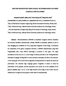
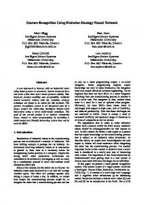
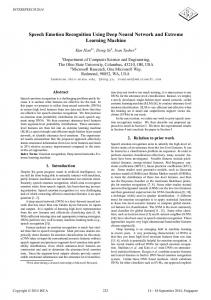
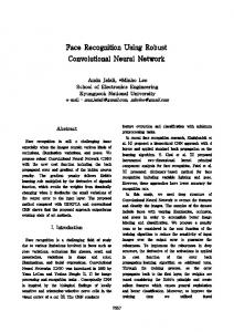
make it has the ability to store past participations and use this information from what has happened when it response to human [32, 33]. 1.2 DATA SET The data set used in this studies dubbed Corpus of Social Touch CoST, [34]. It comprises from 14 different touch gesture selected depending on, Yohanan‘s touch dictionary depending on the studies concern by touch interaction between humans and other humans and animals [28], the gestures set is shown in Table 1.1. This list of gestures is elected because it is similar to interaction of human with artificial arm . The data collected via 31 participants, where each one give paper contain some information about the procedure of data collection, and asked them to use their right hand to interact with mannequin arm, while their left hand is use to press the keyboard . The participants were asked to perform 14 gestures on a 8 × 8 array of pressure sensor grid wrapped around a mannequin arm (see Figure 1.1).The participants must press backspace key when s/he want to retry the current gesture, while they could press the space bar to perform next gesture. Figure 1.2 , shows the 14 gesture instances of each class for evaluation the summed pressure (y-axis) through time(x-axis) [35].

Figure ‎1.1: Set-up used in collecting the CoST . The black fabric around the mannequin arm measure the pressure.[34].

Each touch gesture can be performed in three levels of variations: gentle, normal, and rough. In addition the participants asked to repeat each gesture 6 times. Therefore each subject implement 252 gesture instance. For all participants, total recorded data 7812, but some data is lost after data preprocessing, the remaining data samples are 7805 as shown in Table 1.2, [34]. Before 3

participant began to perform gestures, each of them see a video that contain example for a person who perform all 14 gestures in three variations (i.e. gentle, normal and rough). These gestures were performed on the mannequin arm depending on the demonstration of each gesture that shown in Table 1.1,[34]. Therefore during the actual data collection, each participant shown the name of the gesture not the gesture definition, where the instruction display on a PC monitor for them. The pressure sensors can't sense the movement of the mannequin arm, so the gestures utilize movement of the arm itself for example, push, lift, and swing were neglected. The instruction of gesture was pseudo-randomized, so arranged there in three blocks. Table ‎1.1: Gesture definition adapted from [28]

Gesture label

Gesture Definition

Grab

Grasp or seize the arm suddenly and roughly.

Hit

Deliver a forcible blow to the arm with either a closed fist or the side or back of your hand.

Massage

Rub or knead the arm with your hands.

Pat

Gently and quickly touch the arm with the flat of your hand.

Pinch

Tightly and sharply grip the arm between your fingers and thumb.

Poke

Jab or prod the arm with your finger.

Press

Exert a steady force on the arm with your flattened fingers or hand.

Rub

Move your hand repeatedly back and forth on the arm with firm pressure.

Scratch

Rub the arm with your fingernails.

Slap

Quickly and sharply strike the arm with your open hand.

Squeeze

Firmly press the arm between your fingers or both hands.

Stroke

Move your hand with gentle pressure over arm, often repeatedly.

Tap Tickle

Strike the arm with a quick light blow or blows using one or more fingers. Touch the arm with light finger movements.

4

Figure ‎1.2: Gesture instance of each class (x-axis) for time and (y-axis) for summed pressure.

5

Table ‎1.2: Total CoST data set after loss some data [34] Variation Recorded Data

Gentle

Normal

Rough

Total

2604

2604

2604

7812

1 : massage Lost Data

1 : pat 1 : stroke

Active Data

2601

1 : tickle

1 : rub

1 : squeeze

1 : stroke

2602

2602

7

7805

Each instruction was given two times per block but the same instruction was not given twice in consecutive order. A single fixed list of instructions was constructed using these criteria. This list and the reversed order of the list were used as instructions in a counter balanced design [36, 37].When the participant complete recording the required gesture, s/he had press a key to see next instruction. After complete all experiment, the keystrokes were used to activate segmentation process. Each participant take almost 40 minutes to complete entire procedure. When block finished, the participant take break and asked to repeat instructions who faced some problems that prevent him from performing it. The participants must give their own description for gestures and the way to do this gestures [38]. 1.3 EXPERIMENTS SETUP The forearm of the mannequin arm (left hand) is full covered by array of sensors, and put on the shoulder (see Figure 1.1). The arm represents the human body part that is used to transfer emotions via touch. In addition the arm has ability to touch other body [4]. To record touch gestures an 8 × 8 pressure sensor grid (PW088/HIGHDYN from plug and wear) is connected to Teensy 3.0 USB microcontroller board via (PJRC), the size of sensor is 160 ×160 mm has 4 mm thickness and 20 mm for spatial resolution [34, 36, 37]. The sensor has the ability to sense the pressure from 1.8×10-³ to > 0.1 MPa at temperature of 25 c. After analog to digital ( A/D ) conversion, the sensor data is sampled at 135 Hz (frame per second). Therefore the duration of 6

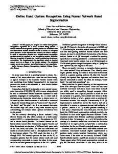
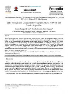
each gesture ranged from 75 milliseconds to 9.6 seconds [39]. 10 bits used , to transfer the pressure value of the 64 channels to integer number range from (0 to 1023). The textile used to manufacture the sensor which is comprised from five layers. The two outer layers manufactured from felt and used to protect the lower layers. Each one from covered layers including eight strips of conductive fabric isolated via non-conductive strips. These two conductive layers separates by sheet of piezoresistive material as middle layer. The conductive layers put in orthogonal form so it forms an 8 ×8 matrix. One of the conductive layers is attached to the power supply while the other is attached to the A/D converter of the Teensy board .Therefore the sensor satisfy the requirements set [40]. The instruction of each gesture that participant asked to perform it displayed to them by PC monitor m. During the data collection, the video recording as verification of the sensor data and the instruction given (see Figure 1.3). The data collect from this experiments include pressure value as intensity, per channel as location at 135 fps as temporal resolution [41]. The attributes of data set collected shown in Table 1.3.

Figure ‎1.3: Participant perform touch on the mannequin arm [36]

1.4 PARTICIPANTS To record the CoST data set, 32 people recruit to implement this task. One volunteer, could not completed the data recording, because of technical problems. Therefore the remaining participants was 31, consists of (24 males and 7 females). Their ages ranging from 21 to 62 years (M = 34, SD = 12) and 2 of them were left-handed. Also they are belonging to different nationalities such as; Dutch, Ecuadorean, Egyptian, German, and Italian. All of them are studied or worked at the University of Twente in the Netherlands.

7

Table ‎1.3: CoST data set characteristic [42] Attribute

Description

Number of touch gestures

14

Size of sensor grid

8×8

Sensor sample rate

135 Hz

Sensor range

0 - 1023

Gesture time

Variable

Gesture Interface

Mannequin arm

Gesture status

Gentle and normal

Number of participants

31 subjects

Train / test

21 / 10 subjects

Total number of touch gestures

7805 gestures

1.5 DEEP NEURAL NETWORK To be able to handle this huge amount of data, it is necessary to use one of the most powerful tools which has become very popular in the literature. Deep learning is an artificial neural network with interest of having deeper hidden layers. It recently surpassing the performance of classical methods in different fields especially pattern recognition [42]. The principle aim of Deep learning method is the learning feature hierarchies. The feature set that output from layer (L-1) is used as an input to the next layer (L) in the network. We can install the deep neural network by connecting non-linear nodes that take the raw input data and transfer it to higher level which was more abstract level. To transfer data from one layer to the next layer, the result of summation of previous layer should pass through non-linear function. The rectifier linear unit (ReLU), rectifier f(z) = max(z, 0), is the most popular non-linear function used with DNN [43]. Our candidate deep neural network is a Convolutional Neural Network (CNN).

8

1.6 CONVOLUTIONAL NEURAL NETWORK The most impressive forms of deep neural network and has excellent performance in many computer vision and machine learning problems. The Convolutional Neural Network (CNN) which can have multiple layers including convolutional layers, non-linearity layers, pooling layers, and fully-connected layers [44]. The primary application of the CNNs includes pattern classification and difficult image recognition. This makes encoding of images in multiple features, semantic segmentation, object detection in images, etc. possible using the high correlation between pixels within images [45, 46]. The input data to CNN usually a fixed size image, instead of handcraft features. The input image is convolved with different kernels to generate features map for the next layer. Therefore the learning method are very difficult in contrast to other machine learning methods such as multilayer perceptron [47].

The CNN

requires long time for training and testing the input image, because it repeatedly applies the deep convolutional network on the thousands of warped regions per image [48].The essential difference between CNN and traditional Artificial Neural Network (ANN) is that; the neurons in the CNN layer are organized into three dimensions. The input to CNN, is two dimensions is an image with a height and width, and the depth. The depth does not refer to the number of layers as in the standard ANN, but it refers to the number of features map in the CNN. Each neurons in the layer is connected to a small region of the previous layer [45].The CNN comprises from following layers. 1.6.1

Convolutional Layer

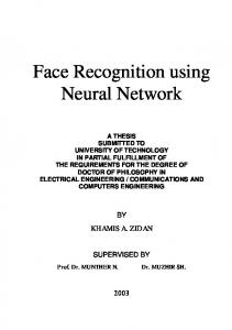
The convolutional layer will identify the number and the size of receptive filed of neurons in the layer (L) that is connected to a single neuron in the next layer using a scalar product between their weights and the region connected to the input volume. In convolutional layer, given the input, a weight matrix passes all over the input and the recorded weighted summation is placed as a single element of the sub sequent layer [45, 49]. As can be seen in Figure 1.4, the filter matrix (at the middle) are multiplied by the focus area (at the left matrix) which is shown by the green area and red color represents its center. It should be noted that this operation is not matrix multiplication operation, So, called element by element multiplication operation. The result of the multiplication operation will be stored at the corresponding place of the center of the focus in 9

the next layer. Then we can slide the focus area and fill the other elements of the convolution result (the right matrix). Moreover, in one layer, we can have multiple filter matrices (see Figure 1.5) to get parallel outputs corresponding to each filter in the next layer. Three hyper-parameters include (filter size , stride, and zero padding ) affects the performance of convolutional layer. By using different values for this hyper-parameters the convolutional layer will be able to decrease the complexity of the network [45].

Figure ‎1.4: Convolution Operation [51].

Figure ‎1.5: The multiple filters lead to multiple convolutional output [51]

1.6.2 Non-Linearity layer The non-linearity can be used to adjust or cut-off the generated output. There are many nonlinear functions that can be used in the convolutional neural network. However, Rectified Linear Unit (ReLU) is one of the most common nonlinearity functions applied in image processing applications (see Figure 1.6) . The aim goal of using the ReLU, it apply element wise activation function to the feature map from previous layer [45, 47, 50]. In addition the ReLU function transfer all value of features map to positive or zero [44]. The ReLU can be represented as shown in Eq.(1-1). ReLU(x)=[0 if x=0]

10

(1.1)

Figure ‎1.6: ReLU function [53]

1.6.3 Pooling Layer Pooling layer, roughly, reduces the dimensions of the input data and minimizes the number of parameters in the features map [45]. The simplest way to implement the pooling layer is by selecting the maximum of each region and then write it in the corresponding place of the next layer. Figure 1.7, shows a 2×2 pooling filter with a stride 2. Using this pooling filter reduces the input size to 25% of its original size. Also, averaging represents an another pooling method . However, taking the maximum is the most popular and promising method in the literature [48, 49, 51]. The maximum pooling method is non-invertible, so the original values before pooling operation cannot be restored . But if the locations of the maximum values of each moving in a set of switch variables are recoded, approximate original values can be generated [44].

Figure ‎1.7: Pooling decrease the dimension by mapping a region into a single element [48]

11

1.6.4 Fully-Connected Layer The fully-connected layer represents the last layers in any convolutional neural network. Each node in the layer (L) is connected directly to each node in layers (L-1) and (L+1). There is not any connection between nodes in the same layer in contrast with the traditional ANN [52, 53]. Therefore, this layer takes long training and testing time. At the same network more than one fully-connected layer can be used, as shown in Figure 1.8.

Figure ‎1.8: Fully-connected layer [56]

1.7 SUPPORT VECTOR MACHINE Support Vector Machine (SVM's) is the popular machine learning method and it is considered as one of the powerful and widespread algorithm used in classification algorithms. The SVM satisfy high classification ratio, and it has the ability to be applied on a multidimensional data, such as gene expression. In addition the SVM can deal with modeling diverse sources data [54, 55]. The essential factor that makes SVM perfect algorithm for multiple applications is it stability to find hyper plane which split the d-dimensional data into two classes . Furthermore, SVM's can be used to solve regression problem, where the output of the system become numerical values 12

instead of "yes/no" classification[56]. In machine learning algorithms, data split to training set and testing set. The target value (class labels) and other features are included in the training data, while data set contains the goal where the SVM try to produce a model that predicts the target values [57]. SVM is considered as one of the kernel methods algorithms. In such method a kernel function instead of the dot-product in some multi-dimensional feature spacer used. The kernel method has two benefits: has the ability to classify data with not clear dimensional vector space representation and it can be used as a linear classifiers to generate nonlinear decision boundaries[55]

13

2. RELATED WORK 2.1 INTRODUCTION Social touch gesture recognition is considered as an interesting topic for researchers in the last years. That is due to that the interaction between Human and machine has a lot of applications in human life. An important part of this researches working on designing and preparing the artificial skin equipped with arrays of sensors

that cover robot body. Another group of

researchers are interested to develop the robot and improve its ability to recognize and interpret the human gesture in a correct form. The robot designers are usually try to create robots that are important the daily life of people. Therefore the haptic creature looks like pets or Cartoon characters such as PARO, Huggable, PROBO and AIBO. So that children and people with chronic diseases can interact with this robots easily. In another aspects, various methods and algorithms try to classify and recognize the social touch in high accuracy, so haptic creatures can positive response to interaction human [58]. This chapter introduces a survey about the previous studies. The previous studies will be introduced in four main sections as follows:. 2.2 GENERAL REVIEW ABOUT SOCIAL GESTURE Lederman & Klatzky 1987 [59], To establish a relationship between required knowledge for objects with movements of the human hand. (Lederman & Klatzky) implemented two experiments by using the haptic object exploration. The first experiment depend on a match-tosample task. In which directed match between the subject with the particular dimension. The object exploration use the ―exploratory procedures,‖ to classify the hand movement . Each procedure has its properties that used by matching process. The second experiment, identified the reasons for special links that connect exploratory procedures with knowledge goals. During hand movement, the procedures are considered in terms of their necessity, sufficiency, and optimality of performance for each task. The results obtained explained that through free exploration. The procedure is generally used to extract the information about an object property. Because it is optimal or even necessary for this tasks. Reed at el. 1996 [60], They have tried to recognize the hand gesture in real-time using Hidden Markov Model (HMM) algorithm. The gesture recognition based on global features that 14

extracted from image sequences of hand motion image database. The database contains 336 images for dynamic hand gesture such as (hand wave, spin, pointing, and hand moving). These gestures are performed by 14 participants, each one performs 24 distinct gesture. The dataset is split to 312 samples for training and 24 samples for testing. The dynamic features extraction reduced the amount of data by 0.3 of the original data information. The system satisfied 92.2% gesture recognition accuracy. Naya at el. 1999 [20], Measured the human emotions depending on physical interface between human and pet like the robot. The interface made from gridded pressure -sensitive conductive ink sheets. Gridded sheets were made thin and flexible to cover the robot body. The robot interacts with the user via touch. The features which extracted for the data touch classification are absolute value, spatial distribution, and temporal differences in measured pressure patterns . The study has depended on five social touches that performed by 11 subjects and they are consisted of (slap, pat, scratch, stroke, and tickle). The recognition ratio for these five touches was 87.3% by using the k-Nearest Neighbor (kNN) algorithm. Cañamero & Fredslund, 2001 [21], Explained the response of "humanoid" LEGO robot for physical tactile. They have used stimulation rather than through other sensory modalities that do not require physical contact such as vision. They have displayed different emotions expressions as a result of social interaction between human and robot. The facial response of robot depends on the minimum set of features that needs to show the robot emotions and make it recognizable. The face emotions set that use in this work contains: anger, disgust, fear, happiness, sadness, and surprise. The experimental results show that the emotions of anger, happiness, and sadness are recognized easily. While the fear was mostly interpreted as anxiety, sadness, or surprise. The accuracy of results depend on the picture of human faces and the mental state. W. Stiehl & Breazeal, 2005 [13], The new type of robotic companion depends on touch interaction called (Huggable). Only the hand or gripper of the robot is covered by tactile sensor. The remainder surface remains not sensed. The neural network method was used for touch classification. Seven touches are used as the features such as (electric field, temperature, and force). Features extracted from a dataset which comprises from 200 samples. The neural network contains three layers. The Hidden layer has 100 nodes and the output layer with 16 nodes (9 for

15

the neural network class classifier, and 6 for the neural network response classifier).

The

effective touches are: tactile, poke, scratch, pet, pat, rub, squeeze and contact. W. D. Stiehl et al. 2005 [14], Explained the design and primary results of the touch classification for the Huggable robot which is covered by sensitive skin for its whole body. This robot was equipped by inertial measurement and embedded PC with wireless communication system. The PC use for Some processing that used for multi-modal interaction. The artificial skin is very important in the design and it must be soft with light touch. Three types of sensors was used with this robot. The first one is the electric field sensor to discriminate between a contact by human or by other objects. The second one, is the Quantum Tunneling Composites (QTC) sensor which is used to determine the direction of motion or for the size of contact. The third one is the temperature sensor which required a time constant less than QTC and electric field sensors. Colgan et al. 2006 [61], Using video clip to study the reaction of 9–12-month-old infants with autism to different gestures. The study introduces the interaction of child who is suffering from autism with the number and type of social gestures that develop nonverbal communication skill of children. Three types of touch functions were used in this study; joint attention, behavior regulation, and social interaction. These touch functions contain diversity type of gestures. The joint attention gestures refer to this attention body or case. The behavior regulation gestures refer to gestures that had ability to control the behavior of another gesture. Social interaction gestures refer to gesture that use to social interaction with other human. Haans & IJsselsteijn, 2006 [62], introduced a survey on the studies and the area implementation of mediated or remote emotion and felling transfer between distance people. They explained some issues related to mediated social touch. These issues include perceptual mechanisms, enabling technologies, theoretical underpinnings, and the methods or algorithms used to solve the problem of artificial skin. Bailenson et al. 2007 [7], Attempted to determine the emotions that transmitted by virtual interpersonal touch (VIT). They used feedback haptic device. People try to touch one another to find a framework that used to classify and understand facial emotions. Three experiments have been performed. In the first experiment the subjects asked to perform seven emotions (anger, disgust, fear, interest, joy, sadness and surprise). Depending on Two-Degree-Of-Freedom 16

(2DOF) force-feed back joystick. Tests different characteristic of the forces and subjective rating of difficulty of expressing of those emotions. In the second experiment another group of subjects try to determine the emotions performed by the first experiment group. Finally, in the third experiment pairs of subjects try to transfer and understand the seven emotions via physical handshakes. The result state that the subjects using virtual interpersonal touch (VIT) can communicate between them more easily than subjects who are using handshakes. Fang et al. 2007 [63], Proposed new method depending on hand gesture recognition for interaction between human and computer at real time. The hand was represented in multiple gestures by using elastic graphs with local jets of Gabor filter that use for features extraction. Users perform hand gesture used to recognize the gestures. The proposed method pass in three step. Firstly, hand image segment to color and motion cues generated by detection and tracking. Secondly, features are extracted by scale space. The last step is the hand gesture recognition. The recognition ratio was effected by camera movement in virtue of stable hand tracking. Boosted classifier tree was used to recognize the following six gestures: LEFT, RIGHT,UP, DOWN, OPEN and CLOSE. The number of frames that recorded in the experiment are 2596 frames. The frames that recognized correctly were 2436 and 93.8% correct classification ratio was achieved. Jia et al. 2007 [64], Described the design and implementation of intelligent wheelchairs (IWs). The motion of this wheelchair was controlled via a recognition of head gestures based on human and robot interaction (HRI). To satisfy the correct face detection at real time. The designer used hybrid method which contained Camshaft object tracking with face detection algorithm. The essential achievement of the intelligent wheelchairs involved autonomous navigation capability for good safety, such as Flexibility, mobility, obstacle avoidance, etc. In addition

to this

capabilities the interface between users and wheelchairs was provided with the traditional control tools (joystick, keyboard, mouse and touchscreen), voice-based control (audio), vision-based control (cameras) and other sensor-based control (infrared sensors, sonar sensors, pressure sensors, etc.). Wada & Shibata, 2007 [65], Designed a robot which is called Paro for house companion. Paro helps elderly people who are staying at their houses in daily life to support them to have their food and bathing. To study the nature of interaction between human and Paro. Two Paros were used in a public area more than 9 hours for a period of month. At the same time identify the 17

sociopsychological and physiological effects on the human resident at home every day. Through the experiment each subject was interviewed. A video cameras in the public area were used to record the activities of residents through the daytime for 8:30 to 10:00 hours. The urinary test explained that the stress and reaction of subject after interaction with Paro was improved. Breazeal, 2009 [66], Determined four important points that give the robot the ability to learn from environment by interaction with humans. The researchers tried to improve the expressive autonomous robots that be able to respond to people in a desired manner. make the robots learn new skills from people. Improved the robot to increase its ability and avoiding the effect of noise and the accuracy is more than traditional machine learning algorithms. Hertenstein et al. 2009 [4], Their study depended on the whole body to transfer different emotions between unacquainted partners. The partners put in rooms and each one can't see other. They are separated by barrier but they can communicate via hole in the barrier. Evaluate the accuracy of touches decoded by persons who receive a touch by their forearm without seeing tactile stimulation. They must determine the type of touch that she/he thought the encoder was sent. The emotions include anger, fear, disgust, love, gratitude, sympathy, happiness, sadness, surprise, embarrassment, envy, and pride. The classification accuracy for the first six emotions was better than the last six emotions. The data set of touch was performed by 248 subjects (124 unacquainted dyads). The age of participants was between 18 to 36 years (M = 19.93 and SD = 1.92 ). Each dyad are randomly divided into encoder and decoder. The gender of each pair (encoder-decoder) is divided to distinct four dyad as follows female-female (n = 44), female-male (n = 24), male-male (n

= 25), and male-female (n = 31). The correct

classification accuracy of decoded emotions was ranged from 48 % to 83 %. Knight et al., 2009 [15], Introduced a recognition system for social touch gesture at the real time. In addition, they have identified the requirement of hardware and software that used to build the robot. Full body of the robot (teddy-bear body ) was covered by sensors. Sensors have the ability to recognize both local touches like a poke or full body touches like a hug. The algorithms that used in the study depend on a real human interaction with the bear robot. The system was designed to detect three types of touches such as social touch, local touch, and sensor-level touch and eight distinct touches that include pet, poke, tickle, pat, hold, tap, shake and rub.

18

Kotranza et al. 2009 [11], Introduced the bidirectional touch interaction between human and virtual humans (VHS) as nonverbal communication. The bidirectional communication between two humans are very important. The body of virtual human was covered by haptic and the sensors were used for touch interaction with human. The (VH) are used for medical applications (doctor-patient interaction). Doctors try to touch patients to get on some information and to empathy, to comfort, achieve compliance, improve patient verbalization and attitudes. Yohanan et al., 2009 [12], Explored the essential property of affective touch in social interaction between human and robot in natural environment using Haptic Creature. They explained how the user's sensed an effect depending on both configuration and autonomous for companionship and therapy application. This haptic creature were used to determine the social touch that introduced by the human to express some emotions. In the same time the creature were used to identify the same issues to extract form factor, surface textures and movements, and how the robots can recognize them and how the human can express this emotion. To create online evolution for effective touch from physical sensors Both fuzzy logic and Hidden Markov Model estimation were used. This evolution were used to update the existed model of the user's emotional state. Chang et al. 2010 [3], Satisfied 77% classification accuracy for four distinct touches that contains stroke, slap, poke, and pat gestures. They depended on the first-generation of gesture recognition engine (GRE). Chang et al., also, studied the components of a physically interactive system (Haptic Creature) and analyzes its results. The obtained classification ratio using the error patterns suggested the sensor deficiency. The interaction between human and haptic creature across touch via a force-sensing resistor network, and communicates its internal state via purring, stiffening its ears and modulating its breathing and pulse. They used animal platform to prevent the confounding factors in human-human social touching such as gender. Dahiya et al. 2010 [30], Showed different techniques and method that used to build the touch sensors. The sensors were used to cover all or part of the robot body . The main issues of their study include the physiology, coding transferring tactile data and perceptual importance of the ―sense of touch‖. Kim et al. 2010 [24], Study were based on Temporal Decision Tree(TDT) algorithm and real interaction of robot with dynamic movement. Kim et al., used this method to classify the touch 19

through human and robot interaction. Their proposed algorithm were used to recognize four distinct touch gestures which consists of (hit, pat, push and rub). The gestures were performed via 12 participants (11 male and 1 female). The age range was from 24 to 38. The features that used to classify gestures were extracted from touch nature such as the time duration of the touch, the touch area of tactile and the movement of touch. They achieved 83% correct classification ratio of touch recognition. Tawil et al. 2011 [19], Covered the robot by flexible and stretchable artificial sensitive skin composed of electrical impedance tomography (EIT). This touch sensor was used to collect six different touch gestures that includes (tap, pat, push, stroke, scratch and slap). Performed via 35 participants. The features that used in gesture recognition consist of Maximum intensity value, Minimum intensity value, Spatial resolution at 50% of maximum intensity, Mean of intensities within the area of contact, Touch duration, Rate of intensity change and Displacement from initial to final location. The classification method that used for gesture recognition was ―LogitBoost‖ algorithm and the correct classification ratio was 80% of gestures. Yohanan & MacLean, 2011 [67], Explained the steps for designing Haptic Creatures emotion model to make robot interaction and communication with the human. If ignoring the human gender, and the correct state of response to human gesture. (Yohanan & MacLean), concluded that the robot recognizes the touch and responds in arousal state more effective than valence state. The dataset were performed by 32 participants (50% female). Each one from the participants was compensated CAD$ 10. The age start from 19 to 50 (M = 27.5, SD = 9.37). All of them were native English speakers and they did not deal with Haptic Creature before. Each one of the subjects selected one of sixteen emotions that includes afraid, angry, disgusted, happy, sad, and surprised, aroused, depressed, distressed, excited, miserable, neutral, pleased, relaxed, sleepy and none of these to evaluate the robot's emotional state. The correct classification rate for all subject was within the range from 17% to 52% (M = 30%, SD = 10%). Flagg et al. 2012 [16], Built a modern category of sensors depending on conductive fur. The conductive fur are affected by motion instead of conventional pressure sensors. It is used for interaction between human and robot. When the fur is touched by a human with hand movement, the electric current will be changed as fur's conductive threads connect and disconnect through touch interaction. By measuring this change in electric current the sensor capture motion. Seven 20

subjects were used to perform three gestures set which consists of stroke, scratch and light touch. The total number of data set made of 30 2-second samples each of stroke, scratch and light touch gestures, performed by one of the experiment. To choose the most important features for training the analytical methods and visual analysis of density curves were used. Then a logical regression model was used for training the data set, and the accuracy was measured on test set. The average classification ratio of gesture reorganization was equal to 82%. This result was obtained by using different machine learning schemes including a Bayesian network, multilayer perceptron and logistic regression using leave-one-out cross-validation. MacLean et al., 2012 [18], Introduced an overview about three issues. The first issue was about how human-robot interact via social touch. They determined the steps to design haptic creature that similar to pet robot, such as cat or dog that can be installed at a personal laboratory. In addition to study the response and emotions of this robot to effective touch. The second issue, explained the application that depends on haptic creature such as emotionally potent display. And the ability to build artificial

touch sensor to cover robot body. This sensor used to

communicate between human and robot for anxiety reduction. Finally, they tried to create devices that ―just do what you want them to‖, when use touch such as channel for feedback for a noisy control signal. Silvera Tawil et al. 2012 [68], Covered the full size of mannequin arm by

flexible and

stretchable artificial skin. Depending on electrical impedance tomography (EIT) principle, location, duration and the intensity information of the touch can be extracted using this skin. They obtained gesture recognition ratio equal to 71% . The data set was included eight distinct touch such as (tap, pat, push, stroke, scratch, slap, pull, and squeeze). Fourteen subjects were used to perform them. Individual and multiple subjects performed touch on an arm covered by sensitive artificial skin. The 'LogitBoost‘ algorithm was used as a classification algorithm. While the features used by the algorithm were based on Pressure intensity Point localization two-point discrimination threshold, Area of contact and Temporal information. The background of gender and cultural of participants were, also, examined. However they don't have any effect on classification result. Yohanan & MacLean, 2012 [28], Employed Haptic Creature similar to animal such as (cat or dog) that can sit on the human lap. They used this haptic creature to study the methods that the 21

human can interact with robot via touch, and the emotions response of the robot. The body of the robot was covered by layers of sensors. The sensor make the robot senses a human touch and move to express some emotions as adjusting the stiffness of its ears modulating its breathing and presenting a vibrio tactile purr. They used different human's intents with effective touch that includes protective, comforting, restful, affectionate and playful. Dataset was performed by 30 participants, half of them were female with ages from 18 to 41 years (M = 24.33, SD = 6.47). The haptic creature response consists of sixteen distinct emotions (afraid, angry, disgusted, happy, sad, and surprised, aroused, depressed, distressed, excited, miserable, neutral, pleased, relaxed, sleepy and none of these ). Flagg & MacLean, 2013 [1], Suggested new type of fur with an array of sensors used for humanrobot interaction via touch. The fur sensors

were equipped by

a piezoresistive fabric

location/pressure sensor. The sensors were used to cover curved creature. These fur sensors were used to gather data depending on two sensors. They, also, used to test nine different effective touch gestures performed by sixteen subjects (9 females). The touch gestures include stroke, scratch, tickle, squeeze, pat, rub, pull, contact without movement and no touch . The features that used for classification contain maximum, minimum, mean, median, area under the curve, variance and total variation. Machine learning algorithms were used for gesture recognition which satisfy correct classification ratio of 94% for trained

individuals. 86% correct

classification ratio as an average for all participant were achieved. Also, they obtained 79% correct classification ratio to recognize who is subject that touch the robot. Huisman et al. 2013 [9], enabled two-person who are transferring touch and felling between them in two places. The study used Tactile Sleeve for Social Touch (TaSST). The touch sensor of sleeve was equipped with grid of 4x3 sensor compartments filled with conductive motor. Three categories of prerecorded touch (simple, protracted and dynamic ) for six types of touch gestures were used in the study. The touch gestures include poke, hit, press, squeeze, rub and stroke. The touch gestures were performed by ten subjects (8 male, 2 female), with different ages (M = 28.3 ,SD = 2.9). Altun & MacLean, 2015 [25], Used furry robot pet (Haptic Creature). They collected nine different emotions which includes distressed, aroused, excited, miserable, neutral, pleased, depressed, sleepy and relaxed. These emotions were performed by 31 participants. The 22

participants asked to imagine the emotions located in a 2-D arousal-valence effect space. The features that was used to classify emotions consist of the time series‘ mean, median, variance, minimum, maximum and total variation. The Series Fourier transform and its peak and the corresponding frequency were added to features extracted. The Random Forests (RF) algorithm was selected to classify emotion depending on the features. The results of classification accuracy was 36% (all participants combined) and 48% (average of participants classified individually). Jeong et al., 2015 [69], Designed Huggable robot that has the ability to interact and emotions responds to children who are suffering from some chronicle diseases. These children need full time special care. In the same time this huggable robot can be used with many young patients who are nervous, intimidated and are socio-emotionally vulnerable at hospitals. The robot was covered by sensitive fur that make it friendly to users. It's computational power and array of sensors depending on the smartphone device. When a user touch the robot, the fur sensor deal with touch information in a signification manner. Four children were used to test huggable two of them were healthy and another two children are ill. All children spend happy time with robot. However, ill children were more enjoyed with robot. Ortega et al. 2015 [2], Suggested efficient method to solve gesture recognition rely on features that elicited from the dataset only. The finite state machine was used without the past learning samples. This method was easy to perform. Uriel Martinez-Hernandez et al., 2016 [32], Build an integrated probabilistic framework for perception, learning and memory in robotics. The essential part of this framework memory is Computational Synthetic Autobiographical. The Gaussian Processes used as a basis and mimics the functionalities of human memory. The memory type, that used with principled Bayesian probabilistic framework, has the ability to receive and process data from a lot of sources at different environment. The robot framework is called iCub humanoid robotic. It can detect and determine human face, touch gesture recognition when interact with human and the movement of arm based action recognition. Therefore, the robot has the ability to interact and learn from human. The correct classification rate for face detection was equal to 99.33%, 98.4% for arm movement, and 95% for touch gesture recognition.

23

U. Martinez-Hernandez & Prescott, 2016 [29], investigated how to control robot emotion that generates a response to a sensor touch and to recognize the distinct type of touch gesture . Bayesian with sequential analysis method was used with ten tactile datasets . This dataset was collected from the touches that performed on the sensor array that cover iCub humanoid robot. The study used five datasets for training and five data set for testing. The emotions of robot were represented by facial response. The result obtained from this method was used to control robotic emotions when human interact with the robot. The robotic emotions comprised happiness, shyness, disgust and anger. The proposed method satisfy average classification ratio of 89.5% when individual duration and pressure features were used. Cabibihan & Chauhan, 2017 [5], Illustrated the methods that used to send an effective touch from one person to another via the internet network using tele-touch tool. Instruction that sent by internet network to a haptic device at the subjects' forearm consists of vibration, warmth and tickle. In addition to a galvanic skin response (GSR) sensor and a heart rate (HR). The participants who are voluntarily do the test by email, comprises from three groups. Each group included ten healthy men, the ages range was from 18 to 30 years. The first group for control and it is called the no-touch (NT) group. The second group for human touch (HT), they will touch the subject through experiment. The last group evaluate the subjects of the tele-touch (TT) group in the time when the device start the test. At the end of the experiment, the result explain not important difference between HR of the subject with the tele-touch device from subject who touched via loved one. The result of GSR explained that all three touch groups were different from each one another. Jung et al. 2017 [6], Studied the effect of animal-like robots such as robotic seal Paro on the patients with dementia. They also introduced the interaction between patients and animal-like robot through touch. The animal-like robot has the ability to social interaction with patients by touch and speech which make the interaction more significant. The experiment conducted interviews with nine peoples suffer from dementia and divided to two group. The first group with 5 patients (expert group) who deal with Paro. The second group comprised from 4 patients they do not have any idea or used Paro before (the layman group). The experiment stated that the people with dementia developed well-being when interact with Paro by touch.

24

2.3 GESTURE RECOGNITION USED SVM Cooney et al. 2010 [70], Implemented a new tiny category of Sponge robot. The robot was covered by an array of sensors that has the ability to full-body touch gesture recognition, designed for interaction and play with the human. The dataset was collected by 21 volunteers. They performed 13 distinct gestures. Each gesture performed by at least two subjects. The touch gestures consists of Inspect, Up Down, Lay Down, Stand, Balance, Walk, Airplane Game, Dance, Upside-down, Rock Baby, Back and forth, Fight, and Hug. The study used 19 features for gesture classification that includes Mean values for accelerometer, Standard deviations for accelerometer, Overall ―trends for accelerometer , Medians for accelerometer, Minimums for accelerometer and Maximums for gyro. The correct classification ratio for gesture recognition was equal to 77%, using standard one-vs.-one RBF kernel Support Vector Machines (SVM). Ji et al. 2011 [71], Used KASPAR humanoid robot, child size, covered its hand, arms, feet, and torso by the touch sensor. The Eliminated the global location information and relied on a small data to represent huge data. The extracted features space of touch gesture samples was depended on the accuracy of a histogram of the tactile image. Therefore to get an information about spatial tactile patterns small amount of data are enough. The robot was used to recognize four distinct type of touches. The touches comprised from poking with the index fingertip, bar shape: contact with a full finger, gripping with three fingers "thumb, index, and middle fingers" , and gripping with the whole hand ).The SVM with the intersection kernel and Radial Basis Function (RBF) kernel algorithms were used to classify gestures. The 4-fold cross-validation is used to evaluate the accuracy of the algorithms. The touch recognition accuracy was 96% for (SVM) with the intersection kernel, and 93% for SVM with Radial Basis Function (RBF) kernel . Cooney et al. 2012 [72], Used a humanoid robot appearance to explain the ways that is used by people to transfer gesture between them. Gesture are transferred by touch or by vision, or both. They explained the sensor system that used to perform touches. The humanoid robot appearance was established by Typical Affectionate Behaviors (TAB). It includes typical touch gestures, their affectionate meanings, and their recognizability by a recognition system. The dataset was collected from 21 volunteers (12 males and 9 females). The mean and standard deviation of the age of subjects were 24.1 and 4.4, respectively. Data was split into two group; the first group included the subjects that touched the humanoid robot. While the second group used for 25

recognition method. The features extraction depended on the general modality specific requirement, touch location and the information were got from frequency or temperature. The accuracy of gesture recognition using the SVMs was 71.9%, 77.5% and 90.5% according to touch , vision and both gesture, respectively. While the accuracy results computed by using the k-Nearest Neighbor algorithm (k-NN) was 63.3%, 67.4% and 82.4, respectively. Nakajima et al., 2013 [73], Used balloon and put an array of barometric pressure sensor inside it. The surface of balloon was covered by soft interface of social touchable called "Emoballoon". The soft interface has the ability to sense the force of pressure when the human interacted with balloon. The dataset comprised of seven different touches that includes (hug, punch, kiss, rub, slap, grasp and press) performed by nine participants. The features used for touch gestures classification were extracted from different states of pressure on ―Emoballoon‖ . To evaluate the accuracy of touch gesture recognition the SVM with radial basis function (RBF) kernel was used and satisfy 83.5% correct classification ratio. 2.4 GESTURE RECOGNITION USED DEEP LEARNING ALGORITHMS Collobert & Weston, 2008 [74], Used Convolutional Neural Network (CNN), as a deep learning algorithm for Natural Language Processing (NLP) task. To classify input sentence to one of the speech parts. The speech comprised from named entity tags, chunks and parsing, semantic roles, semantically similar words and the likelihood. A Multitask learning (MTL) procedure was used for network training process. They used both the labeled tasks (supervised tasks) as multitask learning, and semi-supervised learning for the shared task. While an unlabeled text

as

(unsupervised model) used for learn the language model. (Collobert & Weston), used Wikipedia dataset that contains 631 Million words as a source for training and testing process. In MTL the task that trained at any layer was considered as a feature for another task. The proposed algorithm was applied on different tasks such as Semantic Role Labeling (SRL), Named Entity Recognition (NER), and Part-Of-Speech Tagging (POS). The MTL improved the results in the state-of-the-art performance. Saldien et al. 2008 [75], used of Deep Neural Network (DNN), for speech recognition in acoustic modeling. They described the ways that used to train the DNN. Two-step of training methods were used to perform DNN fitting . In the first step, fitting the stack of generative models. 26

Initialized the layers of feature detectors. This steps make the generative models are training without using any information for Hidden Markov Models (HMM). At the second step, all generative model in the stack used to initialize one layer of hidden units in a DNN and the whole network is then discriminatively fine-tuned to predict the target HMM states. To test the accuracy of these two steps of DNN training. The TIMIT was used as dataset for speech recognition in acoustic modeling. The result of recognition accuracy was very acceptable and outperformed other methods. Lee et al. 2009 [76], Applied the convolutional deep belief networks (CDBN) on the corpus of phonemically and lexically transcribed speech of American English speakers of different sexes and dialects. Each transcribed element has been delineated in time called (TIMIT). The algorithm used to classify an

unlabeled auditory data that includes speech and music. Audio classification was used for assessing the learned feature representations. When speech data were used, the learned features correspond to phones/phonemes, and outperforms other feature spectrogram and Mel-frequency cepstral coefficients (MFCC). The audio data that fed to CDBN must be converted from time domain to spectrograms. Then the principal component analysis (PCA) is used for spectrograms dimensional reduction. The result of this system satisfied high classification ratio for multiple audio recognition tasks. Krizhevsky et al. 2012 [77], Used a Big and deep convolutional neural network (CNN), which consist from 650,000 neurons and 60 million parameters. The CNN was distributed among five convolutional layers, followed by max pooling in some layers, with three fully-connected layers, followed by 1000-way softmax. The input to the network was 1.2 million high-resolution images (256 x 256 -pixels) used for network training 50,000 validation images, and 150,000 testing images. The input was a subset from ImageNet Large-Scale Visual Recognition Challenge (ILSVRC-2012). The images were divided into 1000 different groups. 1000 images for each group, thus the network required to long time to train 1.2 Million images. Therefore GPU implementation used to decrease the time that need for training. Dropout method was used to eliminate the overfitting problem at the fully-connect layers. The satisfied result of top-1 and top-5 error rate when applying the network on the test data were 37.5% and 17% ,respectively. Mohamed et al. 2012 [78], Proved that using the DNN includes a lot of features with huge number of parameters introduces very good result of speech recognition (acoustic modeling) . 27

These findings were obtained when the DNN is applied on the TIMIT dataset. A multilayer of generative model of window of spectral feature vectors were used to initial pre-training the network. The generative pre-training was firstly considered as features to get a good results of prediction for probability distribution over the states of monophonies Hidden Markov Models (HMM). The backpropagation method was chosen to implement the discriminative fine-tuning, that used to regulate features. The advantages of pre-training was to let the network use huge number of parameters to avoid overfitting problem. And to facilitate the development process of the DNN that comprises of multilayer of hidden nodes. The phone error rate by using DNN was equal to 20.78 %, this result is more accurate than the result obtained by the previous methods. Abdel-Hamid et al. 2013 [79], Computed and compared the results of CNN, using different aspects. They checked the architectures, which consists of full and limited weight sharing. They investigated the convolution for frequency and time axes, and the number of convolutional layers. Also the size of pooling layer become automatically learned depending on weighted softmax pooling layer. Test the effect of pre-training that can satisfied by using Restricted Boltzmann Machine (RBM) on the performance of the CNN. Two dataset were used , the TIMIT and Microsoft internal voice search (VS). While the features extraction were similar for both data set. The results of phone error ratio (PER) for system without pre-training was between 20.5% to 22.5% for different architectures and parameters. While the value of PER for system with pre-training was between 20.5% to 22.8%. Han et al. 2014 [80], Proposed new effective method for speech emotion recognition (acoustic modeling). They depended on the extracted important features from the raw data. They used these features as an input to the DNNs. The DNN was used to generate an emotion state probability distribution. The utterance-level features were built from segment-level probability distributions. The utterance-level features used as an input to extreme learning machine (ELM). The results explained that the proposed method achieved a 20% relative accuracy improvement compared to the state-of-the-art approaches. Karpathy et al., 2014 [81], Applied the CNN to classify the Sports-1M dataset. The dataset includes 1 million YouTube videos divided into 487 categories . The dataset was divided into 70% of the videos as training set, 10% as validation set and 20% as a testing set. They used histogram as a feature for classification and to capture the advantages of local spatiotemporal 28

information.. Using spatiotemporal for networks explain achieving 63.9%

performance rate

compared to 55.3% achieved by strong feature-based baselines. While when retraining the top layers of the UCF-101 using the proposed method the performance improved to

63.3 %

compared to only 43.9 % for the UCF-101 baseline model. Zhou et al. 2014 [82], Used Place data set which contain more than 7 million labeled images of scenes divided into 476 place categories. That is considered as scene-centric database. For scene recognition task, the CNN composed of 7 layers, and soft-max layer as an output layer. The CNN was used to learn deep features. The Place dataset is split into 2,448,873 images to training with 205 categories, and 100 images per category for validation. While test set consists of 200 images for each category. The performance of image recognition for Place database was evaluated using top-5 error rate on the testing set. The result of error rate was 18.9% . The CNN layer's responses determine the variation of internal representations of object-centric and scenecentric networks. Oquab et al. 2015 [83], Used the weakly supervised CNN. The network consists of 5 convolution layers and 4 fully-connected layers. They performed object classification, depending only on image-level labels, that have the ability to learn from cluttered scenes that includes more than one object. To evaluate the performance of CNN, two types of data set was used. The first one is Pascal Visual Object Classes VOC 2012 (20 object classes) which consists from 5000 images for training and 5000 images for validation. The second one was the data set was very large, Microsoft Common Objects in Context COCO (80 object classes). It included 80,000 images for training and 40,000 images for validation. The size of RGB image used in the study was 224 x 224 pixels. The result of object classification for VOC 2012 data set was equal to 82.3% and for location prediction was equal to 74.8%. While for Microsoft COCO dataset the classification rate was 62.8% and 42.9% for object classification and location prediction, respectively. Tamura et al., 2015 [84], Increased the efficiency of the performance for Audio-Visual Speech Recognition (AVSR) approach. They depended on three aspects. The First one, to improve the performance features for visual speech recognition by applying the Deep Belief Network Features (DBNF) method. The second one, to develop the performance of AVSR, they used the visual features and audio DBNFs. Finally, to avoid error of voice and audio recognition in silence period for lip-reading, the visual Voice Activity Detection (VAD) 29

was used. The

conventional Mel-Frequency Cepstral Coefficients (MFCCs) are used for features extraction. For training these features, an audio Gaussian Mixture Models- Hidden Markov Model (GMMHMM) were used. The results obtained from this methods was 73.66% lip-reading accuracy of recognition for speaker-independent open condition and 89.87% AVSR on environment affected by noise. Xiong et al. 2016 [85], Proposed new method to regularize, satisfy best generalization and decreases the overfitting problem. The method was called Structured De-correlation Constraint (SDC). Through the training process, the SDC encouraged the network to learn structured representation using grouping of hidden nodes. Then motivate this node in same group to build robust connections. At the same time stimulate the nodes in different groups to learn nonredundant representations via loss the cross-covariance between them. Different types of CNN architectures were used. The CNNs comprised from convolution, pooling, and fully-connected layers. The network Applied on three types of data set that includes, CIFAR-10 dataset which consists of 60,000 (32 x 32 pixels) RGB images, and 10 classes, 6000 images for each class, split to 50000 images for training and 10000 for testing. The accuracy of image recognition was equal to 6.22% . Second data set was the CIFAR-100 data set which consists of 100 classes, 600 images for each class, and split to 500 image for training and 100 image for testing. The accuracy of image recognition was equal to 9.63% . The third type was SVHN dataset, includes 73257 images, split to 531131 images for training , and 26032 images for testing. The accuracy of image recognition was equal to 95.5%. 2.5 GESTURE RECOGNITION APPLIED ON COST DATA SET Jung, 2014 [37], Used the Gaussian Bayesian classifiers, and SVM algorithms for gesture recognition. These two algorithms were applied to Corpus of Social Touch (CoST). The CoST includes 14 distinct touches (Grab, Hit, Massage, Pat, Pinch, Poke, Press, Rub, Scratch, Slap, Squeeze, Stroke, Tap, Tickle). Touches were recorded via pressure sensor. The CoST data set consists of 7805 touch gesture samples performed by 31 (24 males, 7 females) subjects. The age of the subjects was between 21 to 62 years (M = 34,SD = 12). Each subject performs 3 variations (normal, gentle and rough) for each touch and repeats each touch 6 times. The features set that used as an input to the recognition systems were consisted of 28 features (Mean pressure, 30

Maximum pressure, Pressure variability, Mean pressure per column (8 features), Mean pressure per row (8 features), Contact area(2 features), Peak count (2 features), Displacement (4 features), Duration ). The result of touch gesture recognition for Bayesian classifiers depending on these features was from 26% to 74% (M = 53%,SD = 11%). While for the SVM the gesture recognition rates was from 22% to 63% (M = 46%,SD = 9%). Jung et al. 2014 [34], Classified the gestures using Bayesian classifier and the SVM methods to create a baseline . The features set that used as an input to recognition systems consists of 28 features (Mean pressure, Maximum pressure, Pressure variability, Mean pressure per column (8 features), Mean pressure per row (8 features), Contact area(2 features), Peak count (2 features), Displacement (4 features), Duration. For the Bayesian method, the results range was from 24% to 75% (Mean = 54% and SD = 12%) . While for the SVM, the results range was from 32% to 75% (Mean 53% and SD = 11%). Van Wingerden et al. 2014 [86], Divided the CoST dataset into 35% training and 65% testing. The training data was used to select the best parameters for the NNs. Their NN architecture has one hidden layer containing 64 neurons. The essential features were selected based on the energy histogram and dynamic features include (Histogram-based features (8 features), Motion-based features (4features), Derivative-based features (3 features), Temporal features, Mean segmented temporal features), in addition to the basic features used in. The best performance they have achieved using all features was 64.6%. However, using the leave-one subject- out cross validation, they could only obtain 54% (SD=15.0%). Balli Altuglu & Altun, 2015 [87], Split CoST dataset as 65% for training and 35% for testing. The Random Forests (RF) algorithm was used as the tool for touch gesture recognition. They achieved a classification rate between 26% to 95%. The mean classification was 55.6% for 14 social touches depending on the sequential forward floating search. The features employed in the model included pressure data, an image feature, a Hurst exponent, Hjorth parameters, and autoregressive model coefficient features. These features was chosen by applying a sequential floating forward search (SFFS) algorithm. The total features became 42 features. Also test their method on a second dataset, Human-Animal Affective Robot Touch (HAART). The dataset

31

consists of 7 different touch gestures (no touch, constant, pat, rub, scratch, stroke, tickle ) and satisfies classification ratio between 60% to 70% based on 133 selected features.

Jung et al. 2015 [88], Summarized the challenge technique that face recognition algorithms and compared the results that obtained from these algorithms. They depended on the touch gestures that used with the 2015 ACM International Conference on Multimodal Interaction (ICMI). The study explained some important issues such as (1) Although the authors used different type of methods for touch gestures recognition, the confusion matrix was similar. (2) Different types of ways that used for features extraction consists of image processing, speech, and human action recognition provided valuable feature sets. The results of these distinct methods were different depending on the type of features used and the type of preprocessing.

Gaus et al., 2015 [41], Studied the ability to differentiate the social touch gestures category using two methods, Random Forest, and Boosting. The recognition methods were applied to two types of data set. The first one was the HAART. Which consisted of 7 distinct gestures performed by 7 participants. The HAART dataset split into 4 subjects for training and 3 subjects for testing. The second data set was called the Corpus of Social Touch (CoST). Which consisted of 14 distinct gestures performed by 31 participants. The CoST dataset split 21 subjects for training and 10 subjects for testing. The two datasets are available by the Social Touch Gesture Challenge 2015. To test the performance of the proposed methods five different set of high-level features were extracted. The extracted features Included Statistical distribution (SD) of pressure surface, Binary Motion History (BMH), Motion statistical distribution (MSD), Spatial Multi-scale Motion History Histogram (SMMHH) on touch dynamic, Local Binary Pattern on Three Orthogonal Place (LBPTOP) on touch dynamic. The result of touch gestures recognition were 67% correct classification ratio (CCR) for the HAART and 59% (CCR) for the CoST testing dataset.

Hughes et al. 2015 [39], Used Deep autoencoders as a DNN, and Hidden Markov Model (HMM). They classified the CoST and the HAART gesture sets. That used in Social Touch Gestures Challenge for ICMI 2015 to achieve high accuracy for gesture recognition. The gesturelevel features were used. Seven distinct features extracted form data set depending on, maximum 32

value of pressure through a touch, the area of pressure on the sensor, and how many gestures repeated at the touch. The CoST dataset was split into 21 subjects for training and 10 subjects for testing. The gesture recognition accuracy was 56% for Cost data set. While HAART dataset was split to 4 subjects for training and 3 subjects for testing, the gesture recognition accuracy was 71%.

Ta, Johal, Portaz, Castelli, & Vaufreydaz, 2015 [89], introduced an improved gesture recognition method and applied it on the CoST data set after applying it to HAART data set directly. They depended on three categories of features that includes 273 features divided as Global features, consist of 40 features, represent overall statistics of the gesture. Channel-based features consisted of 192 features, describe the spatial relationship between different channels. The sequence of average pressure features, consisted of 41 features, used the sequence of average pressure over all channels for each frame. The SVM and Random Forest (RF) methods used as a classifier for this two data set. A 3-fold Cross-validation was used to evaluate the performance of the proposed methods. The recognition accuracy for CoST dataset were 60.51% and 60.81% for SVM and RF, respectively. While for HAART data set the recognition accuracy were 68.52% and 70.91 for SVM and RF, respectively.

Jung et al. 2017 [36], Illustrated the step of dataset collection of the CoST in details. The CoST data set consists of 7805 sample of 14 distinct social touch gestures. The dataset was collected by 31 participants, each performed all gestures in three levels: gentle, normal and rough on a pressure sensor grid wrapped around a mannequin arm and repeating each gesture 6 times. 54 features were extracted from the dataset include Mean pressure, Maximum pressure, Pressure variability, Mean pressure per row, Mean pressure per column, Contact area per frame, Temporal peak count, Traveled distance, Duration of the gesture, Pressure distribution, Spatial peaks, Derivatives, Variance over channels, Direction of movement, Magnitude of movement, Periodicity. The data was split into training and testing set. Leave-one-subject out cross validation was used to evaluate the accuracy of gesture recognition. Four methods of machine learning were applied to the data set to compare their performance and results. The Bayesian classifier achieved 57% (SD = 11%) correct classification ratio (CCR). The Decision tree

33

algorithm introduced 48% (SD = 10%) CCR. SVM with RBF kernel 60% (SD = 11%) CCR and for the NN 59% (SD= 12%) CCR was achieved.

34

3. FUNDAMETAL OF CONVOLUTIONAL NEURAL NETWORK AND SUPPORT VECTOR MACHINE 3.1 INTRODUCTION In this chapter, we will explain theoretical fundamentals of algorithms that are used in this thesis. The first section illustrates the deep learning concept especially Convolutional Neural Network (CNN), the Second section introduces Support Vector Machine (SVM) algorithms and the last section explains dimensionality reduction technique and t-Distributed Stochastic Neighbor Embedding (t-SNE). 3.2 DEEP NEURAL NETWORK The term Deep Learning or Deep Neural Network refers to Artificial Neural Networks (ANN) with multilayers. Over the last few decades, it has been considered to be one of the most powerful tools and has become very popular in the literature as it is able to handle a huge amount of data[45]. The interest in having deeper hidden layers has recently begun to surpass classical methods performance in different fields; especially in pattern and image recognition [46, 90]. One of the most popular deep neural networks is the CNN. It takes this name from mathematical linear operation between matrices which is called convolution. CNN has multiple layers; including convolutional layer, non-linearity layer, pooling layer and fully-connected layer. The convolutional and fully-connected layers have parameters but pooling and non-linearity layers don't have parameters[91, 92]. The CNN has excellent performance in machine learning problems, especially the applications that deals with image data. Such as largest image classification dataset (Image Net), computer vision and in natural language processing (NLP), the results achieved by CNN are very interesting[81]. In this chapter, we will explain and define all the elements and important issues related to CNN, and how these elements work. In addition, we will also state the parameters that affect the efficiency of CNN. 3.2.1

Convolutional neural network

The CNN has had groundbreaking results over the past decade in various fields that related to pattern recognition; from image processing to voice recognition. The most beneficial aspect of 35

CNN's is reducing the number of parameters that required in Artificial Neural Network ANN [50, 51]. This achievement has prompted both researchers and developers to approach larger models in order to solve complex tasks, which was not possible with classic ANNs. The most important assumption about problems that are solved by CNN should not have features which are spatially dependent [46, 48, 49]. In other words, for example, in a face detection application, we do not need to pay attention to where the faces are located in the images. The only concern is to detect them regardless of their position in the given images. Another important aspect of CNN is to obtain abstract features when input propagates toward the deeper layers. For example, in image classification, the edge might be detected in the first layers, and then the simpler shapes in the second layers, and then the higher level features such as faces in the next layers as shown in Figure 3.1, [92-94]. We can describe the CNN layers by two types of terminology as shown in Figure 3.2. The first terminology called simple layer terminology (on the right hand side of the figure), where the convolutional net is viewed as a cascaded number of simple layer. Every layer after complete its data processing push its output results to the subsequent layer [95]. The second terminology is called complex layer terminology (on the left hand side). In such terminology, the convolutional net is viewed as a small number of relatively complex layers, each layer have many ―stages‖ [51]. To obtain a good grasp of CNN, we start with its basic elements. 3.2.1.1. Convolution Convolution is per-pixel operations, the same mathematical operation applied to all pixels in the image or frame. Therefore, the complexity and time required to perform convolution operations increase when the size of image or frame increase. A filter (sometimes called kernel) is a twodimension matrix of real numbers, or a smaller-sized matrix in comparison with the input dimensions of the image or frame. The filter coefficients varies from application to another [91]. To perform convolution, filter slides over image or frame from the upper right corner of the image and pass over every pixel till the lower left corner of the image. The image region that is under the filter called receptive field, which is the same size of the filter.

Convolution is

performed by multiplication operation between each number of the kernel and the corresponding value of image or frame and summation the result of multiplication. 36

Figure ‎3.1: Learned features from a CNN [95]

37

Figure ‎3.2: Components of a typical CNN Layers [97]

Then, the output is normalized by the summation of filter kernel. The result value becomes the new intensity of the pixel under the center of the kernel as shown in Figure 3.3, [96]. Figure 3.4 (a and b ) explains how the filter slide over input image or frame and inserting the result of convolution operation in the output feature map. From Figure 3.4, we can see that the size of output is smaller than input image size [91]. If we have RGB image (three channels), three filters for convolution operation should be used. Therefore the dimensions of this filters

38

was 3x3x3, each 3x3 filter is used for a single channel to produce one feature map in the output, as shown in Figure 3.5, [94].

Figure ‎3.3:The operation of convolution layer slides the filter over the given input [99].

To illustrate the operation of convolution , let us assume that the input of our neural network has the presented shape as in figure 3.6, It can be an image (e.g. color image of a CIFAR-10 dataset with a width and height of 32×32 pixels, and a depth of 3, which is the RGB channels) or a video (gray scale video whose height and width are the resolution, and the depth are the frames) or even the application in this thesis which has width and height of 8x8 sensor values and depth are associated with different time frames [47, 49]. So, why convolution ? Let us assume that the network receives raw pixels as input. Therefore, to connect the input layer to only one neuron (e.g. in the hidden layer in the Multi-Layer perceptron), as an example, there should be 32×32×3 weight connections for the CIFAR-10 dataset.

39

If we add one more neuron into the hidden layer, then we will need another 32×32×3 weight connection, which will become in total, 32×32×3×2 parameters. To make it clearer, more than 6000 weight parameters are used to connect the input to just only two nodes. It may be thought that two neurons might not be enough for any useful processing for an image classification application. To make it more efficient, we can connect the input image to the neurons in the next layer with exactly the same values for the height and width. It can be assumed this network is applied to the type of processing such as the edge of the image.

(a)

(b) Figure ‎3.4:(a & b) Sliding the filter over input image and put the result in output feature map [97]

40

Figure ‎3.5:Depth corresponding to the number of filters we have used for the convolution operation in the network [51].

Figure ‎3.6:Three-dimensional Input representation of CNN [100].

41

However, if we connect all nodes of input to all nodes of hidden layer the mentioned network needs 32×32×3 by 32×32 weight connections, which are (3,145,728), [44, 50, 97]. Therefore, looking for more efficient method, it emerged that instead of a full connection, it is a good idea to look for local regions in the image instead of the whole image. Figure 3.7, shows a regional connection for the next layer. In other words, the hidden neurons in the next layer only get inputs from the corresponding part of the previous layer. For example, it can only be connected to 5×5 neurons. Thus, if we want to have 32×32 neurons in the next layer, then we will have 5×5×3 by 32x32 connections which is 76,800 connections(compared to 3,145,728 for full connectivity [42, 45, 91, 94].

Figure ‎3.7: Convolution as the alternative for the fully connected network [100].

Although the size of connection drastically dropped, it still leaves so many parameters to solve. Another assumption for simplification is to keep the local connection weights fixed for the entire neurons of the next layer. This will connect the neighbor neurons in the next layer with exactly the same weight to the local region of the previous layer. Therefore, it again drops many extra parameters and reduces the number of weights to only 5×5×3=75 to connect 32×32×3 neurons to 32×32 in the next layer [92, 98, 99].

42

There are many benefits to these simple assumptions. Firstly, the number of connections decreases from around 3 million to only 75 connections in the presented example. Secondly, and a more interesting concept, is that fixing the weights for the local connections is similar to sliding a window of 5×5×3 in the input neurons and mapping the generated output to the corresponding place. It provides an opportunity to detect and recognize features regardless of their positions in the image. This is the reason why they are called convolutions [47, 50]. To show the astounding effect of the convolution matrix, Figure 3.8, depicts what will happen if we manually pick the connection weight in a 3×3 window. As we can see from Figure 3.8, the matrix can be set to detect edges in the image. These matrices are also called filters because they act like the classic filters in the image processing algorithms. However, in the CNN, these filters are initialized, followed by the training procedure shape filters, which are more suitable for the given task. To make this method more beneficial, it is possible to add more layers after the input layer. Each layer can be associated with different filters. Therefore, we can extract different features from the given image. Figure 3.9 (a and b), shows how they are connected to different layers. Each layer has its own filter and therefore extracts different features from the input. The neurons shown in Figure 3.9, use different filter, but look at the same part of the input image [91, 92, 94]. The performance of convolution operation is affected by some factors such as; size and number of filters, stride, and zero padding. In the next sections, we will explain the effect each factor on the convolution performance.

43

Figure ‎3.8: Effects of different convolution matrices [103].

44

(a)

(b) Figure ‎3.9: Multiple layers which each of them corresponds to different filter (a) looking at the same region in the given input image, (b) looking at the different regions in the given input image [51].

45

A. Size and number of filters The size and number of filters have directed effect on size and number of output features maps. The number of features maps always equal to the number of filters used in convolution operation. In addition the depth of filters used must equal to the number of input channels (e.g., if we have 96 features maps from first convolutional layer and we use 256 filters have size 5x5, therefore we must use 256 filters each one has size 5x5x96 ). While the size of filters used will be effective on size of output features maps. When filter size increase, the size of output feature map decrease, and vice versa.

B. Stride De facto, CNN has more options which provide a lot of opportunities to even decrease the parameters more and more, and at the same time reduces some of the side effects. One of these options is stride. We can define stride as the number of pixels by which we slide filter over input image or frame matrix. Therefore when we say stride equal 1, this means we move filter one pixel only over the input image, while when say stride equal 2, this means we jump filter two pixels at each move. In the above-mentioned example, it is simply assumed that the next layer's node has lots of overlaps with their neighbors by looking at the regions. We can manipulate the overlap by controlling the stride. Figure 3.10 (a and b), shows a given filter with size 3x3 and 5x5-pixelimage. If we move the filter one node every time, we can have a 3x3 output only. Note that the output of the matrices in have an overlap. However, if we move and set every stride 1, then the output will be 3x3. But simply, not only overlap, but also the size of the output will be reduced [47, 100]. Eq. (3-1), formalize this, given the image N×N dimension and the filter size of the F×F, the output size is O as shown in figure 3.11. (3.1)

Where N is the input size, F is the filter size, and S is the stride size. 46

(b) Figure ‎3.10: (a), 3x3 filter, (b), Stride 1, the filter window moves only one time for each connection [56].

Figure ‎3.11: The effect of stride on the output size [105].

47

C. Padding One of the drawbacks of the convolution step is the loss of information that might exist on the border of the image. Because they are not captured when the filter slides, they never have the chance to be seen. A very simple, yet efficient method to resolve the issue, is to use zeropadding. To control the output of convolution operation and at the same time to include the border pixels of input image or frame, zero padding is inserted to the border of the input matrix. In this case, we can slide the filter over all input matrix [94]. The other benefit of zero padding is to manage the output size. For example, in Figure 3.12, with N=7 and F=3 and stride 1, the output will be 5x5 (which shrinks the 7x7 input) [44, 97]. However, by adding two zero-padding, the output will be 7×7, which is exactly the same as the original input (The actual N now becomes 9, use the eq. (3-1). The modified formula including zero-padding is Eq. (3-2). (3.2) Where P is the number of layers of the zero-padding (e.g. P=1 in Figure 3.12), This padding idea helps us to prevent network output size from shrinking with depth. Therefore, it is possible to have any number of deep convolutional networks[101, 102].

Figure ‎3.12: Zero-padding operation [105]

48

D. Features of the CNN The weight sharing brings invariance translations to the model. It helps to filter the learned feature regardless of the spatial properties. To select best values for filter that used in convolution operation. We starting with random values for filters, they will learn to detect the edge (such as in figure 3.8) if it improves the performance. It is important to remember that if we need to know that something is spatially important for a given input, then it is an extremely bad idea to use shared weight. This concept can be extended to different dimensions also. For example, if it is sequential data, such as an audio signal, then it can employ a one-dimensional convolution can be used. If it is an image, two-dimensional convolution can be applied. And for videos or 3D images, a three-dimensional convolution can be used. This simple idea beat all the classical object recognition methods in computer vision as in the 2012 ImageNet challenge as shown in Figure 3.13, [50, 77]

Figure ‎3.13: Visualizing Convolutional deep neural network layers [80].

E. Convolutional Formula The convolution for one pixel in the next layer is calculated according to the Eq. (3-3)

49

∑∑

(3.3)

. Where

is the output to the next layer,

is the input image and

is the kernel or filter

matrix and is the convolution operation. Figure 3.14, shows how the convolution works. As it can be seen from Figure 3.14, the element by element product of the input and kernel is aggregated, and then represents the corresponding point in the next layer [44, 51, 93].

Figure ‎3.14: Details on Convolution layer [108]

3.2.1.2. Nonlinearity The next layer after the convolution is the non-linearity layer. The non-linearity can be used to adjust or cut-off the generated output. This layer is applied in order to saturate the output or to 50

limit the generated output. The non-linearity layer always is embedded within convolution layer [92, 96]. For many years, sigmoid and tanh were the most popular non-linearity functions. Figure 3.15, shows the common types of nonlinearity functions. However, recently, the Rectified Linear Unit (ReLU), as shown in Figure 3.16, has been used more often for the following reasons [46, 103]. 1. ReLU has simpler definitions in both function and gradient as shown the following two equations: (3.4) (3.5) 2. The saturated function such as sigmoid and tanh cause problems in the back propagation. As the neural network design become deeper, the gradient signal begins to vanish, which is called the "vanishing gradient". This happens since the gradient of those functions is very close to zero almost everywhere but the center. However, the ReLU has a constant gradient for the positive input. Although the function is not differentiable, it can be ignored in the actual implementation [14]. 3. The ReLU creates sparser representation, because the zero in the gradient leads to obtaining a complete zero. However, sigmoid and tanh produces non-zero results from the gradient, which might not be in favor for training [49, 93].

Figure ‎3.15: Common types of nonlinearity functions [94].

51

Figure ‎3.16: Rectified Linear Unit [94].

3.2.1.3. Pooling Layer There are two reasons to use pooling in CNN. Firstly, the output feature map of pooling is fixed size, which is required for the classification process. For example, if you have 256 filters and you apply max pooling to each, you will get a 256-dimensional output, regardless of the size of your filters. Secondly, the essential task of pooling is down-sampling in order to reduce the complexity for further layers. In image processing applications, it can be considered as similar as resolution reduction. Pooling does not affect the number of filters. Max-function is one of the most common types of pooling methods. It partitions the image into sub-region rectangles, and it only returns the maximum value of the each sub-region. One of the most common sizes used in maxpooling is 2×2. As shown in Figure 3.17 (a), when pooling is performed in the top-left 2×2 blocks (pink area), it moves 2 and focuses on the top-right part. This means that stride 2 is used in the pooling. Figure 3.17 (b) explains pooling operation for single feature map. To avoid downsampling, stride 1 can be used, but it is not common. It should be considered that down-sampling does not preserve the position of the information. Therefore, it should be applied only when the presence of information rather than spatial information is important [42, 48, 104]. Moreover, pooling can be used with non-equal filters and strides to improve the efficiency. For example, a 3x3 max-pooling with stride 2 keeps some overlaps between the areas. In addition for the above mention reasons, pooling layer controls the network over-fitting by eliminating the 52

number of parameters and the computation used in the network, and it scales the staple representation of input image. Therefore pooling motivates the network to be very invariant to the small change in the input image such as transformation, distortions, translation [105]. Further, there are other pooling methods such as averaging and summation. However, taking the maximum is the most widespread and promising method in the literature, because it satisfies significant results and down sampling the input size by 75 % [45, 94, 101].

(a)

Figure ‎3.17: Max-pooling is demonstrated. (a)The max-pooling with 2x2 filter and stride 2 . (b) applied max pooling on the single feature map [106].

53

3.2.1.4. Fully-connected layer The fully-connected layer is similar to the way that neurons are arranged in a traditional neural network. Therefore, each node in a fully-connected layer is directly connected to every node in both the previous and in the next layer, as shown in Figure 3.18. From this figure we can notice that each of the nodes in the last frames of the (convolution or ReLU or pooling layer preceding it) are connected as a vector to the first layer from the fully-connected layer. These are the most parameters used with the CNN within these layers, that takes long time for training [46, 102, 106]. The major drawback of a fully-connected layer is that it includes a lot of parameters that need complex computation in training examples. Therefore, we try to eliminate the number of nodes and connections. The removed nodes and connection can be done by using the dropout technique. For example, LeNet and AlexNet designed a deep and wide network while keeping the computational complexity fixed [42, 98].

Figure ‎3.18: Fully-Connected Layer [46].

3.2.1.5. Dropout network Dropout method sometime is used instead of "early stopping" when the neural network is suffering from overfitting. Sometimes it is used to increase the training speed. Usually, it is used with the large neural network. Dropout is considered as the significant way to reduce the ratio of error for the network as it is applied to training example. Dropout way is used at the last layers in deep learning (fully-connected layer ). Because fully connected layer occupies a lot of parameters and connections. The nodes with probability (p), usually used (p=0.5) are left in the network while nodes with probability (1-p) are dropout out. So all nodes have probability less 54

than 0.5 dropout from network. In addition all edges coming from and go to this dropout node are also removed. The network of nodes and edges eliminating are used for training stage on the dataset[51, 91]. The dropout technique consider as the best tool to reduce the complex of network w. Tightly fitted interactions between nodes, and make the learn more robust features which better generalize to new data. One of the widespread techniques that dropout node from the network is called Drop Out Network. Another dropout technique that dropout connection instead of units is called Drop Connect. It can be implemented in the same way that used for Drop nodes. However each connects with probability (1-p) are the dropout and the connects with probability (p )are left [101, 104]. But it differs in that the sparsely depends on the weights, rather than on the output vectors of a layer. In other words, the fully connected layer with Drop Connect becomes a sparsely connected layer in which the connections are chosen randomly during the training stage of the Drop Connect [96, 99]. Figure 3.19, shown three cases a- original network, b- Dropout network and c- Drop Connect network.

(a) No-Drop Network

55

(b) Drop Out Network

(c) Drop Connect Network Figure ‎3.19: a- Network before Dropout, b- Network after Dropout network and c- after Drop connect network [56].

3.2.1.6. SoftMax Layer Softmax function (sometimes called normalized exponential function) is considered as the best method to show the categorical distribution. The input to the softmax function is N-dimensional vector of units, each unit express by arbitrary real value. While the output is an M-dimensional vector (N  M) with real values ranging between (0 and 1). Where the large value is changed to real number closed to one and small value is changed to real number closed to zero. The summation of all values of output must equal to 1. Therefore output with large probability remaining without the change in output [93, 98].

56

The softmax function is used to calculate the probability distribution of an N-dimensional vector. The main purpose of using softmax at the output layer is multiclass classification method in machine learning algorithms, deep learning, and data science. The correct calculation of the output probability helps to determine the proper target class for input data set[46, 101]. The softmax function, which is mostly used in the output layer is the normalized exponent of the output values. The softmax is differentiable, and it represents some probability of the output. Moreover, the exponential element increases the probability of the maximum values. The softmax equation is given by Eq. (3-6),[18[102] .

∑

(3.6)

Where Oi is the softmax output number i, zi is the output i before the softmax and M is the total number of output nodes. Figure 3.20 shows the location of softmax layer in the network.

Figure ‎3.20: The location of softmax layer in the network [107]

3.2.2

Creating the network

Depending on the required application, deeper neural networks can be beneficial. However, it brings additional parameters to be trained. In the CNN, the convolutional filters are trained using back-propagation method. Filter structure shapes depend on the given task. For example, in an 57

application such as face detection, one filter can produces the edge extraction and another one can do eye extraction, etc. However, in CNNs, we do not fully control these filters, and their values are determined through learning operations [50, 51, 100]. Figure 3.21, shows the CNN when all layers are connected together.

Figure ‎3.21: Elements of the CNN [51]

3.2.3 3.2.3.1

Popular CNN Architecture LeNet

LeNet was introduced by Yann LeCun for digit recognition, Figure 3.22, It includes 5 convolutional layers and one fully connected layer like Multi-Layer perceptron neural network ( MLP) [45, 46, 92].

58

Figure ‎3.22: LeNet introduced by Yan LeCun [79]

3.2.3.2 AlexNet AlexNet contains 5 convolutional layers, as well as 2 fully connected layers for learning features, figure 3.23. It has max-pooling after the first, second and fifth convolutional layer. In total it has 650 K neurons, 60 M parameters, and 630 M connections. The AlexNet was the first to show that deep learning was effective in computer vision tasks [51, 81].

Figure ‎3.23: AlexNet introduced by Krizhevsky 2014 [80]

59

3.3 SUPPORT VECTOR MACHINE (SVM) The Support Vector Machine (SVM), method is considered as one of the popular and significant approaches used in data classification due to its good accuracy. It can be used with multidimensional data [55, 107]. It is a binary classification method that has the ability to solve different problems. SVM depends on mathematical theory to prevent the overfitting. Its ability to learn simple and complex classification models make it suitable to classify data with very large number of variable and limited samples [108]. SVM method split the data into two set; training and testing. Each sample in the training set contains one "target value" (i.e. the class labels) and some features. The principal task of SVM, depending on the training data, is to create a model that is used to predicts the target values of the test data [35, 57]. SVM belong to the general category that called kernel methods (A kernel method that used the data only during dot-products operation). However in high-dimensional feature space, the function can be used instead of a dot product operation [109]. When the kernel method is used the following two goals are satisfied. The First goal is the ability to create the nonlinear decision boundaries depending on methods that designed for linear classifiers. The second goal, the kernel functions give the user the ability to use the classifier for the data that have no obvious fixeddimensional vector space representation [55, 107]. In this section, we will explain the effect of the SVM parameters on the classifier accuracy, how to choose the best values for those parameters, the type of kernel, and selecting the suitable parameters of the kernel. 3.3.1. Maximum Margin Hyperplane SVM represents one of a linear two-class classifier. The data set for this two-class learning problem includes the samples labeled with one of two labels according to the two classes. Therefore we will labels +1 to represent positive data samples or -1 for negative data samples [54, 57]. We will use

sample for the ith vector and

dimension dataset consist of n labeled samples ( , samples

is the label related to

in two-

) as shown in Figure 3.24. The input or

is called pattern. The principle goal is how to find the "maximum-margin

hyperplane". Which spilled the data samples ⃑⃑⃑ for that have 60

=1, from the data samples that

have

= -1, [55, 56]. Maximum margin hyperplane determines the maximum distance between

the nearest point ⃑⃑⃑ from either group and the hyperplane [110]. We can express the hyperplane as the set of points ⃑⃑⃑ satisfying the formula in Eq. (3-7) ⃑⃑⃑⃑ ⃑⃑⃑

(3.7)

Where ⃑⃑⃑ is the normal vector to the hyperplane. This is similar to Hessen, except that ⃑⃑⃑ is not caring to be a unit vector or not. The factor

⃑⃑⃑

measure the offset of the hyperplane from the

origin along the normal vector ⃑⃑⃑ . If we can separate the two types of data by two parallel hyperplanes at the training data. Therefore we try to increase the distance between them as large as possible. The region determines between these two hyperplanes is called the "margin", while the maximum-margin hyperplane is the hyperplane that lies halfway between them. These Equations bellow represent the hyperplane [56, 108, 111].

⃑⃑⃑⃑ ⃑⃑⃑

(3.8)

And ⃑⃑⃑⃑⃑ ⃑⃑⃑

(3.9)

From Figure 3.24, we can see the distance between these two hyperplanes is equal to

⃑⃑

.

Therefore if we want to increase the distance between them, we must decreases the value of ⃑⃑⃑⃑⃑⃑ |. Then we guarantee that the data point is not falling on the margin, will add the following conditions: for each i either ⃑⃑⃑⃑ ⃑⃑⃑

(3.10)

Or ⃑⃑⃑⃑ ⃑⃑⃑

if

(3.11)

61

Figure ‎3.24: Optimal separating hyperplane [115].

These two conditions state that all data points must be in the correct location of the margin. So the conditions can be rewritten as: (⃑⃑⃑⃑ ⃑⃑⃑

, for all

1≤

≤n

(3.12)

To get on optimization problem we put these conditions together in the following Eq. Minimize ⃑⃑ subject to

(

⃑⃑⃑⃑ ⃑⃑⃑

for

= 1,.....,n "

(3.13)

From above equation, we can see that the maximum margin of hyperplane is determined by those ⃑⃑⃑ s, which is lie nearest to it. The ⃑⃑⃑ is called support vectors [35, 57, 109]. 3.3.2. Nonlinear Classification To maximum-margin hyperplanes, the kernel trick used to build the nonlinear classifiers. The resulting obtained from all type of kernels is usually similar. However, here we depend on 62

nonlinear kernel function instead of the dot product. At a transformed feature space, the algorithm has the ability to get on the maximum-margin hyperplane [54, 107]. In some cases the transformation be nonlinear and the transformed space be multidimensional. In the transformed feature space even though the classifier is a hyperplane, sometimes the transformed feature space be nonlinear in the original input space [55, 56]. The error of the SVM is increased when it works in multidimensional feature space. However, even though given not enough samples the algorithm remain to perform well [55]. 3.3.2.1. Kernel Trick Function We can describe the kernel trick function as a type of similarity measure between the input objects. In practice, a couple of kernels turned out to be suitable for a lot of general settings. If we want our linear classifier are again applicable, the kernel function, transfer the implicit mapping of the input space into a linear separable feature space [55, 57]. The SVM belongs to machine learning algorithms that used kernel methods in pattern classification. The pattern classification is used to find and analyze the general sort of relations (for sample clusters, principal components analysis and correlations) in datasets. To solve these tasks via some algorithms, the raw data is transformed into feature vector representations by using user-specified feature map. However, in contrast, kernel methods depend on the userspecified kernel, only, i.e., a similarity function over pairs of data points in raw representation [107, 109]. The kernel methods got on their name because of using kernel functions. The kernel methods have the ability to work with multidimensional data, include the feature space and without calculating the data coordinates in that space [112]. They, also, used the easy computing of the inner products between the images of all pairs of data in the feature space. The cost of computation is less than the explicit computation of the coordinates [35, 56]. We can't say that the kernels are domain specific, there is a best choice in every case. Different kernels can use different number of variables and parameters that can take different value to get on minimum test error. Generally, a low polynomial kernel or a Gaussian kernel have shown to be a good initial try and to outperform conventional classifier [54, 57]. 63

The following four common basic kernels:

Liner (homogeneous):

K(

Polynomial (inhomogeneous) :

)= K(

Gaussian radial basis function (RBF): Sigmoid: Where γ, r and

K(

) = tanh(γ

. ) = (γ K( + r):

(3.14) + r , γ > 0. ) = exp (-γ ‖

-

(3.15) ²) , γ > 0.

(3.16) (3.17)

are kernel parameters.

3.3.2.2. Gaussian, Radial Basis Function (RBF) In the nonlinear model, the best choice for SVM is RBF kernel for the following reasons. The RBF is the kernel which transfers the nonlinear samples into multidimensional space. While the linear kernel, can't deal with the samples case when the relationship between attributes and class labels is nonlinear. So, we can consider the linear kernel is a special case of RBF. Thus, the linear kernel with a special parameter has the same amplitude of the RBF kernel with some parameters (C, γ). And the RBF kernel with the certain type of parameters has the same performance of the sigmoid kernel. The RBF kernel used the number of hyperparameters less than the polynomial kernel, this feature makes it less complex from polynomial kernel [54, 57]. The two parameters that affect the RBF kernel performance are (C, γ). Firstly, the C parameter controls the misclassification of training samples against the simplicity of the decision surface. When we set the value of C parameter as high value the accuracy of classification of training samples is increased. This high accuracy achieved by giving the model freedom to select more samples as the support vectors is increased. While when we set the value of C parameter as low value, the smoothing of the decision surface is increased. We can see the effect of C parameter on SVM performance in figure 3.25. A smaller value allows to ignore points closed to the boundary and increase the margin. The decision boundary between negative example (circles) and positive examples (crosses) is shown as a thick line. The lighter lines are on the margin

64

(value equal to -1 or +1 ). The gray scale level represents the value of the discrimination function, dark for low values and light for high values [55, 111]. Secondly, the gamma (γ) parameter, which can define as how far the effect of a single training example reaches. The high values of γ parameter means "close", while low values means ‗far' [57, 107]. The effect of the γ parameter can be considered as the inverse of the radius of effect of samples selected by the model as support vectors as shown in figure 3.26.

Figure ‎3.25: The effect of C parameter on the decision boundary of RBF kernel [118]

Figure ‎3.26: The effect of γ parameter on the performance of RBF kernel [118]

65

The performance of model is very sensitive to the change in the value of the γ parameter. If γ is too large, the radius of the area of the effect of the support vectors only consists the support vector itself without the amount of regularization of C that able to prevent overfitting. While setting the value of γ parameter to very small, the model is too constrained and cannot capture the complexity or ―shape‖ of the data. The region of the effect of choosing support vector would consist all training samples [55, 107]. The resulting model will behave as a linear model with a set of hyperplanes that split the centers of the high density of any pair of two classes as shown in figure 3.26. Finally one can also see that when the value of C is set to very large some intermediate values of γ performing equally. It is not necessary to regularize by limiting the number of support vectors. The radius of the RBF kernel alone acts as a good structural regularize. In practice, though it might still be interesting to limit the number of support vectors with a lower value of C so as to get models that uses less memory and that are faster to predict [55, 113]. 3.3.2.3. Cross-validation and grid-search The performance of RBF kernel is affected by two parameters, C, and γ. To know which one of these two parameters has the significant effect on the performance of RBF kernel, we must experimentally run parameter search for it. To get a high accuracy classifier and predict an unlabeled data (testing data), we must determine the best value of (C, γ). Sometimes it is not useful to satisfy a high training accuracy (i.e. a classifier which accurately predicts training data whose class labels are indeed known). In classification algorithm, the data set is divided into two groups, one of these two groups considered as unknown. Therefore the performance and classification accuracy of the algorithm depends on the correct prediction for this unknown data set. Cross-validation method is one of the best methods that is widely used to improve the system performance and accuracy [56, 114]. The training data set is divided into subsets that is called fold and must be equal in size. In n-fold cross-validation, we use one fold for testing and remaining (n-1) subset for training. Therefore each subset (fold) of data set is used for training and testing. One of the best advantages of the cross-validation procedure is avoiding the overfitting problem. Figure 3.27 shows the difference between SVM algorithm with and without cross-validation. The filled circles and triangles are 66

the training data while hollow circles and triangles are the testing data. The testing accuracy of the classifier in Figure 3.27 (a & b) is bad where overffits the training data. therefore the classification accuracy is not good. While the classifier (c & d) with cross-validation avoid overfitting problem and get good classification accuracy [35, 108]. 3.3.2.4. Grid-search approach. The best procedure to get good values of (C, γ), is the "grid-search approach". During crossvalidation, various pairs of (C, γ) values are tried and the one with the best cross-validation accuracy is picked out. We found that trying exponentially growing sequences of C and γ is a practical method to determine a good value of parameters (for example, C = and γ =

,

,...,

,

,...,

). De facto, a lot of advanced methods that can save computational

cost by, for example, approximating the cross-validation rate.

Figure ‎3.27: An overfitting classifier and a better classifier ( filled circles and triangles for training data; hollow circles and triangles for testing data) [120]

67

But, there are the following two reasons why we depend on the simple grid-search approach [109, 111]. Firstly, we may not feel safe to use methods which prevent doing an exhaustive parameter search by approximations or heuristics. Secondly, the time required to find good parameters by grid-search is not much more than the time that consumed by advanced methods since there are only two parameters. In addition, The C and γ are independent, so the grid-search can be easily parallelized. Most advanced methods are iterative processes, e.g. walking along a path, which can be hard to parallelize. Since doing a complete grid-search may still be timeconsuming, Therefore the using a rough grid first. Then determine a ―better‖ region on the grid, a finer grid search on that region can be conducted [57, 114]. For problems with thousands or more data points the grid search approach works very good. For very large data sets a feasible approach is to randomly choose a subset of the data set, conduct grid-search on them, and then do a better-region-only grid-search on the complete data set [57, 107]. 3.4 DIMENSIONALITY REDUCTION TECHNIQUE We can define data reduction as the technique which eliminates multi-dimensional data which have multiple correlated features with each other into two or three dimensions. The dimensionality reduction has a lot of benefits in machine learning algorithms, If we have the dataset with hundreds of features, we need thousands of figures and charts to study this data set and take some significant properties about it. However, dimensionality reduction preserves the important information of multidimensional data in the low dimensional form as much as possible [115, 116]. In addition, to the use of dimensionality reduction in data compression, the computation time span for low dimensional data is less than that required for high dimensional data, so data reduction preserve time. Also, plotting two or three dimensional data is easy to clearly visualize and observe patterns[117]. A lot of nonlinear dimensionality reduction methods are used to preserve significant information of data in low dimensional form have been proposed. More familiar methods are curvilinear components analysis, Maximum Variance Unfolding (MVU), Laplacian Eigenmaps, Stochastic Neighbor Embedding (SNE), and t-Distributed Stochastic Neighbor Embedding (t-SNE) [118, 119]. 68

3.4.1 T-Distributed Stochastic Neighbor Embedding (T-SNE) The t-SNE is one of the non-linear dimensional reduction algorithms which is used to eliminate the high dimensional data to low dimensional form. Make the data set more appropriate for human observation. By using the t-SNE algorithm, we have the ability to plot fewer exploratory data analysis, capturing high dimensional data easily and put it local structure[117]. By applying the t-SNE we can identify patterns in the data by determining the observed clusters depending on the similarity between data points with multiple features. However, without mainly a data exploration and visualization techniques, we cannot build any inference by only depending on the t-SNE output. However, when we use the output of t-SNE as a feature or input for another classification algorithms, the role of t-SNE was very well [115, 116]. The t-SNE algorithm is preferable over another dimensional reduction algorithms because the strong gradient of t-SNE recreate the dissimilar data points which modeled by a small pairwise distance in the low-dimensional representation. While in another dimensional reduction algorithms we can't get this representation. In addition most dimensional reduction methods, when the strength of the repulsion between very dissimilar data points is proportional to their pairwise distance in the low-dimensional map, which may cause dissimilar data points to move much too far away from each other. While the t-SNE introduces strong repulsions between dissimilar data points that are modeled by small pairwise distances, these repulsions do not go to infinity [120].

69

4. PROPOSED ALGORITHMS

4.1 INTRODUCTION In this chapter, the proposed social touch gesture recognition model will be explained. The suggested approach classifies the gestures close to real-time without sacrificing the performance. In addition, the overall pipeline of the proposed model and the procedures for setting hyperparameters will be introduced. Each hyper-parameters combinations are evaluated five times with different random initialization which makes the result statistically more reliable. Our main approach is Convolutional Neural Network (CNN). The CNN is trained with the CoST dataset. The CNN is also implemented with two options without and with the fully-connected layer. Moreover, a Support Vector Machine (SVM) based approach is also implemented to act as a baseline model to compare with the CNN model. The proposed baseline method composed of averaging out the sample, T-distributed Stochastic Neighbor Embedding (T-SNE), and finally the SVM. 4.2 CRITERIA FOR EFFICIENT APPROACHES The main contribution of the proposed method is to minimize the processing time (close to realtime) which makes the model more practical for various applications. The term close to real-time is mentioned because even among humans, we need to wait at least some time (although small) to understand the social touch. Therefore, the first main research question is whether is it possible to classify the social touch in (almost) real time?. If so, how many time steps would be enough?. To understand the significance of this goal, it is needed to emphasize that our method can lead to more realistic and almost real-time human-robot interaction. The second issue is to avoid preprocessing, which usually means developed case-dependent, that prevents real-time performance (e.g. using average or any measurement which perform temporal abstraction). Having a minimum preprocessing steps is the key element to reduce the overall processing time which makes fast gesture recognition. In other words, how can the social touches be classified only by providing raw input samples (sensor data) only instead of the set of 70

features?. Moreover, pre-processing is usually lead to a case dependent approaches (e.g. characteristic of the recorded data) any in a new setup needs extra fine-tuning. Intuitively, as human, we do not calculate some features to understand the social touch. Instead, we look to the whole pattern to classify the social touch. In this chapter, we reformulate the social touch classification problem to avoid preprocessing. Yet, using the sensor data without preprocessing is so large that a very powerful approach to efficiently classify the gesture classes is required. In other words, this represents the second research goal, how the social touches can be classified only by providing raw input samples? In the CoST dataset, the goal is to recognize the touch classes out of 14 predefined classes. These social gestures consist of ( grab, hit, massage, pat, pinch, poke, press, rub, scratch, slap, stroke, squeeze, tap and tickle) taken from Yohanan dictionary [28]. However, the previous approaches implemented on this dataset as is discussed in chapter two not only suffer from the low accuracy but also are not suitable for a real-time system. Therefore, the goal is to classify social touch in earliest reasonable time. Consequently, how much data (i.e. the number of frames) on average would be needed to be able to recognize the social gesture. 4.3 CONVOLUTIONAL NEURAL NETWORK To be able to handle the huge amount of data, we use one of the most robust methods, which has become very popular in the literature; Deep learning, and particularly, the CNN is artificial multilayers neural networks that are currently surpassing the performance of classical methods in various fields such as pattern recognition, image and object detection. Thus, we have selected the CNN method for following reasons: 

High performance, accurate and outperform other recognition algorithms applied to the same dataset.



The CNN can be trained for an end-to-end architecture.



It requires no preprocessing operations (except rescaling pressure data between 0 and 1 by dividing them to 1023, the maximum measurable pressure).



It can starts classification operation after receiving a minimum number of frames (frame length). Since the frame rate is fixed (135 Hz or Frame per Second), less 71

frame mean shorter time for processing. So, as an example, for a frame length of 50 only 50/135 = 0.370 milliseconds is required to identify the action. In our application, the frame length is the most important factor that affects the performance of our methods. 

It can predict the class of the social gesture in almost real-time, after (few milliseconds) receiving the raw input samples (sensor data).



It can classify gestures even if the data sample is given in the middle of the gesture.

4.3.1. Data Preparation for Training CNN This sections deals with the main methods that used to provides input data for CNN training. The main idea is to have a more accurate result using the whole data. In other words, the aforementioned studies reduced the size of the data by preprocessing which may lead losing some information. Also, the preprocessing operations that is calculated over the entire touch period are not suitable for a real-time application. Since each frame of data is recorded with an 8×8 grid sensor, it can be assumed as a small image. Thus, the consecutive frames can be represented like a video. In image processing, every image must have a fixed resolution (e.g. All input images must be 200x200 pixels). However, it may not be true for video processing. We can have fixed resolution but with variable video length. For example, in our approach the resolution is 8x8 and the length is (L) which varies for every sample, L is vary for each sample because each subject performs the social gestures differently. The data samples in the CoST dataset do not have fixed length. For example, poking gesture which may take only 10-time steps (It is very low compared to other which may be more than 400-time steps). To solve that issue zero-padding at the end of touch sequences makes all frames identical in size is added. This enable using the CNN that designed for image processing applications in our system.. The fixed frame length provide us with more options in designing the CNN architecture. The samples are provided to the CNN as an image of fixed dimensions. . The input image has three channels (RGB) and the dimension of the network input can be 200x200x3. similarly, Looking from the same perspective, our network input dimension is 8x8xL . 72

One of the main efforts for our proposed method is to find a proper L. Selecting an efficient L is a trade-off between accuracy (larger L) and high-speed classification (smaller L). In other words, larger L means more information and potentially more accuracy. On the other hand, smaller L means the fewer number of frames in real implementation and therefore, faster classification. No matter how fast our computational resources are, we still need to wait for the human to perform the touch gesture. Also, smaller L is computationally more favorable in terms of training time since the complexity of the system increases with L. Simply, it means having so many channels (here is L) is not good because, it brings more convolutions, which computationally are more expensive. Recording the data in 8x8xL size makes our problem similar to a video classification problem. The goal will be similar to labeling (e.g. massage) a video. In fact, this is maybe much more biologically plausible and closer to what actually our body does which uses all nerves to analyze the social touch. As we discussed, one solution is to design the input format based on the maximum frame length in the dataset and using a zero-padding (at end of the recorded samples) for the shorter sample. However, the CNN with huge input size (i.e. 8 x 8 x 512 here) is computationally expensive. A more efficient design is to find L experimentally and of course much fewer frames. It means splitting each sample into sub-samples. There is also another benefit is to use a length for the frame. For example, a sample of 8x8x500 with L=25 is converted into 20 samples of 8x8x25 with same gesture label as training. This idea has the following advantages: ● Generate a lot of training samples which improve CNN performance. The number of samples for training the neural network has increased. However, this depends on the frame length. Shorter frame lengths mean more sub-samples, but less information in each sub-samples, and vice-versa. ● The only small portion of data will be enough to detect the social gesture. We would have sub-samples which are obtained from a different parts of the main sample. It can be from the middle or toward the end of the social gesture. That means our method would be able to recognize the social gesture class even it is not given from the beginning. ● It is not important if it is beginning, middle or end of the gesture. In other words, we can recognize the social gesture only by passing few frames and without waiting until it finishes. 73

The proposed methods in the previous attempts are not designed for a real-time classification. Rather, it needs to wait until the gesture is fully performed, and then they can recognize the class. As stated above, each sample is broken down into fixed length samples. For each subject we have the number of fixed length samples for each gesture. We train all samples generated from different subjects but one subject is kept for the test purpose. Then, we examine the CNN with the test sample. The evaluation is performed using Leave-One-Subject-Out Cross-Validation. Every time, we leave one subject for the test and calculate the average test performance. Our approach is less likely to be overfitted to individual subject behavior. Moreover, it will be more robust since our method can recognize the gesture regardless of the position of the sub-sample within the main sample. Frankly, it does matter whether is it beginning or middle or end of a gesture. 4.3.2. Proposed Network Architecture Selecting the frame length determines only the input dimension of our method. The second challenge is to find an optimal architecture for the CNN. Therefore, firstly we have defined the input and the output structure of the network. Then, through some experiments, we have presented the optimal architecture based on the results. Each recorded sample is an 8x8xL matrix. However, to have a powerful implementation, the input size should be fixed. The optimal frame length will be determined by the results. However, our approach can recognize the gesture after receiving a fixed length of data. The output shape in our method is the softmax function with 14 classes. We use a softmax layer as an output to select one class out of 14 classes. Although we use the highest value in the output node as the calculated class, we can depend on the values of the softmax to consider other high probable hypotheses[121]. The accuracy of the performance of the CNN depends on some parameters such as: filter size and the number of filters used in convolutional layer. The number of feature maps is usually equal to the number of filters used, pooling size also affects the accuracy of the network result, and when used fully connected the number of nodes that used at this layer. The number of convolutional layers has the significant effect on the result. We have cascaded the convolutional layers together to build our classifier system. Each convolutional network consists of convolution, non-linearity, pooling layers. The number of layers and parameters of the first network without fully connected 74

are shown in Table 4.1. In second convolutional network inserts fully connected layer before softmax output, the number of layers and parameters values are shown in Table 4.2. Table ‎4.1: The parameter of the CNN without fully-connected layer

# Layer

Element

Parameter

Value

Input Channels

8× 8 × 85

Size

3×3

Stride

1

Pad

2

Size

2×2

Pad

2

Input Channels

32

Size

2×2

Stride

1

Pad

1

Size

2×2

Pad

2

Input Channels

64

Size

4×4

Stride

1

Pad

2

Size

2×2

Pad

2

Output units

14

Convolutional Filter 1

Max Pooling

Convolutional Filter 2

Max Pooling

Convolutional Filter 3

Max Pooling 4

SoftMax

75

Table ‎4.2: The parameter of the CNN with fully-connected layer

Layer Numb

Element

Parameter

Value

Input Channels

8 × 8 × 85

Size

3×3

Stride

1

Pad

1

Size

2×2

Pad

2

Input Channels

64

Size

2×2

Stride

1

Pad

1

Size

2×2

Pad

2

Input Channels

128

Size

3×3

Stride

1

Pad

1

Size

2×2

Pad

2

Input to layer

256 × 2 × 2

Output from layer

512

Output units

14

er 1 Convolutional Filter

Max Pooling 2 Convolutional Filter

Max Pooling 3 Convolutional Filter

Max Pooling 4 Fully-Connected

5

SoftMax

76

4.4 BASELINE APPROACH We will evaluate the performance of our proposed model in the next chapter to prove that it outperforms the previously implemented approaches. Additionally, we implemented a baseline approach to carefully compare the performance of our CNN approach. Since different method which extracted features as a preprocessing step are already implemented on this dataset, we decided to apply a different approach to fully understand the capacity of our CNN model. We selected Support Vector Machine (SVM) as the baseline approach. To have a fair comparison, we also classified the samples with a fixed frame length similar to the CNN. The 8×8×L sample is needed to be flattened in order to be processed by the SVM. It means that the samples are converted from a 3D tensor into the 1D vector. Since the dimension of the input are so high which are not efficient to be trained by the SVM in both computationally and performance wise, we have to apply a pre-processing operations to reduce the dimension. The preprocessing that is implemented on the CoST dataset is based on feature extraction which is manually designed. However, we selected a preprocessing approach which does not need manual feature extraction. T-Distributed Stochastic Neighbor Embedding (T-SNE) is one of the most successful approaches which is mainly used for dimension reduction[113, 115, 118]. Here is an example why a preprocessing is necessary. As we will explain in the next chapter, the most efficient frame length for the CNN model is 85. The same frame length for the SVM implies that the SVM needs to process sample as big as 8x8x85= 5440 which is not plausible for us. Therefore, we reduce dimension using T-SNE from 8x8x85 to a reasonable number (e.g. 100) which we find later user grid search in parameter space. However, such a big dimension is also unnecessary for T-SNE for two reasons. Firstly, it will increase the computational load on the T-SNE. Secondly, the frames in each sample are not drastically changing. Consecutive frames are most likely to be similar to small change. The data is recorded with 135 Hz (frame per second). This means that the time difference between two consecutive frames are 7.5 Milliseconds. So, we calculated the average of, e.g., 10 frames and build single frame with the average value of the sensors. So each (8x8x10 frames become 8x8x1 frame ). Therefore, the 8x8x85 frames are converted to new frames of 8x8x9 frames (the last frame is average of 5 original frames). Therefore, we have introduced a very simple processing 77

approach even before T-SNE with a simple average over k number of frames. The k will be determined using Leave-One-Subject-Out Cross-Validation. This average provides a simple temporal abstraction over k frames as the described in the following equation:

∑

(4.1)

Where Z is the original frame, k is the number of frames to compute their average and Y is the resulted average frame. The only drawback in this method is that if the number of frames for the averaging is increase, then we will lose dynamic of gesture. The candidate values for Average-filter can be 1 (means no averaging over the frame), 5, 10, 20, 50 … 85. When we set the test average filter = 85 which means that we average all 85 frames and put it in one frame. For the SVM input data, the T-SNE is used to reduce the its dimension. Even after using the average filter the dimensions of input are still high (8x8x9 = 576). The T-SNE uses the Principle component Analysis (PCA) as pre-processing to reduce the dimension significantly. However, we should set the desired dimension as another hyperparameter. This will be the final dimension which is used by the SVM. If we set input dimension for SVM to 2 it means that our original frames size eventually reduces the 5440 frame (in case of L=85) to 2. The candidate value for the reduced dimension can be 2, 5, 10, 20, 50 and "no dimension reduction". The "no dimension reduction" option makes it clear whether the dimension reduction using T-SNE is helpful. Therefore, we started with minimum dimension up to maximum dimension (i.e. "no dimension reduction"). To summarize, our baseline approach has 3 hyperparameters which are, the frame length (L), average filter (k) and reduced dimension (d). The maximum dimension depends on the frame length and the average filter. That means will not use T-SNE for dimension reduction. The formula for the maximum dimension (MAX_dim), if L = Frame Length, and k = Average-filter as following:78

MAX_dim = 64 x floor(L/k)

(4.2)

Where (64 is the 8x8 frame dimensions and the floor is to always choose the smaller integer value out of the equation). For example, if we set frame length to 85, and average filter to 10 and after trying all dimensions for SVM now we need to calculate MAX_dim results from the two other hyperparameters. According to Eq. (4-2),

MAX_dim = 64 floor( L/k) = 64 x floor (85 / 10) = 64 x floor (8) = 8 x64 = 512 .

So, If we set dimension for SVM as 512 then, in this situation T-SNE will not do any dimension reduction because the given dimension to it and desired dimension will be same. Therefore, TSNE will not use. So, by setting this number we show that why dimension reduction can be helpful. After the T-SNE prepares the data for SVM. The SVM algorithm is used to recognize the social touch. We use libsvm library package: This library applies the Radial Basis Function ( RBF ) kernel in the SVM as the following equation: K( Xi, Xj) = exp(- gamma * ‖ Xi -Xj‖^2 )

(4.3)

Where X is the features, after T-SNE preprocessing. The libsvm library has two hyperparameters, C, and gamma. Gamma (a positive number which is a hyper-parameter) determines the shape of the RBF kernel. Another hyper-parameter is C, which is the penalty for error. Usually, to find the best gamma and C, a grid search is the good solution. Candidate Gamma value are (2^-10, 2^-9,...2^9, 2^10) and candidate C values are (2^-10, 2^-9,...2^9, 2^10). To sum up, our hybrid baseline approach consists of; averaging, T-SNE and SVM have 5 hyperparameters of frame length (L), average filter (k), reduced dimension (d), C and Gamma. In the next chapter, we will present the results for searching the hyper-parameter. We, also, will compare the performance of the baseline method with our CNN.

79

5. RESULTS AND DISCUSSION 5.1 INTRODUCTION This chapter presents

the performance evaluation of the proposed methods for gesture

recognition on the CoST dataset. The proposed methods include; CNN without the fullyconnected layer, CNN with the fully-connected layer and supported vector machine (SVM) with T-Distributed Stochastic Neighbor Embedding (T-SNE). The evaluation process are based on Leave-One-Subject-Out Cross Validation, because it is truly measure the generalization of the proposed approaches over new subject. Thus, the efficiency of the system can be measured when it is deployed in a new environment (i.e. unseen subjects). Each method has different set of hyper parameters; However, we searched the parameter space comprehensively to provide a fair comparison among the methods. Due to interpretability of some of these hyper parameters, we discuss the factors that effect on performance and result. Finally, we compare our approach and different approaches in the literature which applied obtained by different methods on the same dataset. 5.2 EXPERIMENTS SETUP For touch gesture recognition, we used MATLAB (released 2016a) and LightNet Toolbox as a versatile and purely Matlab-based environment for the deep learning framework [103]. The number of epoch is set to 50 and batch size to 250. The simple stochastic gradient descent (SGD) used as a learning function. Whereas the momentum term set to 0.9 and learning rate selected as 1, 0.5, 0.1, 0.05, 0.001, every 10 epochs we search for a new learning rate over a batch of data and we select the learning which gives the minimum loss. The main hyper parameter which significantly changes the results is the selection of optimal frame length (L) . As stated in the previous chapters, every sample is broken down into fixed length of N-group (or block). It has two benefits: first, increasing number of samples. This has a very positive effect on the deep learning approaches which are usually sample-inefficient). Second, the fixed length of input frame which is easier to deal with.

80

5.3 FINDING OPTIMAL FRAME LENGTH We have conducted two set of experiments on the CNN network without fully connected layer to find the optimal frame length. In both experiments we have used a grid search of 5, 10, 15, 20, ..., 100, frame lengths. In the first experiment we have randomly divided 80% of data as training set and 20% as the test set. After a grid search over the frame length, we have found that our model introduced a maximum correct classification rate when the frame length is set to 85. So all the results obtained, a frame length of 85 is used. To make it obvious, the obtained results over the grid search using normal and log scales are shown in figure 5-1, respectively. It should be noted that every time we select a new value from frame length, we create a new dataset which has new samples that are shorter than the original sample. In the second experiment we have used, the leave-one-subject-out cross-validation scheme. Since the experiments are computationally expensive, we have selected 5 random subjects for a cross-validation test for each frame length. The subjects‘ ID are 5, 10,18, 23, 31. The average cross-validation accuracy is the criteria for the optimal frame length. The results are shown in Figure 5-2, for the selected five subjects. It is obvious from figure 5-2, that increasing the frame length improves the classification ratio while using less than 30 frames lead to poor performance. A 30 frames is equivalent to 222 milliseconds which seems too short to have enough information in the samples. However, after 40 frames, our system performance is gradually increased . As stated earlier this chapter, when the frame length is set to 85 frames which is equivalent to 629 milliseconds, the proposed system archives maximum classification ratio, which is selected as our input depth to the CNN.

81

Figure ‎5.1: The classification error of the test set are shown respect to frame length, the performance of CNN with 3 convolutional layers (80% of new samples were selected as the train and 20% as the test.

Figure ‎5.2: The performance of CNN with 3 convolutional layers is evaluated on a 5 randomly selected subjects from the CoST dataset.

82

It is interesting that both experiments show that 85-frame is the optimal frame length. Each of these two experiments for the frame length selection reflect one important point. Train-test separation setup shows the performance of the system in the tested stage based on the trained subjects. On the other hand, leave-one-subject-out cross validation apply on the new user. 5.4 THE CONVOLUTIONAL NEURAL NETWORK In this section the results of both CNN with and without fully-connected layer are presented. 5.4.1. The Results of CNN Without Fully-Connected Layer As we discussed in previous section, the frame length is set to 85. In this section, we will search for other hyper-parameters. One can optimize all hyper-parameters including the frame length concurrently which increasing the search space. Other hyper-parameters are the CNN filters and their sizes, the size of max pooling and the size of zeros padding. The results of the leave-one-subject-out cross-validation for all subjects are ranging from 31 % to 72.7 %. The result of classification accuracy for each participant are presented in table 5-1, and figure 5-3, for a better illustration. The average of recognition accuracy or Correct Classification Ratio (CCR) for all participants was M = 59.2 %; SD = 8.29 % . To have a better view on the results, the confusion matrix is presented in Table 5-2. It can be seen from Table 5-2, that there are few large non-diagonal numbers, which indicates few small confusions in the classification. There is mutual confusion in the following classes: (Grab and Stroke), (Massage and Stroke), (Hit and Slap), (Pat and Tap), (Rub and Squeeze), (Rub and Scratch), (Rub and Press) and (Tickle and Scratch). Indeed these confusions make sense because they are performed similarly by humans. An interesting outcome is that there is no significant confusion between Massage and Rub. However, Tickle and Rub, which both have a mutual confusion from Scratch. The performance of the proposed system is slightly different depending on the gesture class. Figure 5-4, shows that the least accurately predicted classes are Stroke and Scratch. These two classes have multiple mutual conflicts with other classes while the best performance belongs to the Hit class.

83

Table ‎5.1: The correct classification ratio for each participant when applied CNN without fullyconnected layer on CoST data set Participant

Correct Classification Ratio (CCR ) For CNN without Fullyconnected layer

1

0.578

2

0.499

3

0.727

4

0.685

5

0.703

6

0.590

7

0.635

8

0.679

9

0.524

10

0.703

11

0.555

12

0.649

13

0.589

14

0.488

15

0.639

16

0.589

17

0.602

18

0.620

19

0.580

20

0.525

21

0.619

22

0.584

23

0.310

24

0.668

25

0.590

26

0.649

27

0.499

28

0.587

29

0.597

30

0.489

31

0.586

84

Figure ‎5.3: The recognition accuracy for each participant when applied CNN without the fully-connected layer on CoST data set

85

Table ‎5.2: The results of our proposed CNN without fully-connected layer for gesture recognition is presented as an accumulated confusion matrix of the leave-one-subject-out cross-validation. for all subjects.

86

Figure ‎5.4: The accuracy of CNN without the fully-connected layer in predicting each gesture class.

5.4.2. The Results of CNN With Fully-Connected Layer In this section, fully-connected layer between last pooling and Softmax will be added. The fullyconnected layer works in the form similar to multilayer perceptron neural network. In other words, each node in a layer connected directly to the next layer. We also used a softmax layer as the output. The frame length is the same as the previous part (85). While another parameters and number of nodes in the fully-connected layer are set as in table 4-2. The results of the leave-one-subject-out cross-validation for all subjects are ranging from 39.1% to 73% (M = 63.7%; SD = 13.2%) as presented in Table 5-3 and figure 5-5. The result obtained is outperforms the state-of-the-art results. As described in the CNN without fully-connected method, the confusion matrix for CNN with fully-connected layer is presented in Table 5-4. From Table 5-4,it can be seen that, there are few large non-diagonal numbers as in CNN without the fully-connected layer. Also, there are mutual confusion similar to this in CNN without the fully-connected layer. The most confused gestures by our proposed method are: (Grab and Stroke), (Massage and Stroke), (Hit and Slap), (Pat and Tap), (Rub and Squeeze), (Rub and Scratch), (Rub and Press), and (Tickle and Scratch).

87

Table ‎5.3: The test result error and correct classification ratio for each participant when applied CNN with fully-connected layer on CoST data set Participant

Correct Classification Ratio (CCR ) For CNN with Fully-connected layer

1

0.597

2

0.541

3

0.73

4

0.589

5

0.712

6

0.622

7

0.678

8

0.691

9

0.579

10

0.713

11

0.588

12

0.681

13

0.575

14

0.563

15

0.569

16

0.609

17

0.684

18

0.66

19

0.597

20

0.573

21

0.65

22

0.645

23

0.391

24

0.698

25

0.682

26

0.685

27

0.546

28

0.623

29

0.596

30

0.486

31

0.595

88

Figure 5-6, shows that the least accurate classification happens in the Stroke and Scratch classes again. These two classes have multiple mutual conflicts with other classes while the best performance belongs to the Hit class. So, the confusion matrices give us the same result for similar gestures and the gestures that have accuracy more than other gestures.

Figure ‎5.5: The recognition accuracy for each participant when applied CNN with the fully-connected layer on CoST data set.

89

Table ‎5.4: The results of our proposed CNN with fully-connected layer for gesture recognition is presented as an accumulated confusion matrix of the leave-one-subject-out cross-validation for all subjects

90

Figure ‎5.6: The accuracy of CNN with the fully-connected layer in predicting each gesture class.

5.5 THE RESULTS OF THE SVM WITH T-SN In this method, we have used the T-SNE algorithm to reduce the dimensions of input data. The T-SNE algorithm is used as preprocessing step before running the classification methods. The output from T-SNE is used as an input to the SVM. The libsvm library[113] is used to write the code of this model. Three hyper-parameters effects on performance of this model. The first parameter is the frame length, as mentioned in the previous model, has a significant effect on recognition accuracy. The value for frame length is set to 85 to have fair comparison with the CNN models. However, we tested other frame lengths such as 10, 50, 150 which lead to a poor performance. Secondly, the average window (filter) size also has an effects on the result of recognition accuracy. The best size for filter among the candidates was 85 which means the whole gesture should be averaged out as a single frame. Finally, the maximum dimension of input for the SVM which is set to a range from 2 to 64. The best value of maximum dimension is 64. This value used to determine the value of parameter. The LibSVM library limits the parameter search to two factors of gamma and C. A grid search is the good solution to determine the optimal value for these parameters. Therefore, we set the value of Gamma to

and C to 91

. This values of

gamma and C, which represents the recommended candidates to search. The search for the optimal parameters of the SVM is depicted in the figure 5-7. The results of the leave-one-subject-out cross-validation for all subjects range are from 31.6% to 81.4% (M = 50.67%; SD = 12.05%) as presented in Table 5-5 and figure 5-8. Figure 5-9, shows that the classes of Stroke and Scratch are again represents the least accurately classified labels. Figure 5-10, explain confusion matrix for the results obtained by SVM with the T-SNE algorithm for gesture recognition. The results are presented as accumulated of the leave-onesubject-out cross-validation for all subjects. Table 5-6, illustrates the comparison between the proposed algorithm and other existing classification algorithms that applied to the same data set (CoST). The proposed algorithm improves the Correct Classification Ratio (CCR) without using preprocessing step and it depends on the original input data and not on feature extraction that introduces information loss.

Figure ‎5.7: Heat map of the results for the parameters of the SVM method for the gesture recognition. The optimal results is marked with the red circle. Each block in the grid is corresponded by average of leave-one-subject-out cross validation over all subjects.

92

Figure ‎5.8: The recognition accuracy for each participant when applied SVM with the

T-SNE

algorithm on CoST data set.

Figure ‎5.9: The accuracy of SVM with the T-SNE algorithm in predicting each gesture class.

93

Table ‎5.5: The test result error and correct classification ratio for each participant when applied SVM with T-SNE algorithm Participant

Correct Classification Ratio (CCR )SVM with T-SNE

1

0.452

2

0.412

3

0.814

4

0.420

5

0.686

6

0.496

7

0.510

8

0.583

9

0.744

10

0.632

11

0.637

12

0.510

13

0.665

14

0.347

15

0.316

16

0.354

17

0.535

18

0.560

19

0.413

20

0.492

21

0.440

22

0.462

23

0.320

24

0.476

25

0.555

26

0.442

27

0.527

28

0.357

29

0.517

30

0.518

31

0.532

94

Figure ‎5.10: The results of our proposed SVM with the T-SNE algorithm for gesture recognition is presented as accumulated confusion matrix of the leave-one-subject-out cross-validation for all subjects.

95

96

5.6 SUMMARY Our proposed CNN architecture outperforms the state of art algorithms as well as the SVM benchmark. Moreover, compared to the approaches which are implemented on this dataset, our approach has a low latency which make it suitable for real-time robot applications. Also, our system does not need whole sample data to classify the gesture which allows us to segment the samples and generate more data to train the neural network. Compared to the SVM our approach and generally the deep learning family are computationally expensive to train. However, they can be test instantly which provides no practical limitation. Our approach can be improved by applying deep learning methods with temporal abstractions such as Recurrent Neural Networks. Moreover, more samples are always can improve the deep learning methods.

97

6. CONCLUSION In this thesis, we have proposed systems to recognize the social touch gesture for CoST dataset. The CoST dataset 14 different social touches. The main approach for recognition used is Convolution Neural Network. We used another method Support Vector Machine, to compares the results of our system with another approach. Based on the obtained result we can see the CNN give us best result for recognition if compare with other methods. The convolutional neural network is selected, which is considered as a good feature extractor algorithm. The CoST dataset is selected to train our CNN due to the variety of classes. The proposed CNN system does not need any data preprocessing or manual feature extraction. It can be applied end-to-end. However, another system that used to recognition same data set, all of them used features extraction. But, in our system, the input to convolutional layer was frames of a sensor without any preprocessing. The proposed Convolutional Neural Network system used to classify touch gesture in almost real-time. The system depends on frame length equal to 85, this means the system needs to 629 milliseconds to recognize the touch. The results of the proposed CNN system show that better performance comparing with state-of-the-art results based on the leave-one-subject-out crossvalidation is obtained. Where the recognition accuracy satisfies this system better from all method used by another system. The performance of CNN effect by frame length, number of filters, size of filters, the number of pixels that jump (stride), number of layer of CNN, size of pooling, and the size of the input frame. The smaller size of the frame (8x8) pixels has a negative effect on the performance of CNN because the behavior of CNN reduces the size of input data in the subsequent layers. Thus, a zero padding for rows and columns of the frame is used after convolutional operations to reparation the loss frame size before pooling operation. When increasing the number of filters or number of layer of network used in convolutional operation improve the performance of CNN. However, the time consumed to train network will be increased. Five hyperparameters factors effect on the performance of Support Vector Machine include of frame length (L), average filter (k), reduced dimension (d), C and Gamma. To find the best gamma and C, a grid search is a good solution. When the range of grid search of Gamma and C factors increase, we get the best result. However, on the other hand, the time increase and vice versa.

98

In future we can use Cost dataset to reorganize the subject who perform the gesture. Use another type of pooling such as (Spatial Pyramid Pooling) that use for the frame with different length. Try to use more than fully-connected layer and increase the number of nodes in the layer. Use another type of deep learning such as (Sparse Coding-based Methods, Autoencoder-based Methods, Restricted Boltzmann Machines (RBMs)). And compare The CNN system with other types.

99

REFERENCES [1]

A. Flagg and K. MacLean, "Affective touch gesture recognition for a furry zoomorphic machine," in Proceedings of the 7th International Conference on Tangible, Embedded and Embodied Interaction, 2013, pp. 25-32.

[2]

F. R. Ortega, N. Rishe, A. Barreto, F. Abyarjoo, and M. Adjouadi, "Multi-Touch Gesture Recognition Using Feature Extraction," in Innovations and Advances in Computing, Informatics, Systems Sciences, Networking and Engineering, ed: Springer, 2015, pp. 291296.

[3]

J. Chang, K. MacLean, and S. Yohanan, "Gesture recognition in the haptic creature," Haptics: Generating and Perceiving Tangible Sensations, pp. 385-391, 2010.

[4]

M. J. Hertenstein, R. Holmes, M. McCullough, and D. Keltner, "The communication of emotion via touch," Emotion, vol. 9, p. 566, 2009.

[5]

J.-J. Cabibihan and S. S. Chauhan, "Physiological responses to affective tele-touch during induced emotional stimuli," IEEE Transactions on Affective Computing, vol. 8, pp. 108118, 2017.

[6]

M. M. Jung, L. van der Leij, and S. M. Kelders, "an exploration of the Benefits of an animallike robot companion with More advanced Touch interaction capabilities for Dementia care," Frontiers in ICT, vol. 4, p. 16, 2017.

[7]

J. N. Bailenson, N. Yee, S. Brave, D. Merget, and D. Koslow, "Virtual interpersonal touch: expressing and recognizing emotions through haptic devices," Human–Computer Interaction, vol. 22, pp. 325-353, 2007.

[8]

S. Kratz and M. Rohs, "A $3 gesture recognizer: simple gesture recognition for devices equipped with 3D acceleration sensors," in Proceedings of the 15th international conference on Intelligent user interfaces, 2010, pp. 341-344.

[9]

G. Huisman, A. D. Frederiks, B. Van Dijk, D. Hevlen, and B. Krose, "The TaSST: Tactile sleeve for social touch," in World Haptics Conference (WHC), 2013, 2013, pp. 211-216.

[10]

X. Zhang, X. Chen, W.-h. Wang, J.-h. Yang, V. Lantz, and K.-q. Wang, "Hand gesture recognition and virtual game control based on 3D accelerometer and EMG sensors," in

100

Proceedings of the 14th international conference on Intelligent user interfaces, 2009, pp. 401-406. [11]

A. Kotranza, B. Lok, C. M. Pugh, and D. S. Lind, "Virtual humans that touch back: enhancing nonverbal communication with virtual humans through bidirectional touch," in Virtual Reality Conference, 2009. VR 2009. IEEE, 2009, pp. 175-178.

[12]

S. Yohanan, J. Hall, K. MacLean, E. Croft, M. der Loos, M. Baumann, et al., "Affectdriven emotional expression with the haptic creature," Proceedings of UIST, User Interface Software and Technology, p. 2, 2009.

[13]

W. Stiehl and C. Breazeal, "Affective touch for robotic companions," Affective Computing and Intelligent Interaction, pp. 747-754, 2005.

[14]

W. D. Stiehl, J. Lieberman, C. Breazeal, L. Basel, L. Lalla, and M. Wolf, "Design of a therapeutic robotic companion for relational, affective touch," in Robot and Human Interactive Communication, 2005. ROMAN 2005. IEEE International Workshop on, 2005, pp. 408-415.

[15]

H. Knight, R. Toscano, W. D. Stiehl, A. Chang, Y. Wang, and C. Breazeal, "Real-time social touch gesture recognition for sensate robots," in Intelligent Robots and Systems, 2009. IROS 2009. IEEE/RSJ International Conference on, 2009, pp. 3715-3720.

[16]

A. Flagg, D. Tam, K. MacLean, and R. Flagg, "Conductive fur sensing for a gestureaware furry robot," in Haptics Symposium (HAPTICS), 2012 IEEE, 2012, pp. 99-104.

[17]

M. A. Hoepflinger, C. D. Remy, M. Hutter, L. Spinello, and R. Siegwart, "Haptic terrain classification for legged robots," in Robotics and Automation (ICRA), 2010 IEEE International Conference on, 2010, pp. 2828-2833.

[18]

K. E. MacLean, S. Yohanan, Y. S. Sefidgar, M. K. Pan, E. Croft, and J. McGrenere, "Emotional Communication and Implicit Control through Touch," 2012.

[19]

D. S. Tawil, D. Rye, and M. Velonaki, "Touch modality interpretation for an EIT-based sensitive skin," in Robotics and Automation (ICRA), 2011 IEEE International Conference on, 2011, pp. 3770-3776.

[20]

F. Naya, J. Yamato, and K. Shinozawa, "Recognizing human touching behaviors using a haptic interface for a pet-robot," in Systems, Man, and Cybernetics, 1999. IEEE SMC'99 Conference Proceedings. 1999 IEEE International Conference on, 1999, pp. 1030-1034.

101

[21]

L. Cañamero and J. Fredslund, "I show you how I like you-can you read it in my face?[robotics]," IEEE Transactions on systems, man, and cybernetics-Part A: Systems and humans, vol. 31, pp. 454-459, 2001.

[22]

X. L. Cang, P. Bucci, A. Strang, J. Allen, K. MacLean, and H. Liu, "Different strokes and different folks: Economical dynamic surface sensing and affect-related touch recognition," in Proceedings of the 2015 ACM on International Conference on Multimodal Interaction, 2015, pp. 147-154.

[23]

E. Kerruish, "Affective Touch in Social Robots," Transformations (14443775), 2017.

[24]

Y.-M. Kim, S.-Y. Koo, J. G. Lim, and D.-S. Kwon, "A robust online touch pattern recognition for dynamic human-robot interaction," IEEE Transactions on Consumer Electronics, vol. 56, 2010.

[25]

K. Altun and K. E. MacLean, "Recognizing affect in human touch of a robot," Pattern Recogn. Lett., vol. 66, pp. 31-40, 2015.

[26]

F. N. Newell, M. O. Ernst, B. S. Tjan, and H. H. Bülthoff, "Viewpoint dependence in visual and haptic object recognition," Psychological science, vol. 12, pp. 37-42, 2001.

[27]

Q. Chen, N. D. Georganas, and E. M. Petriu, "Real-time vision-based hand gesture recognition using haar-like features," in Instrumentation and Measurement Technology Conference Proceedings, 2007. IMTC 2007. IEEE, 2007, pp. 1-6.

[28]

S. Yohanan and K. E. MacLean, "The role of affective touch in human-robot interaction: Human intent and expectations in touching the haptic creature," International Journal of Social Robotics, vol. 4, pp. 163-180, 2012.

[29]

U. Martinez-Hernandez and T. J. Prescott, "Expressive touch: Control of robot emotional expression by touch," in 2016 25th IEEE International Symposium on Robot and Human Interactive Communication (RO-MAN), 2016, pp. 974-979.

[30]

R. S. Dahiya, G. Metta, M. Valle, and G. Sandini, "Tactile sensing—from humans to humanoids," IEEE Transactions on Robotics, vol. 26, pp. 1-20, 2010.

[31]

R. L. Klatzky and J. Peck, "Please touch: Object properties that invite touch," IEEE Transactions on Haptics, vol. 5, pp. 139-147, 2012.

[32]

U. Martinez-Hernandez, A. Damianou, D. Camilleri, L. W. Boorman, N. Lawrence, and T. J. Prescott, "An integrated probabilistic framework for robot perception, learning and

102

memory," in Robotics and Biomimetics (ROBIO), 2016 IEEE International Conference on, 2016, pp. 1796-1801. [33]

M. J. Hertenstein, J. M. Verkamp, A. M. Kerestes, and R. M. Holmes, "The communicative functions of touch in humans, nonhuman primates, and rats: a review and synthesis of the empirical research," Genetic, social, and general psychology monographs, vol. 132, pp. 5-94, 2006.

[34]

M. M. Jung, R. Poppe, M. Poel, and D. K. Heylen, "Touching the Void--Introducing CoST: Corpus of Social Touch," in Proceedings of the 16th International Conference on Multimodal Interaction, 2014, pp. 120-127.

[35]

Quora,

"https://www.quora.com/What-are-kernels-in-machine-learning-and-SVM-and-

why-do-we-need-them," ed, 2016. [36]

M. M. Jung, M. Poel, R. Poppe, and D. K. Heylen, "Automatic recognition of touch gestures in the corpus of social touch," Journal on multimodal user interfaces, vol. 11, pp. 81-96, 2017.

[37]

M. M. Jung, "Towards social touch intelligence: developing a robust system for automatic touch recognition," in Proceedings of the 16th International Conference on Multimodal Interaction, 2014, pp. 344-348.

[38]

J. Liu, L. Zhong, J. Wickramasuriya, and V. Vasudevan, "uWave: Accelerometer-based personalized gesture recognition and its applications," Pervasive and Mobile Computing, vol. 5, pp. 657-675, 2009.

[39]

D. Hughes, N. Farrow, H. Profita, and N. Correll, "Detecting and Identifying Tactile Gestures using Deep Autoencoders, Geometric Moments and Gesture Level Features," presented at the Proceedings of the 2015 ACM on International Conference on Multimodal Interaction, Seattle, Washington, USA, 2015.

[40]

D. Silvera-Tawil, D. Rye, and M. Velonaki, "Artificial skin and tactile sensing for socially interactive robots: A review," Robotics and Autonomous Systems, vol. 63, pp. 230-243, 2015.

[41]

Y. F. A. Gaus, T. Olugbade, A. Jan, R. Qin, J. Liu, F. Zhang, et al., "Social touch gesture recognition using random forest and boosting on distinct feature sets," in Proceedings of the 2015 ACM on International Conference on Multimodal Interaction, 2015, pp. 399406. 103

[42]

J. Ba and B. Frey, "Adaptive dropout for training deep neural networks," in Advances in Neural Information Processing Systems, 2013, pp. 3084-3092.

[43]

S. Albawi, T. MOHAMMED, and S. Al-azawi, "Understanding of a Convolutional Neural Network," in 2017 International Conference on Engineering & Technology (ICET’2017), Akdeniz University, Antalya, Turkey, 2017, pp. 274-279.

[44]

M. D. Zeiler and R. Fergus, "Visualizing and understanding convolutional networks," in European conference on computer vision, 2014, pp. 818-833.

[45]

K. O'Shea and R. Nash, "An introduction to convolutional neural networks," arXiv preprint arXiv:1511.08458, 2015.

[46]

J. Wu, "Introduction to Convolutional Neural Networks," 2016.

[47]

D. Stutz, "Understanding convolutional neural networks," InSeminar Report, Fakultät für Mathematik, Informatik und Naturwissenschaften Lehr-und Forschungsgebiet Informatik VIII Computer Vision, 2014.

[48]

K. He, X. Zhang, S. Ren, and J. Sun, "Spatial pyramid pooling in deep convolutional networks for visual recognition," in European Conference on Computer Vision, 2014, pp. 346-361.

[49]

J. Bouvrie, "Notes on convolutional neural networks," 2006.

[50]

Y. Guo, Y. Liu, A. Oerlemans, S. Lao, S. Wu, and M. S. Lew, "Deep learning for visual understanding: A review," Neurocomputing, vol. 187, pp. 27-48, 2016.

[51]

http://www.deeplearningbook.org/, "Deep learning," 2015.

[52]

S. ALBAWI, T. A. MOHAMMED, and S. ALZAWI, "Understanding of a Convolutional Neural Network."

[53]

O. Russakovsky, J. Deng, H. Su, J. Krause, S. Satheesh, S. Ma, et al., "Imagenet large scale visual recognition challenge," International Journal of Computer Vision, vol. 115, pp. 211-252, 2015.

[54]

L. van der Maaten, "Learning a parametric embedding by preserving local structure," RBM, vol. 500, p. 26, 2009.

[55]

A. Ben-Hur and J. Weston, "A user‘s guide to support vector machines," Data mining techniques for the life sciences, pp. 223-239, 2010.

[56]

B. Stecanella, "https://monkeylearn.com/blog/introduction-to-support-vector-machinessvm/," ed, 2017. 104

[57]

C.-W. Hsu, C.-C. Chang, and C.-J. Lin, "A practical guide to support vector classification," 2003.

[58]

S. Q. Fleh, O. Bayat, S. Al-Azawi, and O. N. Ucan, "A Systematic Mapping Study on Touch Classification," International Journal of Computer Science and Network Security, vol. 18, pp. 7-15, 2018.

[59]

S. J. Lederman and R. L. Klatzky, "Hand movements: A window into haptic object recognition," Cognitive psychology, vol. 19, pp. 342-368, 1987.

[60]

C. L. Reed, R. J. Caselli, and M. J. Farah, "Tactile agnosia: Underlying impairment and implications for normal tactile object recognition," Brain, vol. 119, pp. 875-888, 1996.

[61]

S. E. Colgan, E. Lanter, C. McComish, L. R. Watson, E. R. Crais, and G. T. Baranek, "Analysis of social interaction gestures in infants with autism," Child Neuropsychology, vol. 12, pp. 307-319, 2006.

[62]

A. Haans and W. IJsselsteijn, "Mediated social touch: a review of current research and future directions," Virtual Reality, vol. 9, pp. 149-159, 2006.

[63]

Y. Fang, K. Wang, J. Cheng, and H. Lu, "A real-time hand gesture recognition method," in Multimedia and Expo, 2007 IEEE International Conference on, 2007, pp. 995-998.

[64]

P. Jia, H. H. Hu, T. Lu, and K. Yuan, "Head gesture recognition for hands-free control of an intelligent wheelchair," Industrial Robot: An International Journal, vol. 34, pp. 60-68, 2007.

[65]

K. Wada and T. Shibata, "Living with seal robots—its sociopsychological and physiological influences on the elderly at a care house," IEEE Transactions on Robotics, vol. 23, pp. 972-980, 2007.

[66]

C. Breazeal, "Role of expressive behaviour for robots that learn from people," Philosophical Transactions of the Royal Society of London B: Biological Sciences, vol. 364, pp. 3527-3538, 2009.

[67]

S. Yohanan and K. E. MacLean, "Design and assessment of the haptic creature's affect display," in Proceedings of the 6th international conference on Human-robot interaction, 2011, pp. 473-480.

[68]

D. Silvera Tawil, D. Rye, and M. Velonaki, "Interpretation of the modality of touch on an artificial arm covered with an EIT-based sensitive skin," The International Journal of Robotics Research, vol. 31, pp. 1627-1641, 2012. 105

[69]

S. Jeong, K. D. Santos, S. Graca, B. O'Connell, L. Anderson, N. Stenquist, et al., "Designing a socially assistive robot for pediatric care," in Proceedings of the 14th international conference on interaction design and children, 2015, pp. 387-390.

[70]

M. D. Cooney, C. Becker-Asano, T. Kanda, A. Alissandrakis, and H. Ishiguro, "Fullbody gesture recognition using inertial sensors for playful interaction with small humanoid robot," in Intelligent Robots and Systems (IROS), 2010 IEEE/RSJ International Conference on, 2010, pp. 2276-2282.

[71]

Z. Ji, F. Amirabdollahian, D. Polani, and K. Dautenhahn, "Histogram based classification of tactile patterns on periodically distributed skin sensors for a humanoid robot," in ROMAN, 2011 IEEE, 2011, pp. 433-440.

[72]

M. D. Cooney, S. Nishio, and H. Ishiguro, "Recognizing affection for a touch-based interaction with a humanoid robot," in Intelligent Robots and Systems (IROS), 2012 IEEE/RSJ International Conference on, 2012, pp. 1420-1427.

[73]

K. Nakajima, Y. Itoh, Y. Hayashi, K. Ikeda, K. Fujita, and T. Onoye, "Emoballoon: A balloon-shaped interface recognizing social touch interactions," in Virtual Reality (VR), 2013 IEEE, 2013, pp. 1-4.

[74]

R. Collobert and J. Weston, "A unified architecture for natural language processing: Deep neural networks with multitask learning," in Proceedings of the 25th international conference on Machine learning, 2008, pp. 160-167.

[75]

J. Saldien, K. Goris, S. Yilmazyildiz, W. Verhelst, and D. Lefeber, "On the design of the huggable robot Probo," 2008.

[76]

H. Lee, P. Pham, Y. Largman, and A. Y. Ng, "Unsupervised feature learning for audio classification using convolutional deep belief networks," in Advances in neural information processing systems, 2009, pp. 1096-1104.

[77]

A. Krizhevsky, I. Sutskever, and G. E. Hinton, "Imagenet classification with deep convolutional neural networks," in Advances in neural information processing systems, 2012, pp. 1097-1105.

[78]

A.-r. Mohamed, G. E. Dahl, and G. Hinton, "Acoustic modeling using deep belief networks," IEEE Transactions on Audio, Speech, and Language Processing, vol. 20, pp. 14-22, 2012.

106

[79]

O. Abdel-Hamid, L. Deng, and D. Yu, "Exploring convolutional neural network structures and optimization techniques for speech recognition," in Interspeech, 2013, pp. 3366-3370.

[80]

K. Han, D. Yu, and I. Tashev, "Speech emotion recognition using deep neural network and extreme learning machine," in Fifteenth Annual Conference of the International Speech Communication Association, 2014.

[81]

A. Karpathy, G. Toderici, S. Shetty, T. Leung, R. Sukthankar, and L. Fei-Fei, "Largescale video classification with convolutional neural networks," in Proceedings of the IEEE conference on Computer Vision and Pattern Recognition, 2014, pp. 1725-1732.

[82]

B. Zhou, A. Lapedriza, J. Xiao, A. Torralba, and A. Oliva, "Learning deep features for scene recognition using places database," in Advances in neural information processing systems, 2014, pp. 487-495.

[83]

M. Oquab, L. Bottou, I. Laptev, and J. Sivic, "Is object localization for free?-weaklysupervised learning with convolutional neural networks," in Proceedings of the IEEE Conference on Computer Vision and Pattern Recognition, 2015, pp. 685-694.

[84]

S. Tamura, H. Ninomiya, N. Kitaoka, S. Osuga, Y. Iribe, K. Takeda, et al., "Audio-visual speech recognition using deep bottleneck features and high-performance lipreading," in Signal and Information Processing Association Annual Summit and Conference (APSIPA), 2015 Asia-Pacific, 2015, pp. 575-582.

[85]

W. Xiong, B. Du, L. Zhang, R. Hu, and D. Tao, "Regularizing Deep Convolutional Neural Networks with a Structured Decorrelation Constraint," in Data Mining (ICDM), 2016 IEEE 16th International Conference on, 2016, pp. 519-528.

[86]

S. van Wingerden, T. J. Uebbing, M. M. Jung, and M. Poel, "A neural network based approach to social touch classification," in Proceedings of the 2014 workshop on Emotion Representation and Modelling in Human-Computer-Interaction-Systems, 2014, pp. 7-12.

[87]

T. Balli Altuglu and K. Altun, "Recognizing touch gestures for social human-robot interaction," in Proceedings of the 2015 ACM on International Conference on Multimodal Interaction, 2015, pp. 407-413.

[88]

M. M. Jung, X. L. Cang, M. Poel, and K. E. MacLean, "Touch Challenge'15: Recognizing Social Touch Gestures," in Proceedings of the 2015 ACM on International Conference on Multimodal Interaction, 2015, pp. 387-390. 107

[89]

V.-C. Ta, W. Johal, M. Portaz, E. Castelli, and D. Vaufreydaz, "The Grenoble system for the social touch challenge at ICMI 2015," in Proceedings of the 2015 ACM on International Conference on Multimodal Interaction, 2015, pp. 391-398.

[90]

C. Szegedy, W. Liu, Y. Jia, P. Sermanet, S. Reed, D. Anguelov, et al., "Going deeper with convolutions," in Proceedings of the IEEE conference on computer vision and pattern recognition, 2015, pp. 1-9.

[91]

K. Nakajima, "http://neuralnetworksanddeeplearning.com/chap6.htmlhttp://cs231n.github.io/," 2015.

[92]

H.

Hapke,

"https://www.slideshare.net/hanneshapke/introduction-to-convolutional-

neural-networks," 2016. [93]

D.

BRITZ,

"http://www.wildml.com/2015/11/understanding-convolutional-neural-

networks-for-nlp/," 2015. [94]

ujjwalkarn, "https://ujjwalkarn.me/2016/08/11/intuitive-explanation-convnets/," 2016.

[95]

A. Gallace and C. Spence, "The science of interpersonal touch: an overview," Neuroscience & Biobehavioral Reviews, vol. 34, pp. 246-259, 2010.

[96]

https://developer.apple.com/library/content/documentation/Performance/Conceptual/ vImage/ConvolutionOperations/ConvolutionOperations.html, "Performing Convolution Operations," 2016.

[97]

L. Wan, M. Zeiler, S. Zhang, Y. L. Cun, and R. Fergus, "Regularization of neural networks using dropconnect," in Proceedings of the 30th international conference on machine learning (ICML-13), 2013, pp. 1058-1066.

[98]

nnhacks, "https://nnhacks.github.io/A_Simple_Introduction_to_Softmax_Function.html," 2017.

[99]

D. Erhan, Y. Bengio, A. Courville, P.-A. Manzagol, P. Vincent, and S. Bengio, "Why does unsupervised pre-training help deep learning?," Journal of Machine Learning Research, vol. 11, pp. 625-660, 2010.

[100] V. Dumoulin and F. Visin, "A guide to convolution arithmetic for deep learning," arXiv preprint arXiv:1603.07285, 2016. [101] Quora,

"https://www.quora.com/What-is-max-pooling-in-convolutional-neural-

networks," 2016. [102] M. F. M. Beginners, 108

"https://www.google.iq/search?q=softmax+function&safe=active&tbm=isch&tbo=u&source=un iv&sa=X&ved=0ahUKEwiozOPS6rnXAhUJ6xoKHTWdDbsQsAQISg&biw=1242&bih =602#imgrc=XlOcvUpShBANrM:," 2016. [103] C. Ye, C. Zhao, Y. Yang, C. Fermüller, and Y. Aloimonos, "LightNet: A Versatile, Standalone Matlab-based Environment for Deep Learning," in Proceedings of the 2016 ACM on Multimedia Conference, 2016, pp. 1156-1159. [105] U. Tutorial, "http://ufldl.stanford.edu/tutorial/supervised/Pooling/," 2015. [106] A. Deshpande, "https://adeshpande3.github.io/A-Beginner's-Guide-To-UnderstandingConvolutional-Neural-Networks/," 2016. [107] A. J. Smola and B. Schölkopf, "A tutorial on support vector regression," Statistics and computing, vol. 14, pp. 199-222, 2004. [108] A. Statnikov, C. F. Aliferis, D. P. Hardin, and I. Guyon, A Gentle Introduction to Support Vector Machines in Biomedicine: Volume 2: Case Studies and Benchmarks: World Scientific, 2013. [109] M.

Blondel,

M.

Brucher,

K.

Kastner,

and

M.

Kumar,

"http://scikit-

learn.org/stable/auto_examples/svm/plot_rbf_parameters.html," ed, 2017. [110] Quora,

"https://www.quora.com/What-are-kernels-in-machine-learning-and-SVM-and-

why-do-we-need-them," 2016. [111] M. Hofmann, "Support vector machines-kernels and the kernel trick," An elaboration for the Hauptseminar Reading Club SVM, 2006. [112] P. Doliotis, A. Stefan, C. McMurrough, D. Eckhard, and V. Athitsos, "Comparing gesture recognition accuracy using color and depth information," in Proceedings of the 4th international conference on PErvasive technologies related to assistive environments, 2011, p. 20. [113] C.-C. Chang and C.-J. Lin, "LIBSVM: a library for support vector machines," ACM transactions on intelligent systems and technology (TIST), vol. 2, p. 27, 2011. [114] M. Law, "A simple introduction to support vector machines," Lecture for CSE, vol. 802, 2006. [115] L. v. d. Maaten and G. Hinton, "Visualizing data using t-SNE," Journal of Machine Learning Research, vol. 9, pp. 2579-2605, 2008.

109

[116] saurabh.jaju2,

"https://www.analyticsvidhya.com/blog/2017/01/t-sne-implementation-r-

python/," ed, 2017. [117] L. van der Maaten and G. Hinton, "User‘s Guide for t-SNE Software," 2015. [118] H. Abdi and L. J. Williams, "Principal component analysis," Wiley interdisciplinary reviews: computational statistics, vol. 2, pp. 433-459, 2010. [119] D. H. Jeong, C. Ziemkiewicz, W. Ribarsky, R. Chang, and C. V. Center, "Understanding principal component analysis using a visual analytics tool," Charlotte visualization center, UNC Charlotte, 2009. [120] saurabh.jaju,

"https://www.analyticsvidhya.com/blog/2017/01/t-sne-implementation-r-

python/," 2017. [121] s. albawi, o. bayat, s. al-azawi, and O. n. ucan, "Social Touch Gesture Recognition Using Convolutional Neural Network," Computational intelligence and neuroscience Journal, 2018.

110