Apr 15, 2010 - Isostatic lattices [1â3] are systems at the onset of me- chanical stability ... near percolation [26] and for rigidity percolation prob- lems [23] except ...
Soft modes and elasticity of nearly isostatic lattices: randomness and dissipation Xiaoming Mao,1 Ning Xu,1, 2, 3 and T. C. Lubensky1 1
arXiv:0909.2616v2 [cond-mat.soft] 15 Apr 2010
Department of Physics and Astronomy, University of Pennsylvania, Philadelphia, PA 19104, USA 2 The James Frank Institute, University of Chicago, Chicago, Illinois 60637 3 Department of Physics, The Chinese University of Hong Kong, Shatin, New Territories, Hong Kong (Dated: April 16, 2010) The square lattice with nearest neighbor central-force springs is isostatic and does not support shear. Using the Coherent Potential Approximation (CPA), we study how the random addition, with probability P = (z−4)/4 (z = average number of contacts), of next-nearest-neighbor (N N N ) springs restores rigidity and affects phonon structure. The CPA effective N N N spring constant κ ˜ m (ω), equivalent to the complex shear modulus G(ω), obeys the scaling relation, κ ˜ m (ω) = κm h(ω/ω ∗ ), at small P, where κm = κ ˜ ′m (0) ∼ P 2 and ω ∗ ∼ P, implying nonaffine elastic response at small P and the breakdown of plane-wave states beyond the Ioffe-Regel limit at ω ≈ ω ∗ . We identify a divergent length l∗ ∼ P −1 , and we relate these results to jamming. PACS numbers: 61.43.-j, 62.20.de, 46.65.+g, 05.70.Jk
Isostatic lattices [1–3] are systems at the onset of mechanical stability in which the average number of contacts z per particle in d-dimensions is equal to zc = 2d. A lattice with N particles and Nc two-particle contacts has N0 = dN − Nc zero modes. An infinite isostatic lattice is one in which Nc = N zc /2, and the fraction of zero modes vanishes. Because particles at the boundary have fewer contacts than those in the bulk, the number of zero modes in a finite isostatic lattice is subextensive (N0 ∼ N (d−1)/d ) and proportional to the area of the system boundary. As a result, the phonon spectrum of isostatic lattices is one-dimensional in nature. These properties underly the elastic and vibrational properties of a variety of systems including network glasses [4, 5], rigidity percolation [6, 7], β-cristobalite [8], granular media [9, 10], and networks of semi-flexible polymers [11]. Isostatic lattices include d-dimensional hypercubic lattices and the 2d kagome, the 3d pyrochlore lattice, and their d-dimensional generalizations [12], all with centralforce springs with spring constant k connecting nearest neighbor (N N ) sites. They also include randomly packed spheres at the jamming transition [13–15]. As in critical phenomena at “standard” phase transitions, the approach to the critical isostatic state, which this paper explores, is characterized by diverging length and time scales and by scaling behavior. Lattices can be moved off isostaticity in various ways, including (1) introducing springs with a tunable spring constant κ connecting next nearest neighbor (N N N ) sites [16] and (2) increasing the volume fraction φ of packed spheres above the critical value φc at jamming [13–15, 17–19]. The isostatic lattices with their soft modes are then approached continuously as κ or ∆φ = (φ − φc ) approach zero, and divergent length scales l∗ , vanishing frequencies ω ∗ , and possibly vanishing shear moduli G (isotropic for jamming and the anisotropic modulus C44 ≡ Cxyxy for the square lattice as detailed below) can be identified. In approach (2), the number of contacts increases
as ∆z = z − zc ∼ (∆φ)1/2 , l∗ ∼ (∆z)−1 , ω ∗ ∼ ∆z, and G ∼ ∆z, whereas in approach (1) for the square lattice l∗ ∼ κ−1/2 , ω ∗ ∼ κ1/2 , and G ∼ κ.
In this paper, we investigate a third approach to isostaticity in the square lattice: we populate N N N bonds with springs of spring constant κ with probability P as shown in Fig. 1. At nonzero P, the addition of an extensive number of N N N bonds removes all zero modes with a probability that approaches unity [20] as the number of sites N → ∞, and as a result, the infinite lattice has a nonzero shear modulus for all P > 0. Thus, our model describes a rigidity percolation problem in which the percolation threshold is at P = 0. It is the particular case [21, 22] of the more general rigidity percolation problem on a square lattice [23] with N N and N N N bonds populated independently with respective probabilities PN N and P in which PN N = 1. This model shares underlying periodicity with approach (1) but it includes randomness analogous to approach (2). Adding a N N N spring increases the number of contacts by 1 so that P = (z−zc )/4, where zc = 4 in the N N square lattice. Unless otherwise stated in what follows, we use reduced units with k = 1 and lattice constant a = 1 and unitless spring constants, elastic √ moduli, and frequencies: κ/k → κ, Ga2 /k → G, and ω/ k → ω.
We study this random N N N model using the Coherent Potential Approximation (CPA) [23–25], which gives good results for the conductivity of random networks near percolation [26] and for rigidity percolation problems [23] except right in the vicinity of P = Pc , and we verify that it gives results that are in quantitative agreement with numerical simulations in our system. In the CPA, an effective medium of a uniform lattice with every N N N bond occupied by a spring with complex effective spring constant κ ˜ m (ω) = κ ˜ ′m (ω) − i˜ κ′′m (ω), determined by a proper self-consistency condition, is used to capture the disorder average of the random lattice. From κ ˜ m (ω), which is also equal to the complex shear modulus G(ω),
2
102 2
4
k
(a)
k
κs κm
κ
1
(b)
-0
10
10-2
κ=102 nonaffine (all κ) κ=100 affine (κ=10-2) κ=10-2
10-4 FIG. 1: (a) Square lattice with N N bonds with springs of spring constant k and N N N bonds with randomly placed springs with spring constant κ. The distortion depicted with dotted lines represents one of the zero modes of the lattice with no N N N springs. (b) Effective-medium lattice with springs of spring constant κm on all N N N bonds. In the CPA, the spring constant κs of a single N N N bond is changed to κ or to 0 with respective probabilities P and 1 − P.
TABLE I: Dependence of l∗ , ω ∗ , and G on P and ∆z. l∗ ∼ P −1 ∼ (∆z)−1
ω ∗ ∼ P ∼ ∆z
10-6 -3 10
10-2
P
10-1
100
FIG. 2: (color online) Comparison of the CPA solution (lines) and numerical simulations on a 100×100 lattice (data points) for the effective medium spring constant κm as a function of P for κ = 10−2 , 100 , and 102 (in reduced units). Also shown are the nonaffine (κm = (πP/2)2 ) and affine limits (κm = Pκ). For the CPA at large P, we used the full dynamical matrix [Eq. (1)] rather than the approximate forms of Eq. (2).
G ∼ P 2 ∼ (∆z)2
κɶm (ω) 3.0 κm
we can calculate (following the procedures of approach (1) [16]) the characteristic length l∗ and frequency ω ∗ and the zero-frequency shear modulus G = κ ˜ ′ (ω = 0), as summarized in Table I. As in the case of jamming, l∗ ∼ 1/ω ∗ ∼ (∆z)−1 , in agreement with the general cutting arguments of Ref. [3, 18]. The length l∗ , being the average distance between N N N bonds in any row or column in the random lattice, marks the crossover from 1d to 2d behavior in the effective medium, because N N N bonds couple neighboring 1d rows or columns. The shear modulus, however, scales as G ∼ P 2 ∼ (∆z)2 , rather than as G ∼ (∆z) at jamming, implying highly nonaffine response near P = 0. If the response were affine, every equivalent N N N bond would distort the same way in response to shear, and G would be equal to Pκ. Response becomes more nearly affine with G ≈ Pκ when π 2 P ≫ κ. Figure 2 shows κm = G as a function of P for different κ calculated from the CPA and via numerical simulations using the conjugate gradient method [28] to calculate the relaxed response of the system to an applied shear. The frequency dependence of κ ˜ m (ω) is plotted in Fig. 3. In the nonaffine regime, it obeys a scaling law, κ ˜ (ω) = κm h(ω/ω ∗ ), where h(w) approaches unity as w → 0. κ ˜′′ (ω) vanishes as ω 2 at small ω but becomes nearly linear in ω for ω & 0.5ω ∗ . This behavior corresponds to a shear viscosity that vanishes as ω at small ω but becomes a constant at large ω. A transverse phonon of frequency ω propagating along the ydirection (i.e., with qx = 0) has a wave number q(ω) = p p ˜ ′m (ω) and a mean-free path l(ω) = κ′m (ω)τ (ω), ω/ κ where τ (ω) = 2[˜ κ′′m (ω)q 2 (ω)/ω]−1 is the decay time, implying that the Ioffe-Regel limit [27] q(ω)l(ω) = 1 occurs at 2˜ κ′m (ω) = κ ˜ ′′m (ω), i.e., at ω ≈ ω ∗ . Thus ω ∗ sets the frequency scale for the nearly isostatic modes and the scale at which plane-wave states become ill defined in agree-
1′′
2.0
2′
h ′′
1.0
0.0 0.0
2′′
1′ h′
1.0
2.0
ω 3.0 ω ∗
FIG. 3: (color online) Real and imaginary parts of h(ω/ω ∗ ) ≡ h′ − ih′′ (labeled respectively h′ and h′′ ) and of κm (ω)/κm for P = 10−2 and 10−1 (labeled respectively 1′ , 1′′ , 2′ and 2′′ )for κ = 1. Curves for P = 10−3 and 10−4 differ by less than 1% from the h curve and are not shown. The the full dynamical matrix [Eq. (1)] was used in the P = 10−1 calculation.
ment with recent studies of thermal conductivity near jamming [19]. Because qy (ω ∗ ) ∼ π/a, plane wave states with qx = 0 are well-defined up to the zone edge. Because the zero modes on isostatic square lattice are uniform displacements of rows or columns, its phonon spectrum is identical to that of decoupled one-dimensional chains with frequencies ωx,y √ (q) = 2| sin qx,y /2| and density of states ρ(ω) = (2/π)/ 4 − ω 2 with a nonzero value 1/π at ω = 0 as shown in Fig. 4. When the effective-medium N N N coupling κ ˜ m (ω) is added, the dynamical matrix becomes Dxx (q) = Dyy (qy , qx ) = 4 sin2 (qx /2)+4˜ κm(ω) sin2 (qy /2) + 4˜ κm (ω) sin2 (qx /2) − 8˜ κm (ω) sin2 (qx /2) sin2 (qy /2),
Dxy (q) = Dyx (q) = 2˜ κm (ω) sin(qx ) sin(qy ).
(1)
In the q → 0 limit, the dynamical matrix reduces to that of continuum elastic theory with Dxx = C11 qx2 + C44 qy2 , where C11 is a compression modulus and C44 the shear modulus. C44 (ω) is the complex shear storage modulus
3
(a)
ρ(ω)
1.6
(1)
1.2
(3)
0.8 (4) (2)
0.4 0.0 0.0
0.5
1.0
1.5
2.0
2.5
ω 3.0 ω ∗
ρ(ω)
1.2
(b)
0.8
l1 ,l2
where Gl−l′ is the Fourier transform with respect to q of G(q, ω) and where T = [1 − V · G]−1 · V is the scattering T -matrix. The effective spring constant κ ˜ m (ω) is determined within the CPA through the requirement that the average T vanish: P T|κs =κ + (1 − P) T|κs=0 = 0 so that f (˜ κm , ω)˜ κ2m (ω) − [1 + κf (˜ κm , ω)]˜ κm (ω) + κP = 0. (6)
0.4 0.0 0.0
√ in real space, ˆb = (ex + ey )/ 2 is the unit vector along the chosen NNN bond, and l and l′ specify sites on the lattice. The potential V leads to a modification of the phonon Green’s function, GVl,l′ (ω), which can be calculated following standard procedures: X Gl−l1 (ω)· Tl1 ,l2 · Gl2 −l′ (ω), (5) GVl,l′ (ω) = Gl−l′ (ω)+
0.5
1.0
1.5
2.0
ω 2.5 ω ∗
FIG. 4: (color online) (a) Density of states ρ(ω) for (1) (green) a uniform lattice with κ = κm on all N N N bonds, (2) (red) in the scaling nonaffine limit where κ ˜ m (ω) = κm h(ω/ω ∗ ), and −1 (3) (Blue dotted) for P = 10 (4) (black dashed) Isostatic 2mode limit of 2/π ≈ 0.64. (b) Density of states for a 100×100 lattice with P = 10−1 obtained via direct numerical calculation (dots) and via the CPA (line) using the full rather than the approximate dynamical matrix of Eq. (2). Binning of the CPA result would wash out the spikes at low frequency at ω = qx = 2πn/100 (for integer n).
G(ω). Comparison of the continuum form with the small q limit of Eq. (1) yields κ ˜ m (ω) = G(ω). When |˜ κm (ω)| ≪ 1, the off-diagonal terms in Dij can be ignored, and the low-frequency modes follow from ˜ m (ω)qy2 (2) κm (ω) sin2 (qy /2) ≈ qx2 + κ Dxx (q) ≈ qx2 + 4˜ and a similar approximation for Dyy (q). Replacing κ ˜ m (ω) by its p ω → 0 limit κm yields a characteristic length l∗ = 1/4κm through the comparison of qx2 with Dxx (0, π) = 4κm and frequency at the p a characteristic √ zone edge of ω ∗ = Dxx (0, π) = 2 κm . For qx > 1/l∗ (or ω > ω ∗ ), the excitation spectrum is one-dimensional in qx . These observations along with κm ∼ P 2 , which we derive below, lead to the results of Table I. To proceed with the CPA, we use the 2 × 2 phonon matrix Green’s function of this effective medium G(q, ω) = [ω 2 I − D(q)]−1 .
(3)
In the CPA approximation [24, 26], an arbitrary NNN bond, say, between particles 1 and 2 as shown in Fig. 1(b), is replaced by a new one with a random spring constant κs with values κ and 0 with respective probabilities P and 1 − P. The dynamical matrix then changes to DV = D + V, where V is the potential given by [23] ˜ m )(δl,1 − δl,2 )ˆb ⊗ (δl′ ,1 − δl′ ,2 )ˆb, Vl,l′ = (κs − κ
(4)
The √ function f can κm , ω) = √ be expressed as f (˜ ˜ m )]˜ g(˜ κm , ω/ κ ˜ m ), where [2/(π κ √ Z 1 π 1 − e− rp(q,s) cos q , (7) dq g˜(r, s) = 2 0 p(q, s) q with p(q, s) = 4 sin2 (q/2) − s2 . In the limit r, s → 0, √ g˜(r, s) = κm , 0) → [2/(π κm )] as κm → 0. √ 1, and thus f (˜ When rp(π, s) ≪ 1, the exponential in the numerator of g˜(r, s) can be replaced √ by unity, and g˜(0, s) ≡ g(s), g(s) → 1 + (s2 /8){ln[8/( es)] + i(π/2)}. We expect κm to tend to zero with P so that in the small P limit, we can generally ignore the first term in Eq. (6). We consider first the static limit, ω = 0, for which the self-consistency equation for small P becomes κm +
2κ √ κm − Pκ = 0. π
The solution of this equation has two limits: ( �2 πP/2 if π 2 P ≪ κ, κm ≃ Pκ if π 2 P ≫ κ,
(8)
(9)
as shown in Fig. 2, together with solutions of the full CPA equation (6) and numerical simulations. In the first √ case, κ κm ≫ κm , and the solution for κm is obtained by ignoring the first term in Eq. (8); in the second case, the opposite is true, and κm is obtained by ignoring the second term in this equation. In the second case, every N N N bond distorts in the same way under stress, and response is affine. In the first case κm = (πP/2)2 ≪ Pκ, and response is nonaffine with local rearrangements in response to stress that lower the shear modulus to below its affine limit. Within the CPA, this result emerges because of the divergent elastic response encoded in G (and f (κm , 0)) as κm → 0. As κ approaches zero at fixed P, distortions produced by the extra bond decrease and the nonaffine regime becomes vanishingly small. For finite frequency ω, the effective medium spring constant is complex, κ ˜ (ω) = κ ˜ ′ (ω) − i˜ κ′′ (ω), where the
4 imaginary part κ ˜ ′′ (ω), which is odd in ω and positive for ω > 0, describes damping of phonons in this random network. As in the static case, the nonaffine limit of the CPA result for κ ˜(ω) at small P is the solution to κ ˜ m f (˜ κm , ω) = P obtained from Eq. (6) by ignoring all but its last two terms.√Following κ ˜ m and pEq. (7), at small ˜ m )]g(2 κm /˜ κm ω/ω ∗ ). Thus in ω, f (˜ κm , ω) = [2/(π κ this limit, κ ˜ m (ω) satisfies a scaling equation κ ˜√ m (ω) = κm h(ω/ω ∗ ). As ω → 0, h(w) → 1 − w2 {ln[4/( ew)] + i(π/2)}, and κ ˜ ′′ (ω) ∼ ω 2 at small ω. We calculated κ ˜ m (ω)/κm for P = 10−4 , 10−3 , 10−2 and 10−1 with the full CPA equation (6) and the nonaffine scaling function h(ω/ω ∗ ) for κ = 1. The crossover from nonaffine to affine behavior in the static limit is at P = 1/π 2 ≈ 10−1 , so all cases but P = 10−1 are at or near the nonaffine limit. κ′′m (ω) becomes greater than κ′m (ω), and thus according the Ioffe-Regel criterion [27], plane-wave phonon modes become heavily damped and ill-defined at ω ≈ ω ∗ for all four values of P. The phonon density of states (DOS) ρ(ω), calculated from ImTrGm (q, ω) in the usual way, is plotted in Fig. 4(a) as a function of ω/ω ∗ . Curves for the three lowest P in Fig. 4(a) collapse on to a common curve for ω ≤ 3ω ∗ . The curve for P = 10−1 departs from the common curve at ω ≈ 0.5ω ∗ and is plotted in the figure. The large value of κ′′m (ω ∗ ) in the random system removes the strong van Hove singularity at ω ∗ of the uniform system. Figure 4(b) compares the DOS for a finite lattice calculated from CPA and by direct numerical diagonalization of the Hessian matrix using ARPACK [29]. The peaks in Figure 4(b) at ω = qx = (2πn/L) are due to finite size effects of the lattice with size L. We have used the CPA to analyze the static and dynamic properties of a simple system on the threshold of isostaticity, namely a square lattice with N N springs and randomly distributed N N N springs. This system provides clean analytic results about a random system near isostaticity, including nonaffine response near P = 0, and the scaling form for κ ˜ m (ω) (which to our knowledge has not been observed in jamming systems), that can serve as a comparison point for more complicated systems. Our results strongly suggest that the divergent length l∗ ∼ 1/ω ∗ ∼ (∆z)−1 is a common feature of all nearly isostatic systems in agreement with the arguments of Ref. [3]. They also unambiguously demonstrate that elastic moduli are not universal but depend on the geometry of the isostatic lattice. Further study is needed to determine exactly what properties of the isostatic lattice lead for example to a finite bulk modulus and a shear modulus vanishing as ∆z (as in jamming) or (∆z)2 (current system) or as (∆z)0 (kagome lattice [30]) or to one
in which both B and G vanish as ∆z as in Ref. [31] . We are grateful for helpful discussions with Andrea Liu and Anton Souslov. This work is supported in part by NSF-DMR-0804900.
[1] [2] [3] [4] [5] [6] [7] [8] [9] [10] [11] [12] [13] [14] [15] [16] [17] [18] [19] [20]
[21]
[22] [23] [24] [25] [26] [27] [28] [29] [30] [31]
J. C. Maxwell, Philosophical Magazine 27, 250 (1864). S. Alexander, Physics Reports 296, 65 (1998). M. Wyart, Annales De Physique 30, 1 (2005). J. C. Phillips, J. Non-Cryst. Solids 43, 37 (1981). M. F. Thorpe, J. Non-Cryst. Solids 57, 355 (1983). D. J. Jacobs and M. F. Thorpe, Phys. Rev. Lett. 75, 4051 (1995). P. M. Duxbury et al., Phys. Rev. E 59, 2084 (1999). I. P. Swainson and M. T. Dove, Phys. Rev. Lett. 71, 193 (1993). A. V. Tkachenko and T. A. Witten, Phys. Rev. E 60, 687 (1999). S. F. Edwards and D. V. Grinev, Phys. Rev. Lett 82, 5397 (1999). C. Heussinger, B. Schaefer, and E. Frey, Phys. Rev. E 76, 031906 (2007). S. C. van der Marck, J. Phys. A 31, 3449 (1998). D. J. Durian, Phys. Rev. Lett. 75, 4780 (1995). C. S. O’Hern, et al., Phys. Rev. Lett. 88, 075507 (2002). C. S. O’Hern et al., Phys. Rev. E 68, 011306 (2003). A. Souslov, A. J. Liu, and T. C. Lubensky, Phys. Rev. Lett. 103, 205503 (2009). L. E. Silbert, A. J. Liu, and S. R. Nagel, Phys. Rev. Lett. 95, 098301 (2005). M. Wyart et al., Phys. Rev. E 72, 051306 (2005). N. Xu et al., Phys. Rev. Lett. 102, 038001 (2009). Our MC simulations on systems up to 160×160 show that the probability Pt at which a finite fraction of random configurations are rigid vanishes a L−β where β ∼ 0.75 and thus that rigidity percolation occurs at P = 0. S. Obukhov, Phys. Rev. Lett 74, 4472 (1995) This paper predicts G ∼ P 3/2 because the bond-crossing rules at short distances differ from those here (Obukhov, Private communication). C. Moukarzel, P. M. Duxbury, and P. L. Leath, Phys. Rev. Lett 78, 1480 (1997). E. J. Garboczi and M. F. Thorpe, Phys. Rev. B 31, 7276 (1985). P. Soven, Phys. Rev. 178, 1136 (1969). M. Das, F. C. MacKintosh, and A. J. Levine, Phys. Rev. Lett 99, 038101 (2007). S. Kirkpatrick, Rev. Mod. Phys. 45, 574 (1973). A. Ioffe and A. Regel, Prog. Semicond. 4, 237 (1960). W. H. Press et al., Numerical Recipes in FORTRAN (Cambridge University, New York, 1986). http://www.caam.rice.edu/software/ARPACK. Xiaoming Mao and T. C. Lubensky, unpublished. W. G. Ellenbroek et al., Europhys. Lett. 87, 34004 (2000).